Generalization of escape rate from a metastable state driven by external cross-correlated noise processes

Abstract

We propose generalization of escape rate from a metastable state for externally driven correlated noise processes in one dimension. In addition to the internal non-Markovian thermal fluctuations, the external correlated noise processes we consider are Gaussian, stationary in nature and are of Ornstein-Uhlenbeck type. Based on a Fokker-Planck description of the effective noise processes with finite memory we derive the generalized escape rate from a metastable state in the moderate to large damping limit and investigate the effect of degree of correlation on the resulting rate. Comparison of the theoretical expression with numerical simulation gives a satisfactory agreement and shows that by increasing the degree of external noise correlation one can enhance the escape rate through the dressed effective noise strength.

I Introduction

The theory of fluctuation induced barrier crossing dynamics was first discussed in the seminal paper by Kramers hak where he considered a thermalized Brownian particle trapped in a one dimensional well separated by a barrier of finite height from a deeper well. The particle was supposed to interact with the environmental degrees of freedom that act as a thermal reservoir. The thermal environment exerts a damping force on the particle but simultaneously thermally activates it so that the particle effectively gains enough energy to cross the barrier of finite height. Since its inception, Kramers’ model has been extensively revisited both theoretically htb ; vim ; ep and experimentally as ; ewgd ; lim constituting a vast body of literature uw ; an .

One of the essential conditions of the traditional approach to study activated rate processes is the maintenance of a balance between the two opposing forces, the thermal fluctuations and the dissipation, which the Brownian particle experiences while in contact with the thermal bath. Since these two counter balancing forces have a common origin, the heat bath, it can be shown easily that they are connected by fluctuation-dissipation relation (FDR) rk . A typical signature of FDR is that in the long time limit the Brownian particle attains an equilibrium Boltzmann distribution for an initial canonical distribution of the bath’s degrees of freedom rz . In nonequilibrium statistical mechanical terminology, such systems are referred to as closed system kl-bjw . It may happen sometime that an additional source of energy in the form of fluctuations can be pumped from outside for which there is no counter balancing force like dissipation wh-rl ; jrc1 ; skb ; jrc2 . In absence of FDR, such external input of energy makes the system open and in contrast to the closed system the equilibrium Boltzmann distribution gets replaced by a steady state distribution (SSD) in the long time limit. It may therefore be anticipated that the absence of FDR tends to make the SSD function dependent on the strength and correlation time of external noise as well as on the dissipation of the system jrc1 ; skb ; jrc2 . It is pertinent to point out that though thermodynamically closed systems with homogeneous boundary conditions possess, in general, time-dependent solution, the driven open systems may settle down to complicated multiple steady states when one takes into account nonlinearity of the systems.

The origin of the noise in the thermodynamically open system driven by two or more random forces may be different. The barrier crossing dynamics with multiplicative and additive noises arose strong interest in the early eighties. The noise forces which appeared in the dynamical system were usually treated as random variables uncorrelated with each other. However, there are situations where noises in some open systems may have common origin. If this happens then the statistical properties of the noises should not be very much different and can be correlated to each other. The cross-correlated noises were first considered by Fedchenia ref8 in the context of hydrodynamics of vortex flow. The interference of additive and multiplicative white noises in the kinetics of the bistable systems was analyzed by Fulinski and Telejko ref9 . Maduriera et al. ref10 have pointed out the probability of cross-correlated noise in ballast resistor model showing bistable behavior of the system. Mei et al. ref11 have studied the effects of correlations between additive and multiplicative noise on the relaxation of the bi-stable system driven by cross-correlated noises. It is now well accepted that the effect of correlation between additive and multiplicative noise is indispensable in explaining phenomena like phase transition, transport of motor proteins, etc ref12 . As the presence of the cross-correlated noises changes the dynamics of the system ref13 , it is expected that there may exist some additional effect of cross-correlation on the barrier-crossing dynamics. The study of this additional effect acted precisely as the catalyst that triggered the present study. From our formal development and corresponding numerical application, it will be revealed that the strength of correlation of noise process has pronounced effect on the behavior of the escape rate of barrier crossing process.

We are now in set to discuss the physical motivation of our model. One can think about a system, simultaneously coupled to two different heat baths. The two heat baths are in turn driven externally by a random force $\epsilon(t)$ (say). The response of $\epsilon(t)$ to the two baths are different. Now, if the system-bath coupling be linear, apart from thermal noises due to the presence of heat baths, the system will encounter two additive dressed noises (dressed due to the bath-external noise coupling). As both the baths are modulated by same noise with different response, the dressed noises will be mutually correlated. Another simple model can be invoked by considering the following system-reservoir Hamiltonian: $H=H_{\rm S}+H_{\rm SB}+H_{\rm int}$, where $H_{\rm S}=p^{2}/2+V(x)$ is the system Hamiltonian and $H_{\rm SB}=\sum_{j}[p_{j}^{2}+\omega_{j}^{2}(q_{j}-c_{j}x)^{2}]/2$ being the bath Hamiltonian (with interaction term between the system and the heat bath), where the heat bath is assumed to be consisting of harmonic oscillators with characteristic frequency set $\{\omega_{j}\}$ as well as $\{q_{j},p_{j}\}$ are bath variables, and $H_{\rm int}=\sum_{j}\left[\kappa_{j}q_{j}\epsilon(t)+\lambda_{j}p_{j}\epsilon(t)\right]$. While writing the Hamiltonian we have considered unit mass of the system and the bath oscillators. In this model, initially the bath is in thermal equilibrium at the temperature $T$ in the presence of the system, and then is externally modulated by a noise $\epsilon(t)$. The coupling between the bath and the noise is such that it linearly excites both positions $q_{j}$ and momenta $p_{j}$ of the bath with the different coupling constants $\kappa_{j}$ and $\lambda_{j}$ respectively. If we now construct the equation of motion for the system variable, it can be easily shown that the equation will contain, apart from the thermal noise, two additive mutually correlated noises. As a more physically motivated example, one can consider a typical photochemical reaction where both reactant and solvent are exposed to a weakly fluctuating light source. In such a case, the reactant will be driven by two noises, first the external noise due to the fluctuating light source and second, due to the presence of the solvent which is also driven by the light source jrc2 . These two noises will also be correlated as both the reactant and the solvent are exposed to the same fluctuating light source. The above mentioned physical examples lend firm support to our study presented in this article.

The organization of the present work is as follows. In the next section (Sec. II) we briefly describe the phenomenological model for a system driven by cross-correlated external fluctuations and characterize the statistical properties of external driving. In Sec. III we derive the generalized escape rate from a metastable state and show different limiting cases in moderate to large dissipation regime. Computational details and results are provided in Sec.IV. The paper is concluded in Sec. V.

Before embarking on a discussion of the development and application of our theory for escape rate from a metastable state driven by external cross-correlated noise processes, in the next section, we will discuss the essential ideas of our model. This will motivate us towards the types of physically appealing approximations needed in generating the required rate equations.

II The Model

To start with we consider the motion of a Brownian particle of unit mass moving in an external force field $V(x)$. In the course of its dynamics the particle experiences a random force $f(t)$ as well as a counter balancing frictional force $\gamma(t)$ both originating from the immediate thermal environment, the heat bath, to which the particle is in contact. Since the aforesaid forces have a common origin they are connected by the FDR (see Eq.(2) below) rk . Apart from the internal thermal noise, we assume that the particle is driven by two external nonthermal, stationary, Gaussian, Ornstein-Uhlenbeck noise processes $\epsilon(t)$ and $\pi(t)$ both of which are correlated to each other by the correlation parameter $\lambda$. The dynamics of the particle can then be described by the generalized Langevin equation

$$\ddot{x}+\int_{0}^{t}\gamma(t-t^{\prime})\dot{x}(t^{\prime})dt^{\prime}+V^{\prime}(x)=f(t)+\epsilon(t)+\pi(t).$$ (1)

Here the friction kernel $\gamma(t)$ is connected to the internal noise $f(t)$ by the FDR of the second kind rk

$$\langle f(t)f(t^{\prime})\rangle=k_{B}T\gamma(t-t^{\prime})$$ (2)

where $T$ is the thermal equilibrium temperature and $k_{B}$ is the Boltzmann constant. The form of the Langevin equation (1) we have considered here guarantees that the nature of the dynamics is of non-Markovian type and it is due to the finite correlation effect of the thermal environment on the Brownian particle. The nature of the dissipation kernel $\gamma(t)$ is very much dependent on the nature of the coupling of the particle to the heat bath and on the distribution of the bath modes rz . In the limit of vanishing correlation effect and for instantaneous dissipation, i.e. for Markovian dynamics, Eq.(2) reduces to $\langle f(t)f(t^{\prime})\rangle=2\gamma k_{B}T\delta(t-t^{\prime})$ with $\gamma$ being the dissipation constant.

At this point it is pertinent to mention that by the application of an external random force, fluctuations are created in a deterministic system. As example, one may cite a noise generator inserted into an electric circuit or a growth of species under the influence of random weather. For such cases, the external fluctuating force is never completely $\delta$-correlated or white. On the other hand, the internal or intrinsic noise is caused by the thermal fluctuations created due to the coupling with the environmental degrees of freedom and cannot be completely switched off. In general, the physical processes concerning chemical reactions, growth of population etc. are of later type. For an illuminating discussion in this context we refer to the book by van Kampen vankampen . At this point we note that a system where internal noise is always present, can be driven by external noise also. From a microscopic point of view, the above equations (1) and (2) can be derived from a Hamiltonian, where the system is coupled with a heat bath consisting of a set of harmonic oscillators with different characteristic frequencies rz and is simultaneously driven by two external, cross-correlated noises, $\epsilon(t)$ and $\pi(t)$. The system-bath interaction generates the internal noise $f(t)$, statistical properties of which will depend on the frequency spectrum of the heat bath and on the nature of the system reservoir coupling. For a finite correlation time $\tau_{c}$, (which can be considered as inverse of the cut-off frequency of the bath), the internal noise will be colored, while for $\tau_{c}\rightarrow 0$, the noise will be $\delta$-correlated or white. Furthermore, the nonlinear system-reservoir coupling yields multiplicative noise while bilinear coupling gives additive noise. For further discussion, we refer to the book of Lindenberg and West kl-bjw . In our present study, all the noises have been assumed to be colored and additive.

The external noise processes we have considered are independent of the dissipation kernel, hence there exist no corresponding FDR for them. In addition to that, we also assume that the external noises do not influence the internal noise process and hence $\epsilon(t)$ and $\pi(t)$ are statistically independent of $f(t)$. The physical situation we address here is that the system is in thermal equilibrium at $t=0$ in presence of the thermal bath but in absence of the external noise processes. At $t=0+$, the external fluctuations are switched on and the system is driven by the two external noises $\epsilon(t)$ and $\pi(t)$ which are correlated to each other. The system dynamics is then governed by the generalized Langevin equation (1). We characterize the statistical properties of the correlated external fluctuations by the following set of equations

$$\langle\epsilon(t)\rangle = \langle\pi(t)\rangle=0$$ (3a)

$$\langle\epsilon(t)\epsilon(t^{\prime})\rangle = \frac{D_{\epsilon}}{\tau_{\epsilon}}\exp\left(-\frac{|t-t^{\prime}|}{\tau_{\epsilon}}\right)$$ (3b)

$$\langle\pi(t)\pi(t^{\prime})\rangle = \frac{D_{\pi}}{\tau_{\pi}}\exp\left(-\frac{|t-t^{\prime}|}{\tau_{\pi}}\right)\text{ and }$$ (3c)

$$\langle\epsilon(t)\pi(t^{\prime})\rangle = \langle\pi(t)\epsilon(t^{\prime})\rangle$$ (3d)

$$= \frac{\lambda(D_{\epsilon}D_{\pi})^{1/2}}{\tau}\exp\left(-\frac{|t-t^{\prime}|}{\tau}\right).$$

In the above equations, $D_{\epsilon}$ and $\tau_{\epsilon}$ are the strength and correlation time of the noise $\epsilon(t)$, while $D_{\pi}$ and $\tau_{\pi}$ correspond to the noise $\pi{(t)}$. $\lambda$ denotes the degree of correlation between the noise processes $\epsilon(t)$ and $\pi(t)$. At this point, we define $\xi(t)$ [$\xi(t)=(\epsilon(t)+\pi(t))$ ] as the effective external noise process whose statistical properties can be defined using the properties of $\epsilon(t)$ and $\pi(t)$. Our following analysis will be based on this effective noise $\xi(t)$ and we shall study the dependence of physical quantities in terms of this effective noise $\xi(t)$ and the effective correlation time. Since both the noise processes are Gaussian and simultaneously stationary with zero mean, $\xi(t)$ will also be stationary Gaussian with zero mean. Furthermore, the second moment of $\xi(t)$ is given by

$$\langle\xi(t)\xi(t^{\prime})\rangle=\frac{D_{R}}{\tau_{R}}\exp\left(-\frac{|t-t^{\prime}|}{\tau_{R}}\right)$$ (4)

where the strength $D_{R}$ and the correlation time $\tau_{R}$ of the effective noise can be written as

$$D_{R} = \int_{0}^{\infty}dt\langle\xi(t)\xi(0)\rangle=D_{\epsilon}+2\lambda\sqrt{D_{\epsilon}D_{\pi}}+D_{\pi}$$ (5)

$$\tau_{R} = \frac{1}{D_{R}}\int_{0}^{\infty}t\langle\xi(t)\xi(0)\rangle dt$$ (6)

$$= \frac{1}{D_{R}}\left[D_{\epsilon}\tau_{\epsilon}+2\lambda\sqrt{D_{\epsilon}D_{\pi}}\tau+D_{\pi}\tau_{\pi}\right].$$

It is apparent from equations (4-6) that variation of the degree of correlation $\lambda$ will change the strength and correlation time of the effective noise.

From the above equations (4-6), it is clear that because of the cross correlation the Brownian particle realizes the effect of two external noise processes by the effective noise process $\xi(t)$ with the effective noise strength $D_{R}$ and the noise correlation time $\tau_{R}$ containing the noise strength and correlation time of $\epsilon(t)$ and $\pi(t)$ and the degree of noise correlation parameter $\lambda$.

III Generalization of escape rate

The modifications of the standard escape rate from a metastable state in presence of correlated fluctuations are twofold. First, in presence of the external correlated fluctuations, the dynamics around the barrier top gets affected in such a way that the stationary flux across the barrier top gets modified. Second, the equilibrium Boltzmann distribution at the source well gets replaced by a steady state distribution reflecting the signature of extra energy input due to the open system. With these major changes in the dynamics we then derive the generalized escape rate and show various limits of the rate expression in the following analysis.

To analyze the dynamics across the barrier top we first linearize the potential $V(x)$ around the barrier top at $x\approx 0$

$$V(x)=E_{b}-\frac{1}{2}\omega_{b}^{2}x^{2}+\cdots\text{ , }\omega_{b}^{2}>0$$ (7)

where $\omega_{b}$ is the linearized frequency at the barrier top and $E_{b}$ ($=V(0)$) is the barrier height. Thus, the linearized version of the Langevin equation (1) takes the form

$$\ddot{x}+\int_{0}^{t}\gamma(t-t^{\prime})\dot{x}(t^{\prime})dt^{\prime}-\omega_{b}^{2}x=F(t)$$ (8)

where $F(t)$ is defined as

$$F(t)=f(t)+\xi(t).$$ (9)

The general solution of Eq.(7) is given by

$$x(t)=\langle x(t)\rangle+\int_{0}^{t}M_{b}(t-t^{\prime})F(t^{\prime})dt^{\prime}$$ (10)

where

$$\langle x(t)\rangle=v_{0}M_{b}(t)+x_{0}\chi_{x}^{b}(t)$$ (11)

with $x_{0}=x(0)$ and $v_{0}=\dot{x}(0)$ being the initial position and velocity of the particle and

$$\chi_{x}^{b}(t)=1+\omega_{b}^{2}\int_{0}^{t}M_{b}(t^{\prime})dt^{\prime}.$$ (12)

The kernel $M_{b}(t)$ is the Laplace inverse of

$$\tilde{M}_{b}(s)=\frac{1}{s^{2}+s\tilde{\gamma}(s)-\omega_{b}^{2}}$$ (13)

with $\tilde{\gamma}(s)=\int_{0}^{\infty}\exp(-st)\gamma(t)dt$, being the Laplace transform of $\gamma(t)$. The time derivative of Eq.(10) gives

$$v(t)=\langle v(t)\rangle+\int_{0}^{t}m_{b}(t-t^{\prime})F(t^{\prime})dt^{\prime}$$ (14)

where

$$\langle v(t)\rangle=v_{0}m_{b}(t)+\omega_{b}^{2}x_{0}M_{b}(t)$$ (15)

and

$$m_{b}(t)=\frac{dM_{b}(t)}{dt}.$$ (16)

As both the internal and external noise processes are stationary, one can explicitly use the stationary property of these fluctuations to write the correlation function of $F(t)$ as $\langle F(t)F(t^{\prime})\rangle=c(t-t^{\prime})$ along with the symmetry condition $c(t-t^{\prime})=c(t^{\prime}-t)$. Using this form of stationarity we calculate the variances in terms of $M_{b}(t)$ and $m_{b}(t)$ as

$$\sigma_{xx}^{2}(t) = \langle[x(t)-\langle x(t)\rangle]^{2}\rangle$$ (17)

$$= 2\int_{0}^{t}M_{b}(t_{1})dt_{1}\int_{0}^{t_{1}}M_{b}(t_{2})c(t_{1}-t_{2})dt_{2}$$

$$\sigma_{vv}^{2}(t) = \langle[v(t)-\langle v(t)\rangle]^{2}\rangle$$ (18)

$$= 2\int_{0}^{t}m_{b}(t_{1})dt_{1}\int_{0}^{t_{1}}m_{b}(t_{2})c(t_{1}-t_{2})dt_{2}$$

$$\sigma_{xv}^{2}(t) = \langle[x(t)-\langle x(t)\rangle][v(t)-\langle v(t)\rangle]\rangle$$ (19)

$$= \int_{0}^{t}m_{b}(t_{1})dt_{1}\int_{0}^{t}M_{b}(t_{2})c(t_{1}-t_{2})dt_{2}$$

From Eqs.(17) and (19) we observe that

$$\sigma_{xv}^{2}(t)=\dot{\sigma}_{xx}^{2}(t)/2.$$ (20)

Using the method of characteristic function jm-jmp we then write the Fokker-Planck equation for probability distribution function $P(x,v,t)$ near the barrier top as

$$\frac{\partial P}{\partial t} = -v\frac{\partial P}{\partial x}-\bar{\omega}_{b}^{2}(t)x\frac{\partial P}{\partial v}+\bar{\gamma}_{b}(t)\frac{\partial(vP)}{\partial v}$$ (21)

$$+\phi_{b}(t)\frac{\partial^{2}P}{\partial v^{2}}+\psi_{b}(t)\frac{\partial^{2}P}{\partial x\partial v}$$

where the subscript ‘$b$’ signifies the dynamical quantities defined at the barrier top and they are given by

$$\bar{\gamma}_{b}(t) = -\frac{d}{dt}\ln Y_{b}(t)$$

$$\bar{\omega}_{b}^{2}(t) = \frac{-M_{b}(t)\dot{m}_{b}(t)+M_{b}^{2}(t)}{Y_{b}(t)}$$

$$Y_{b}(t) = -\frac{m_{b}(t)}{\omega_{b}^{2}}\left\{1+\omega_{b}^{2}\int_{0}^{t}M_{b}(t^{\prime})dt^{\prime}\right\}+M_{b}^{2}(t)$$

$$\phi_{b}(t) = \bar{\omega}_{b}^{2}(t)\sigma_{xx}^{2}(t)+\bar{\gamma}_{b}(t)\sigma_{vv}^{2}(t)+\frac{1}{2}{\dot{\sigma}}_{vv}^{2}(t)$$

$$\psi_{b}(t) = \bar{\omega}_{b}^{2}(t)\sigma_{xx}^{2}(t)+\bar{\gamma}_{b}(t)\sigma_{xv}^{2}(t)+{\dot{\sigma}}^{2}_{xv}(t)-\sigma_{vv}(t)^{2}.$$

Although bounded, these time-dependent parameters may not always provide long time limits. In general, one has to work with frequency $\bar{\omega}_{b}(t)$ and friction $\bar{\gamma}_{b}(t)$ for analytically tractable models. In absence of external noise $\phi_{b}(t)=k_{b}T\bar{\gamma}_{b}(t)$ and $\psi_{b}(t)=(k_{B}T/\omega_{b}^{2})[\bar{\omega}_{b}^{2}-{\omega}_{b}^{2}]$ and in the Markovian limit $\bar{\gamma}_{b}(t)=\gamma\delta(t)$, $\bar{\omega}_{b}={\omega}_{b}$ and consequently, $\psi_{b}(t)$ vanishes.

To calculate the stationary distribution near the bottom of the left well, we now linearize the potential $V(x)$ around $x\approx x_{0}$. The corresponding Fokker-Planck equation describing the dynamics at the source well can again be constructed using the method of characteristic function,

$$\frac{\partial P}{\partial t} = -v\frac{\partial P}{\partial x}-\bar{\omega}_{0}^{2}(t)x\frac{\partial P}{\partial v}+\bar{\gamma}_{0}(t)\frac{\partial(vP)}{\partial v}+\phi_{0}(t)\frac{\partial^{2}P}{\partial v^{2}}$$ (23)

$$+\psi_{0}(t)\frac{\partial^{2}P}{\partial x\partial v}$$

with

$$\bar{\gamma}_{0}(t) = -\frac{d}{dt}\ln Y_{0}(t)$$

$$\bar{\omega}_{0}^{2}(t) = -\frac{M_{0}(t)\dot{m}_{0}(t)+M_{0}^{2}(t)}{Y_{0}(t)}$$

$$Y_{0}(t) = -\frac{m_{0}(t)}{\omega_{0}^{2}}\left\{1+\omega_{0}^{2}\int_{0}^{t}M_{0}(t^{\prime})dt^{\prime}\right\}+M_{0}^{2}(t)$$

$$\phi_{0}(t) = \bar{\omega}_{0}^{2}(t)\sigma_{xx}^{2}(t)+\bar{\gamma}_{0}(t)\sigma_{vv}^{2}(t)+\frac{1}{2}{\dot{\sigma}}_{vv}^{2}(t)$$

$$\psi_{0}(t) = \bar{\omega}_{0}^{2}(t)\sigma_{xx}^{2}(t)+\bar{\gamma}_{0}(t)\sigma_{xv}^{2}(t)+{\dot{\sigma}}_{xv}^{2}(t)-\sigma_{vv}^{2}(t).$$

Here, the subscript ‘0’ signifies the dynamical quantities corresponding to the bottom of the left well. As mentioned earlier, in absence of external noise and in the Markovian limit, $\psi_{0}(t)$ vanishes with $\bar{\gamma}_{0}(t)=\gamma\delta(t)$, $\phi_{0}(t)=\gamma k_{B}T$ and $\bar{\omega}_{0}=\omega_{0}$. As a result, we recover the Fokker-Planck equation for a harmonic oscillator with frequency $\omega_{0}$. Thus, we identify Eq.(23) as the generalized version of the non-Markovian Fokker-Planck equation for a harmonic oscillator which is driven by two externally correlated noise processes. At this juncture it is pertinent to mention the fact that the form of our Eq.(23) is exactly identical with that of the non-Markovian Fokker-Planck equation for harmonic oscillator derived earlier by Adelman saa . The steady state [$\partial P(x\approx x_{0},v)/\partial t=0$] solution of Eq.(23) is given by

$$P_{st}^{0}(x,v)=\frac{1}{Z}\exp\left[-\frac{v^{2}}{2D_{0}}-\frac{\bar{\omega}_{0}x^{2}}{D_{0}+\psi_{0}}\right]$$ (25)

where $D_{0}=\phi_{0}/\bar{\gamma}_{0}$. The quantities $\psi_{0}$, $\phi_{0}$ and $\bar{\gamma}_{0}$ are long time (steady-state) limit of the time dependent functions $\psi_{0}(t)$, $\phi_{0}(t)$ and $\bar{\gamma}_{0}(t)$ respectively and $Z$ is the normalization constant. The above solution (25) can be verified by directly putting it into the steady state version ($\partial P/\partial t=0$) of Eq.(23). The distribution function (25) is the steady state counterpart of equilibrium Boltzmann distribution ($\exp\{-[v^{2}+V(x)]/k_{B}T\}$) for nonequilibrium open system. In the limit of pure thermal processes, i.e. in absence of external fluctuating driving force, it is easy to recover the equilibrium Boltzmann distribution from (25). The justification for using the distribution (25) is the following. In the traditional theory of activated rate processes within the framework of pure thermal fluctuations the equilibrium Boltzmann distribution is necessary to initially thermalize the reactant state hak ; htb . On the other hand, for nonequilibrium open system, a constant input of energy through external fluctuating driving force forbids the system to attain the equilibrium state, hence the system approaches (as in our case) towards the steady state (25), an analogue of equilibrium state, to initially energize the reactant state by the effective temperature like quantity (a complex function of $\bar{\gamma}_{0}$, $\phi_{0}$ and $\psi_{0}$) embedded in the distribution function (25).

To calculate the stationary current across the barrier top (for pure thermal processes) within the framework of Kramers’ original reasoning hak , one considers an equilibrium Boltzmann distribution multiplied by a propagator $G(x,v)$ and uses it to solve the Fokker-Planck equation (21). From the reasoning of the previous paragraph, it is clear that in our analysis, the equilibrium distribution should be replaced by a SSD that contains all the information about the potential around the barrier top and the effective temperature like quantity for nonequilibrium open system. In the limit of pure thermal processes, i.e. in absence of any external fluctuations the SSD should reduce to the equilibrium Boltzmann distribution. Thus, in the light of Kramers’ ansatz we consider a solution of Eq.(21) at the stationary limit as

$$P_{st}^{b}(x,v)=\exp\left[-\frac{v^{2}}{2D_{b}}-\frac{\tilde{V}(x)}{D_{b}+\psi_{b}}\right]G(x,v)$$ (26)

where $D_{b}=\phi_{b}/\bar{\gamma}_{b}$ and $\psi_{b}$ are the long time limits of the corresponding time-dependent quantities calculated at the barrier top region and $\tilde{V}(x)$ is the linearized potential near the barrier top ($x\approx 0$) with a renormalization in its frequency,

$$\tilde{V}(x)\simeq E_{b}-\frac{1}{2}\bar{\omega}_{b}^{2}x^{2}$$ (27)

where $\bar{\omega}_{b}$ is the long limit of $\bar{\omega}_{b}(t)$ and $E_{b}$ is the barrier height. In writing Eq.(27) it has been assumed that the position of the maxima of the potential $V(x)$ and the barrier height remains unchanged while considering the memory effect in the dynamics. The non-Markovian effects are reflected only in the frequency. The ansatz of the form (26) denoting the SSD is motivated by the local analysis near the source well and the top of the barrier in the Kramers’ sense. Inserting Eq.(26) in Eq.(21) we get in the steady state ($\partial P/\partial t=0$) an equation for the function $G(x,v)$ as

$$-\left(1+\frac{\psi_{b}}{D_{b}}\right)v\frac{\partial G}{\partial x}-\left[\frac{D_{b}}{D_{b}+\psi_{b}}\bar{\omega}_{b}^{2}x+\bar{\gamma}_{b}v\right]\frac{\partial G}{\partial v}$$

$$+\phi_{b}\frac{\partial^{2}G}{\partial v^{2}}+\psi_{b}\frac{\partial^{2}G}{\partial x\partial v}=0.$$ (28)

We now introduce a variable $u$ as

$$u=v+ax$$ (29)

where $a$ is a constant to be determined. With the help of the transformation (29), Eq.(28) reduces to

$$(\phi_{b}+a\psi_{b})\frac{d^{2}G}{du^{2}}-\left[\frac{D_{b}}{D_{b}+\psi_{b}}\bar{\omega}_{b}^{2}x\right.$$

$$\left.+\left\{\bar{\gamma}_{b}+a\left(1+\frac{\psi_{b}}{D_{b}}\right)\right\}v\right]\frac{dG}{du}=0.$$ (30)

At this point, we define

$$\frac{D_{b}}{D_{b}+\psi_{b}}\bar{\omega}_{b}^{2}x+\left\{\bar{\gamma}_{b}+a\left(1+\frac{\psi_{b}}{D_{b}}\right)\right\}v=-\mu u$$ (31)

where $\mu$ is another constant to be determined. From Eqs. (29) and (31), we find that the constant ‘$a$’ has two values,

$$a_{\pm}=-\frac{B}{2A}\pm\sqrt{\frac{B^{2}}{4A^{2}}+\frac{C}{A}}$$ (32)

with

$$A=\left(1+\frac{\psi_{b}}{D_{b}}\right),B=\bar{\gamma}_{b}\text{ and }C=\frac{D_{b}}{(D_{b}+\psi_{b})}\bar{\omega}_{b}^{2}.$$

With the help of Eq.(31), Eq.(30) can then be written as

$$\frac{d^{2}}{du^{2}}G+\Lambda\frac{d}{du}G=0,$$ (33)

where

$$\Lambda=\frac{\mu}{\phi_{b}+a\psi_{b}}.$$ (34)

The general solution of Eq.(33) is

$$G(u)=G_{2}\int_{0}^{u}\exp\left(-\frac{1}{2}\Lambda z^{2}\right)dz+G_{1}$$ (35)

where $G_{1}$ and $G_{2}$ are the constants of integration. We look for a solution which vanishes for large $x$. This condition is satisfied if the integration in Eq.(35) remains finite. It is easy to understand that the integral in Eq.(35) converges for $|u|\rightarrow\infty$ if and only if $\Lambda$ is positive. The positivity of $\Lambda$ depends on the sign of ‘$a$’ and we observe that the negative value of ‘$a$’, i.e., ‘$a_{-}$’ guarantees the positive value of $\Lambda$.

To determine the value of $G_{1}$ and $G_{2}$, we now demand that $G(x,v)\rightarrow 0$ for $x\rightarrow+\infty$ and for all $v$. This condition yields $G_{1}=G_{2}\sqrt{\pi/2\Lambda}$, so that

$$G(u)=G_{2}\left[\left(\frac{\pi}{2\Lambda}\right)^{1/2}+\int_{0}^{u}\exp\left(-\frac{1}{2}\Lambda z^{2}\right)\right].$$ (36)

Consequently, the stationary solution near the barrier top becomes

$$P_{st}^{b}(x\approx 0,v)$$

$$=G_{2}\exp\left(-\frac{V(0)}{D_{b}+\psi_{b}}\right)$$

$$\times\left[\left(\frac{\pi}{2\Lambda}\right)^{1/2}\exp\left(-\frac{v^{2}}{2D_{b}}\right)+g(x\approx 0,v)\exp\left(-\frac{v^{2}}{2D_{b}}\right)\right]$$

(37)

with

$$g(x,v)=\int_{0}^{v+a_{-}x}\exp\left(-\frac{1}{2}\Lambda z^{2}\right)dz.$$ (38)

Since the steady state current $j$ across the barrier is defined as

$$j=\int_{-\infty}^{+\infty}vP_{st}^{b}(x\approx 0,v)dv,$$ (39)

we get using Eq.(37)

$$j=G_{2}D_{b}\left(\frac{2\pi}{\Lambda+D_{b}^{-1}}\right)^{1/2}\exp\left(-\frac{E_{b}}{D_{b}+\psi_{b}}\right).$$ (40)

To obtain the remaining constant $G_{2}$, we note that as $x\rightarrow-\infty$, the term $G_{2}[\sqrt{\pi/2\Lambda}+g]$ in Eq.(36) reduces to $G_{2}\sqrt{\pi/2\Lambda}$. We then obtain the reduced distribution function rdf in $x$ as

$${\tilde{P}}_{st}^{b}(x\rightarrow-\infty)=2\pi G_{2}\left(\frac{D_{b}}{\Lambda}\right)^{1/2}\exp\left(-\frac{\tilde{V}(x)}{D_{0}+\psi_{0}}\right).$$ (41)

Similarly, we derive the reduced distribution function in the left well around $x\approx x_{0}$ as

$${\tilde{P}}_{st}^{0}(x)=\frac{1}{z}\sqrt{2\pi D_{o}}\exp\left(-\frac{E_{0}}{D_{0}+\psi_{0}}\right)$$ (42)

where we have used Eq.(25) and employed the expansion of ${\tilde{V}}(x)$ as

$${\tilde{V}}(x)\simeq E_{0}+\frac{1}{2}\bar{\omega}_{0}^{2}{(x-x_{0})}^{2}\text{ , }x\approx x_{0}.$$ (43)

At this point, we impose another condition that at $x\approx x_{0}$, the reduced distribution function (41) must go over to the stationary reduced distribution function (42) at the bottom of the left well. This matching condition jrc1 ; skb ; jrc2 along with the normalization condition, $\int_{-\infty}^{+\infty}P_{st}^{0}(x,v)dxdv=1$ gives the value of the remaining constant $G_{2}$ as

$$G_{2}=\left(\frac{\Lambda}{D_{b}}\right)^{1/2}\frac{\bar{\omega}_{0}}{[8\pi^{3}(D_{0}+\psi_{0})]^{1/2}}.$$ (44)

Hence, from Eq.(40), we get the expression for the normalized current or barrier-crossing rate

$$k=\frac{\bar{\omega}_{0}}{2\pi}\frac{D_{b}}{(D_{0}+\psi_{0})^{1/2}}\left(\frac{\Lambda}{1+\Lambda D_{b}}\right)^{1/2}\exp\left(-\frac{E}{D_{b}+\psi_{b}}\right)$$ (45)

where $E$ $(=E_{b}-E_{0})$ is the activation energy. In passing we note that the temperature due to internal thermal noise, the strength of the external noise, the correlation times and the damping constant, are all buried in the expression for the generalized escape rate for the open system through the parameters $D_{0},D_{b},\psi_{0},\psi_{b}$ and $\Lambda$. We also note that $k$ is also an implicit function of the degree of correlation $\lambda$.

From the structure of Eq.(45) it is difficult to understand the role of various parameters (internal or external) on the rate expression. We thus consider different limiting cases in the following part to see the behavior of the rate expression.

First, we consider the case with no external driving and the internal thermal noise being $\delta$-correlated, i.e.

$$\epsilon(t)=\pi(t)=0\text{ and }\langle f(t)f(t^{\prime})=2\gamma k_{B}T\delta(t-t^{\prime}).$$

Making use of the abbreviations in Eqs.(LABEL:eq23) and (III), one can show that for pure $\delta$-correlated thermal process $\psi_{0}=\psi_{b}=0$, $D_{b}=D_{0}=k_{B}T$, $\Lambda=\mu/(\gamma k_{B}T)$, $\mu=-(a_{-}+\gamma)$, and $a_{-}=-(\gamma/2)-[(\gamma^{2}/4)+\omega_{b}^{2}]^{1/2}$. Thus, the general expression (45) reduces to the classical expression for Kramers rate

$$k_{\rm Kramers}=\frac{\omega_{0}}{2\pi\omega_{b}}\left[\left(\frac{\gamma^{2}}{4}+\omega_{b}^{2}\right)^{1/2}-\frac{\gamma}{2}\right]\exp\left(-\frac{E}{k_{B}T}\right).$$ (46)

Second, we consider the case with no external noise but the internal dynamics is non-Markovian with an exponentially decaying memory kernel. In this limit $\epsilon(t)=\pi(t)=0$, $\langle f(t)f(t^{\prime})\rangle=({\cal D}/\tau_{c})\exp(-|t-t^{\prime}|/\tau_{c})$ where $\cal{D}$ denotes the noise strength $({\cal D}=2\gamma k_{B}T)$ and $\tau_{c}$ refers to the correlation time of the internal noise processes. Then, from Eqs.(LABEL:eq23) and (23) we obtain

$$D_{0}=D_{b}=k_{B}T$$

$$\psi_{0}=k_{B}T\left(1-\frac{\bar{\omega}_{0}^{2}}{\omega_{0}^{2}}\right),\psi_{b}=k_{B}T\left(1-\frac{\bar{\omega}_{b}^{2}}{\omega_{b}^{2}}\right),$$

$$\mu=-\left[\bar{\gamma}_{b}+\left(\frac{\bar{\omega}_{b}^{2}}{\omega_{b}^{2}}\right)a_{-}\right],$$

$$a_{-}=\frac{\omega_{b}^{2}}{\bar{\omega}_{b}^{2}}\left[-\frac{\bar{\gamma}_{b}}{2}-\left(\frac{\bar{\gamma}_{b}^{2}}{4}+\bar{\omega}_{b}\right)^{1/2}\right]$$

and hence the rate becomes

$$k_{\rm memory}=\frac{\omega_{0}}{2\pi\omega_{b}}\left[\left(\frac{\bar{\gamma}_{b}^{2}}{4}+\bar{\omega}_{b}^{2}\right)^{1/2}-\frac{\bar{\gamma}_{b}}{2}\right]\exp\left(-\frac{E}{k_{B}T}\right).$$ (47)

Eq.(47) is the rate expression for pure thermal process with exponentially decaying memory kernel and was derived several years earlier by Grote-Hynes rfg-jth and Hänggi-Mojtabai ph-fm .

Third, we consider the case where the correlation time of all the noise processes (internal and external) are vanishingly small,

$$\langle f(t)f(t^{\prime})\rangle = 2\gamma k_{B}T\delta(t-t^{\prime}),$$

$$\langle\xi(t)\xi(t^{\prime})\rangle = 2D_{R}\delta(t-t^{\prime})$$

where $D_{R}$ is the external noise strength in the limit $\tau_{R}\rightarrow 0$ [see Eq.(5)] and $\gamma$ is the dissipation due to internal thermal noise processes. In such a case, we have

$$D_{0}=D_{R}=k_{B}T+\frac{D_{R}}{\gamma},\psi_{0}=\psi_{b}=0,$$

$$\mu=-(a_{-}+\gamma)\text{ and }a_{-}=-\frac{\gamma}{2}-\left(\frac{\gamma^{2}}{4}+\omega_{b}^{2}\right)^{1/2}$$

and hence the rate becomes

$$k=\frac{\omega_{0}}{2\pi\omega_{b}}\left[\left(\frac{\gamma^{2}}{4}+\omega_{b}^{2}\right)^{1/2}-\frac{\gamma}{2}\right]\exp\left(-\frac{\gamma E_{b}}{\gamma k_{B}T+D_{R}}\right).$$ (48)

In the limit $D_{R}\rightarrow 0$ (i.e., $D_{\epsilon}\rightarrow 0$ and $D_{\pi}\rightarrow 0$ simultaneously) we recover the Kramers’ results (46). Also, the degree of correlation $\lambda$ is implicitly present in the expression of $D_{R}$ [see Eq.(5)]. In the expression (48) in addition to $T$, $D_{R}/(\gamma k_{B})$ defines a new effective temperature due to external driving. In a different context where the heat bath is modulated by an external fluctuating field we have also encountered the appearance of the effective temperature jrc1 ; jrc2 .

Finally, to study the effect of degree of correlation of external noise on the generalized escape rate (45), we consider the case where the fluctuation in the dynamics is only due to external source, i.e $f(t)=0$. The statistical properties of the correlated external noises are given by Eq.(3). Since, in this case, the dissipation is independent of the fluctuations, we may assume Markovian relaxation so that $\gamma(t)=\gamma\delta(t)$. We then obtain after some lengthy algebra from the general expression (45)

$$\phi_{0}=\frac{D_{R}}{1+\gamma\tau_{R}+\omega_{0}^{2}\tau_{R}^{2}},\phi_{b}\frac{D_{R}}{1+\gamma\tau_{R}-\omega_{b}^{2}\tau_{R}^{2}},$$

$$\psi_{0}=\frac{D_{R}\tau_{R}}{1+\gamma\tau_{R}+\omega_{0}^{2}\tau_{R}^{2}},\psi_{0}=\frac{D_{R}\tau_{R}}{1+\gamma\tau_{R}-\omega_{b}^{2}\tau_{R}^{2}},$$

$$\mu=-\gamma-(1+\gamma\tau_{R})a_{-},$$

$$a_{-}=\frac{1}{(1+\gamma\tau_{R})}\left[-\frac{\gamma}{2}-\left(\frac{\gamma^{2}}{4}+\omega_{b}^{2}\right)^{1/2}\right]$$

where $D_{R}$ and $\tau_{R}$ are given by (5) and (6) respectively. Consequently, the rate becomes:

$$k = \frac{\omega_{0}}{2\pi\omega_{b}}\left(\frac{1+\gamma\tau_{R}+\omega_{0}^{2}\tau_{R}^{2}}{1+\gamma\tau_{R}-\omega_{b}^{2}\tau_{R}^{2}}\right)^{1/2}\left[\left(\frac{\gamma^{2}}{4}+\omega_{b}^{2}\right)^{1/2}-\frac{\gamma}{2}\right]$$ (49)

$$\times\exp\left(-\frac{\gamma(1+\gamma\tau_{R}-\omega_{b}^{2}\tau_{R}^{2})}{D_{R}(1+\gamma\tau_{R})}E\right).$$

It is interesting to note that the expression (49) denotes the escape rate induced by pure correlated external fluctuations, which apart from depending on the strengths and correlation times of the noise processes, depends crucially on the degree of correlation of the external fluctuations through the parameters $D_{R}$ and $\tau_{R}$. The absence of thermal temperature and the appearance of the dissipation constant $\gamma$ demonstrate the non-thermal origin of the noise processes as well as the absence of the FDR in the dynamics.

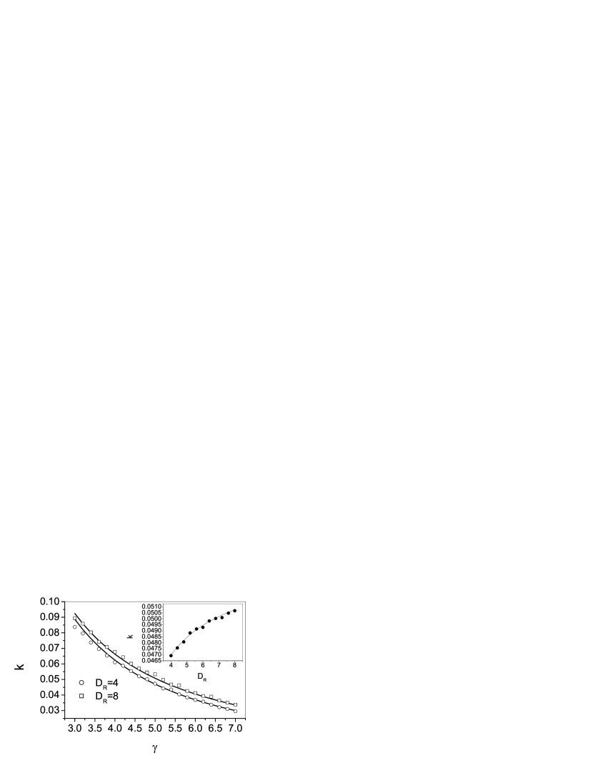
Figure 1: Barrier crossing rate $k$ as a function of dissipation constant $\gamma$ for two different values of effective noise strength $D_{R}$. The solid lines are drawn from theoretical expression, Eq.(49) and the symbols are due to numerical simulation of Eq.(1). The values of the parameters used are $D_{e}=D_{\pi}=2$, $\tau_{e}=\tau_{\pi}=\tau=1$, $\lambda=0$ (open circle) and $\lambda=1$ (open square). Inset: $k$ as a function of $D_{R}$ for $\gamma=5$ and $0\leqslant\lambda\leqslant 1$. Other parameters are same as in the main figure.

IV Numerical Implementation

To judge the potentiality and applicability of our recently developed method for computation of the rate of barrier crossing process, we discuss here both the details of the working equations from the point of view of the numerical implementation and the corresponding simulation of our method. To check the validity and applicability of our model from the point of view of computational implementation, we consider the dynamics in a bistable potential $V(x)=(x^{4}/4)-(x^{2}/2)$ so that the activation energy becomes $E=1/4$. We then numerically solve the Langevin equation (1) by employing stochastic Heun’s algorithm heun1 ; heun2 . The numerical rate has been defined as the inverse of mean first passage time jrc1 ; jrc2 ; mfpt and has been calculated by averaging over 10,000 trajectories. In our simulation we have always used $\tau_{\epsilon}=\tau_{\pi}=\tau=1$ such that the effective correlation time $\tau_{R}$ is always equals to 1, independent of values of the other parameters. To ensure the stability of our simulation, we have used a small integration time step $\Delta t=0.001$ so that $\Delta t/\tau_{R}\ll 1$. To compare our theoretical prediction with numerical simulation we consider the case where the system is solely driven by an external correlated colored noise [see Eq.(49)]. As the degree of correlation between the two noise processes is increased the strength of effective noise strength $D_{R}$ increases (see Eq.(5)). This effectively pumps more energy into the system through which the escape rate should increase. In Fig.(1) we see this effect clearly where the escape rate $k$ is plotted as a function of the dissipation constant $\gamma$ (in the limit of moderate to large friction regime) for two different values of effective noise strength $D_{R}$ which are evaluated by using two extreme values of the degree of correlation $\lambda$ (0 and 1). In the inset we show more explicitly how the system receives more energy through $D_{R}$ as the degree of correlation increases. This behavior suggests that in a properly designed experiment one can enhance the escape rate by externally controlling the degree of correlation between the external fluctuations.

V Conclusions

In this paper, we have generalized the Kramers’ theory of activated rate processes for non-equilibrium open system where the system is driven by two external cross-correlated noise processes with the assumption that the underlying dynamics is non-Markovian. The theory takes into account both the external and internal fluctuations in a unified way. The external fluctuations considered are stationary, Gaussian. Our treatment is valid for intermediate to strong damping limit. We have shown that not only the motion at the barrier top is influenced by the cross correlation between the external fluctuations, it has an important role to play in establishing the stationary state near the bottom of the source well for open system. The stationary distribution function in the well depends significantly on the degree of correlation of the external noise processes. We then derived the generalized Kramers’ rate for the open system and examined several limiting cases. To establish the applicability and potentiality of our recently developed method, we then numerically simulated the dynamics in a model bistable potential and compared with one of the limiting cases. Our results generated via numerical simulation reflect a good agreement with the corresponding values obtained analytically. Our numerical analysis clearly depicts that the escape rate can be enhanced by increasing the degree of correlation between the external fluctuations.

- (1) H. A. Kramers, Physica 7, 284 (1940).
- (2) P. Hänggi, P. Talkner and M. Borkovec, Rev. Mod. Phys. 62, 251 (1990).
- (3) V. I. Mel’nikov, Phys. Rep. 209, 1 (1991).
- (4) E. Pollak and P. Talkner, Chaos 15, 026116 (2005).
- (5) A. Simon and A. Libchaber, Phys. Rev. Lett. 68, 3375 (1992).
- (6) E. W.-G. Diau, J. L. Herek, Z.H. Kim, and A. H. Zewail, Science 279, 847 (1998).
- (7) L. I. McCann, M. I. Dykman, and B. Golding, Nature 402, 785 (1999).
- (8) U. Weiss, Quantum Dissipative Systems (World Scientific, Singapore, 1999).
- (9) A. Nitzan, Chemical Dynamics in Condensed Phases (Oxford University Press, Oxford, 2006).
- (10) R. Kubo, M. Toda, N. Hashitsume, and N. Saito, Statistical Physics II: Nonequilibrium Statistical Mechanics, 2nd edition (Springer, Berlin, 1995).
- (11) R. Zwanzig, J. Stat. Phys. 9, 215 (1973); M. I. Dykman and M. A. Krivoglaz, Phys. Status Solidi B 48, 497 (1971).
- (12) K. Lindenberg and B. J. West, The Nonequilibrium Statistical Mechanics of Open and Closed Systems (VCH Publisher, Inc., New York, 1990).
- (13) W. Horsthemke and R. Lefever, Noise-induced transitions (Springer, Berlin, 1994).
- (14) J. Ray Chaudhuri, S. K. Banik, B. C. Bag, and D. S. Ray, Phys. Rev. E. 63, 061111 (2001).
- (15) S. K. Banik, J. Ray Chaudhuri, and D. S. Ray, J. Chem. Phys. 112, 8330 (2000).
- (16) J. Ray Chaudhuri, D. Barik and S. K. Banik, Phys. Rev. E 73, 051101 (2006); ibid 74, 061119 (2006).
- (17) I. I. Fedchenia, J. Stat. Phys. 52, 1005 (1988).
- (18) A. Fulinski and T. Telejko, Phys. Lett. A 152, 11 (1991).
- (19) A. J. R. Madureira, P. Hänggi, and H. S. Wio, Phys. Lett. A 217, 248 (1994).
- (20) D. Mei, C. Xie, and L. Zhang, Phys. Rev. E 68, 051102 (2003).
- (21) C. J. Tessone, H. S. Wio and P. Hänggi, Phys. Rev. E 62 4623 (2000) and references therein.
- (22) C. Xie, D. Mei, L. Cao, and D. J. Wu, Eur. Phys. J. B 33, 83 (2003); P. Majee and B. C. Bag, J. Phys. A 37, 3353 (2004).
- (23) N. G. van Kampen, Stochastic Processes in Physics and Chemistry (North Holland, Amsterdam, 1992), Sect. IX.5.
- (24) J. Masoliver and J. M. Porrà, Phys. Rev. E 48, 4309 (1993).
- (25) S. A. Adelman, J. Chem. Phys. 64, 1024 (1976).
- (26) The reduced distribution function is defined as .
- (27) R. F. Grote and J. T. Hynes, J. Chem. Phys. 73, 2715 (1980).
- (28) P. Hänggi and F. Mojtabai, Phys. Rev. A 26, 1168 (1982).
- (29) T.C. Gard, in Monographs and Textbooks in Pure and Applied Mathematics (Marcel Dekker, New York, 1987), Vol.114.
- (30) R. Toral, in Computational Field Theory and Pattern Formation, edited by P.L. Garrido and J. Marro, Lecture Notes in Physics, Vol.448 (Springer-Verlag, Berlin, 1995).
- (31) C. Mahanta and T. G. Venkatesh, Phys. Rev. E 58, 4141 (1998); D. Barik, B. C. Bag, and D. S. Ray, J. Chem. Phys. 119, 12973 (2003).