Linear and nonlinear low frequency electrodynamics of the surface superconducting states in an yttrium hexaboride a single crystal

Abstract

We report the low-frequency and tunneling studies of yttrium hexaboride single crystal. Ac susceptibility at frequencies 10 - 1500 Hz has been measured in parallel to the crystal surface DC fields, $H_{0}$. We found that in the DC field $H_{0}>H_{c2}$ DC magnetic moment completely disappears while the ac response exhibited the presence of superconductivity at the surface. Increasing of the DC field from $H_{c2}$ revealed the enlarging of losses with a maximum in the field between $H_{c2}$ and $H_{c3}$. Losses at the maximum were considerably larger than in the mixed and in the normal states. The value of the DC field, where loss peak was observed, depends on the amplitude and frequency of the ac field. Close to $T_{c}$ this peak shifts below $H_{c2}$ which showed the coexistence of surface superconducting states and Abrikosov vortices. We observed a logarithmic frequency dependence of the in-phase component of the susceptibility. Such frequency dispersion of the in-phase component resembles the response of spin-glass systems, but the out-of-phase component also exhibited frequency dispersion that is not a known feature of the classic spin-glass response. Analysis of the experimental data with Kramers-Kronig relations showed the possible existence of the loss peak at very low frequencies ($<5$ Hz). We found that the amplitude of the third harmonic was not a cubic function of the ac amplitude even at considerably weak ac fields. This does not leave any room for treating the nonlinear effects on the basis of perturbation theory. We show that the conception of surface vortices or surface critical currents could not adequately describe the existing experimental data. Consideration of a model of slow relaxing nonequilibrium order parameter permits one to explain the partial shielding and losses of weak ac field for $H_{0}>H_{c2}$.

I Introduction

There is a growing interest in exploring physical properties of materials involving boron-cluster compounds because of a wide variety of applications SER . Due to $sp^{2}$ hybridization of valence electrons, large coordination number and short covalent radius, boron atoms prefer to form strong directional bonds with various elements. A large number of experimental and theoretical studies are concentrated on the families of compact B₁₂ icosahedrons and B₆ octahedrons with a large diversity of electrical and magnetic characteristics. The highest critical temperatures of the transition to the superconducting state in MB₆ and MB₁₂ compounds were found in YB₆ with $T_{c}\leq 8.4$ K and ZrB₁₂ with $T_{c}\approx 6.0$ K FSK . Both materials have a highly symmetrical crystal structure (CaB₆type for YB₆ and UB₁₂ type for ZrB₁₂) that can be described as boron cages in which yttrium or zirconium atoms develop large vibrational amplitudes with an Einstein-like (nearly dispersionless) lattice mode. In spite of some common features, the two crystals have a few distinct physical characteristics: (i) while YB₆ is a classical type-II superconductor SKUN , ZrB₁₂ (at least, for temperatures above 4.5 K) may be regarded as a textbook example of type-I superconductor GLT ; (ii) while the superconducting properties are enhanced at the ZrB₁₂ surface GLT , they are suppressed in a YB₆ surface (see our tunneling data below). Therefore, ZrB₁₂ and YB₆ samples may serve as model systems for investigating surface-related superconducting effects.

Nucleation of a superconducting phase in a thin surface sheath, when the DC magnetic field, $H_{0}$, parallel to the sample surface decreases, was predicted in 1963 by Saint-James and de Gennes in their seminal work PG . They showed that the nucleation occurs for $H_{0}<H_{c3}=2.39\kappa H_{c}$, where $H_{c}$ is the thermodynamic critical field and $\kappa$ is the Ginzburg-Landau(GL) parameter. Experimental measurements confirm this prediction STR ; PAS ; BURG ; ROLL ; SWR ; OST ; HOP , and it was found that at low frequencies a sample in a surface superconducting state (SSS) shows ac losses with a peak whose position with respect to the DC field depends on the ac amplitude. The peak magnitude exceeds the losses observed either in the normal state ($H_{0}>H_{c3}$) or in the bulk superconducting state($H_{0}<H_{c2}$). It was also predicted that the $H_{c3}/H_{c2}$ ratio, is temperature independent. In contrast, a decrease of this ratio was found in the vicinity of $T_{c}$ in several experiments OST ; HOP . This behavior was associated with the distribution of $T_{c}$ at the surface HU .

In the last few years the SSS has attracted renewed interest from various directions TS2 ; JUR ; GM ; SCOL ; LEV2 ; GLT . Stochastic resonance phenomena in Nb single-crystal were observed in the SSS  TS2 . In JUR it was assumed that at $H_{0}\leq H_{c3}$ the sample surface consists of many disconnected superconducting clusters and subsequently the percolation transition takes place at $H_{c3}^{c}=0.81H_{c3}$. The paramagnetic Meissner effect is also related to the SSS  GM . Voltage noise and surface current fluctuations in Nb in the SSS have been investigated  SCOL . SSS’ were found also in single crystals of ZrB₁₂ LEV2 . In agreement with the previous data ROLL it was demonstrated LEV2 that the waveform of the surface current in an ac magnetic field has a non-sinusoidal character. A simple phenomenological relaxation model provides the good explanation of the experimental data for DC fields near $H_{c2}$ only LEV2 . The relaxation rate in this model depends on the ac frequency and decreased with decreasing $\omega$ LEV2 . Detailed experimental study of the linear ac response in the SSS of single crystals Nb and ZrB₁₂ was published recently in our paper GLT . We showed that ac SSS losses in these materials could be considered in the achieved experimental accuracy as a linear ones and for several DC fields the real part of the ac magnetic susceptibility exhibited a logarithmic frequency dependence as for a spin-glass system.

In spite of the extensive studies, the origin of low frequency losses in SSS is not clear as yet. The critical state model developed for the SSS in FINK implies that if the amplitude of the ac field, $h_{0}$, is smaller than some critical value the losses disappear. The authors of Ref. ROLL claimed that the experiment on Pb-2$\%$In alloy confirms this prediction. On the other hand, the observed response JUR for an excitation amplitude of 0.01 Oe that is considerably smaller than used in ROLL showed losses in SSS in Nb sample at a frequency 10 Hz. Our measurement on Nb and ZrB₂ single crystals also have shown that the out-of-phase part of the ac susceptibility, $\chi_{1}^{\prime\prime}$, was finite at low excitation level GLT . We consider these results as an indication of the inadequacy the critical state model for description of the ac response in SSS. If we assume that the reason for this discrepancy with experimental data, is the small value of the critical surface current, which is much smaller than the current amplitudes at the surface, then we have to expect a decreasing of the losses approximately as $1/h_{0}$ when the amplitude of the applied ac field, $h_{0}$, increases. On the contrary, $\chi_{1}^{\prime\prime}$ increases with $h_{0}$. The ac investigation of YB₆ samples has some advantage due to actually ideal type II magnetization curves in this material that permits one to avoid possible difficulties in the interpretation of the experimental data. The experiment showed that near the transition temperatures SSS exist also in the fields below $H_{c2}$. We found that some features of nonlinear response took place at a very weak ac field with amplitude $\simeq 0.005$ Oe. The ac response at the third harmonic of the fundamental frequency did not leave any room for the perturbation theory. It was proposed that the losses in SSS are due to the slow relaxation of the order parameter at the surface and could not be ascribed to surface vortices. We found that for small $h_{0}$ in quasilinear approximation the integral equation with power dependent nuclear governed the time behavior of the magnetization in ac fields. Some features of the ac response resemble the ones of spin-glass system but one has to note that SSS present a different system with its unique properties.

II Experimental Details

II.1 Sample preparation

The yttrium hexaboride single crystal was grown by the inductive floating zone method of a powder sintered rod with an optimal composition YB_6.85 under 1.2 MPa of argon. According to the Y - B phase diagram, composition with the Y:B=1:6 ratio has undergoes peritectic melting MAS and irrespective of the Y/B ratio the YB₄ single crystal with preferential orientation [001] begins to grow. After enrichment of the melting zone by boron (flux method modification) the yttrium hexaboride single crystals with the [100] orientation grow with the composition of YB_5.79±0.02 (ESD). The total impurity concentration is less than 0.001 % in weight and the obtained lattice parameter is 4.1001(4) Å in accordance with published data COM . These single crystals exhibited a sharp superconducting transition with $T_{c}\approx 7.15$ K.

II.2 DC and ac measurements

The magnetization curves were measured using a commercial SQUID magnetometer. In-phase and out-of-phase components of the ac susceptibility at the fundamental frequency, and the response at the third harmonic were measured using the pick-up coil method SH ; ROLL . A home-made setup was adapted to the SQUID magnetometer, and the block diagram of the experimental setup was published in Ref. LEV2 . The crystal ($10\times 3\times 1$ mm³) was inserted into one of a balanced pair of coils. The unbalanced signal and the third harmonic signal as a function of the external parameters such as temperature, DC magnetic field, frequency and amplitude of excitation, were measured by a lock-in amplifier. The experiment was carried out as follows. The sample was cooled down at zero magnetic field (ZFC). Then the DC magnetic field, $H_{0}$, was applied. The amplitudes and the phases at all frequencies of both signals were measured in a given $H_{0}$ (including at zero field). The excitation amplitude,$h_{0}$, was $0.0005\div 0.5$ Oe. It is assumed that in $H_{0}=0$, and at low temperature, the ac susceptibility equals to the DC susceptibility in the Meissner state with negligible losses. This permits us to find the absolute values of the in-phase and out-of-phase components of the ac susceptibility for all applied DC and ac fields and for all frequencies. Both $H_{0}$ and $h_{0}$ were parallel to the longest sample axis.

II.3 Tunneling measurements

Measurements of the tunneling spectra were carried out using a home made scanning tunneling microscope. The YB₆ single crystal was mounted inside the cryogenic scanning tunneling microscope and then cooled down to 4.3 K. The $dI/dV$ vs. $V$ tunneling spectra (proportional to the local density of states) were acquired using a conventional lock-in technique, while momentarily disconnecting the feedback loop.

III Experimental results

III.1 Tunneling characteristics

Direct information about the energy gap value $\Delta_{0}=\Delta(T=0)$ at the surface of YB₆ was obtained from the tunneling spectra. The ratio $2\Delta_{0}/T_{c}$ is a well known indicator of the electron-phonon coupling strength CARB . Two previous tunneling studies of YB₆ were performed on a single-crystal SKUN and on thin films SCHN and the $\Delta_{0}$ obtained were: 1.22 SKUN and 1.24 SCHN which yields the ratio $2\Delta_{0}/T_{c}\approx 4$. In both cases the tunneling contacts were connected to underlying layers, and hence, monitored bulk properties. Therefore those values which signified a nearly strong coupling are attributed to the bulk characteristics. It was confirmed, in particular by Lortz et al. JUNO , who measured the deviation function $D(T)=H_{c}(T)/H_{c}(0)-(1-(T/T_{c})^{2})$ and found that the value of $2\Delta_{0}/T_{c}$ is slightly above 4.0. Our tunneling spectroscopy results were obtained by STM and therefore better reflect the density of states at the surface. In contrast to our previous measurements on ZrB₁₂ single crystals that showed very high spatial homogeneity GLT , the superconductivity in the present case appeared to be degraded on parts of the YB₆ sample surface, where nearly featureless tunneling spectra were observed. In other regions, however, reproducible ratios of differential conductances in superconducting and normal states $(dI/dV)_{s}/(dI/dV)_{n}$ showing very clearly that BCS-like gap structures were acquired, such as presented in Fig. 1 (solid line).

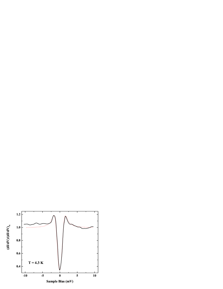
Figure 1: Representative tunneling spectrum of YB₆ at T 4.3 K (solid line) together with its fit to the Dynes function (see text) shown by a dashed line, with fitting parameters $\Delta(T)=1.0$ meV and $\Gamma=0.10$ meV. The spectra were normalized to the normal tunneling conductance at 5 meV (well above the superconducting gap) .

The spectra were compared with a temperature-smeared version of the Dynes formula DYN wich takes into account the effect of incoherent scattering events by introducing a damping parameter $\Gamma$ into the conventional BCS expression for a quasiparticle density of states

$$N_{S}(E)=N_{N}(0)Re[(E-i\Gamma)/\sqrt{(E-i\Gamma)^{2}-\Delta^{2}(T)}].$$ (1)

A very good fit to the experimental data (except for a small asymmetry in the normal resistance between negative and positive bias, the origin of which is not yet clear to us) was achieved with $\Delta(4.3K)=1.0$ meV and $\Gamma=0.10$ meV. Recalling that the experimental spectrum was acquired at $T=4.3$ K, which is about 0.6T_c, with the BCS $\Delta(T)$ dependence TNK we obtain the zero-temperature value $\Delta(T=0)=1.1$ meV. With that, we find that $2\Delta_{0}/T_{c}\approx 3.59$, very close to the BCS weak coupling value of 3.53. In contrast to ZrB${}_{1}2$, we assume that in YB₆ the electron-phonon strength is suppressed at the surface to a weak coupling state.

III.2 DC and ac magnetic characteristics

Fig. 2 demonstrates the temperature dependence of the sample magnetic moment.

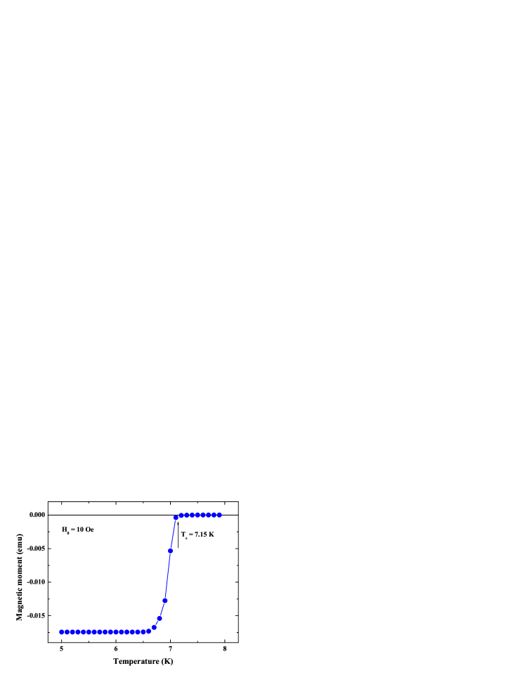
Figure 2: (Color online) Temperature dependence of magnetic moment after ZFC.

In this curve one can see that T${}_{c}\approx 7.15$ K.

From the hysteresis curve measured at 4.5 K, shown in Fig. 3,

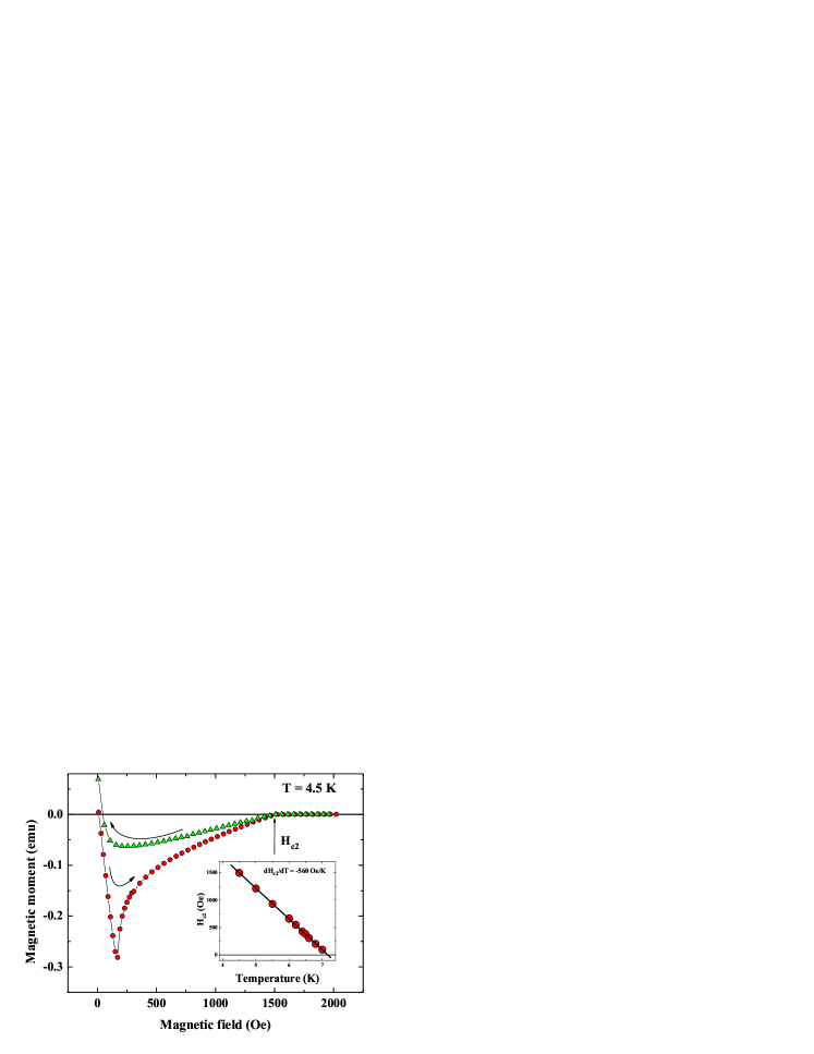
Figure 3: (Color online) Magnetization curve at $T=4.5$ K after ZFC. Inset: temperature dependence of $H_{c2}$.

we are able to evaluate H${}_{c}=295$ Oe, H${}_{c2}=1500$ Oe and GL parameter $\kappa_{1}=H_{c2}/\sqrt{2}H_{c}=3.58$. Using the relation $\frac{dM}{dH_{0}}|_{H_{0}=H_{c2}}=1/4\pi\beta_{A}(2\kappa_{2}^{2}-1)$ one can obtain that $\kappa_{2}=3.3$, where $\beta_{A}=1.16$. The temperature dependence of H_c2 is shown in the inset of Fig. 3. The London penetration depth at T=0, $\lambda_{L}(0)$, can be estimated by using $H_{c2}(T)$ near $T_{c}$, $dH_{c2}/dT\approx-560$ Oe/K, $1/\lambda_{L}(0)=\sqrt{\frac{\pi T_{c}}{\phi_{0}\kappa_{1}^{2}}|\frac{H_{c2}}{dT}|}$ ABR , and $\lambda_{L}(0)\approx 1.4\times 10^{-5}$ cm.

Fourier analysis of the magnetization, $M(t)$, under applied ac and DC fields, $H(t)=H_{0}+h_{0}\cos(\omega t)$, yields an expression: $M(t)=M_{0}(H_{0},h_{0})+\sum_{n}\frac{1}{2}\chi_{n}(H_{0},h_{0})h_{0}\exp(-in\omega t)$. In this paper we discuss the results for $\chi_{1}$ and $\chi_{3}$ susceptibilities. The field dependence of $\chi_{1}(H_{0})$ at $T=4.5$ K and $h_{0}=0.05$ Oe for some frequencies is shown at Fig. 4. One can readily see that the curves shift toward higher DC fields with frequency.

Figure 4: (Color online) Magnetic field dependencies of $\chi_{1}^{{}^{\prime}}$ and $\chi_{1}^{{}^{\prime\prime}}$ at $T=4.5$ K at different frequencies $\omega$.

Decreasing the ac amplitude produces a similar effect. The curves shift to the higher field when $h_{0}\longrightarrow 0$ ( Fig. 5).

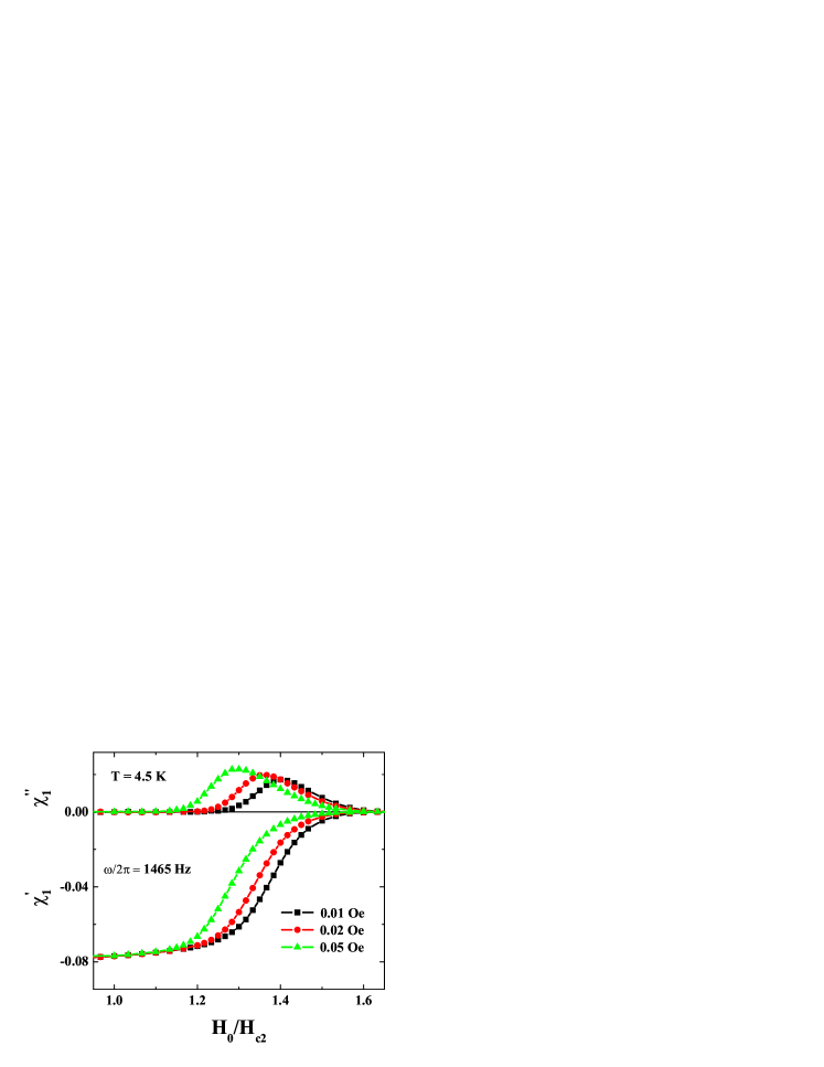
Figure 5: (Color online) Magnetic field dependencies of $\chi_{1}^{{}^{\prime}}$ and $\chi_{1}^{{}^{\prime\prime}}$ at $T=4.5$ K at different amplitudes of excitation, $h_{0}$.

Similar effects were reported for a Pb-2%In sample in Ref. ROLL .

The typical magnetic field dependence of the nonlinear response, $\chi_{3}$, is presented at Fig. 6 for $h_{0}=0.05$ Oe and various frequencies.

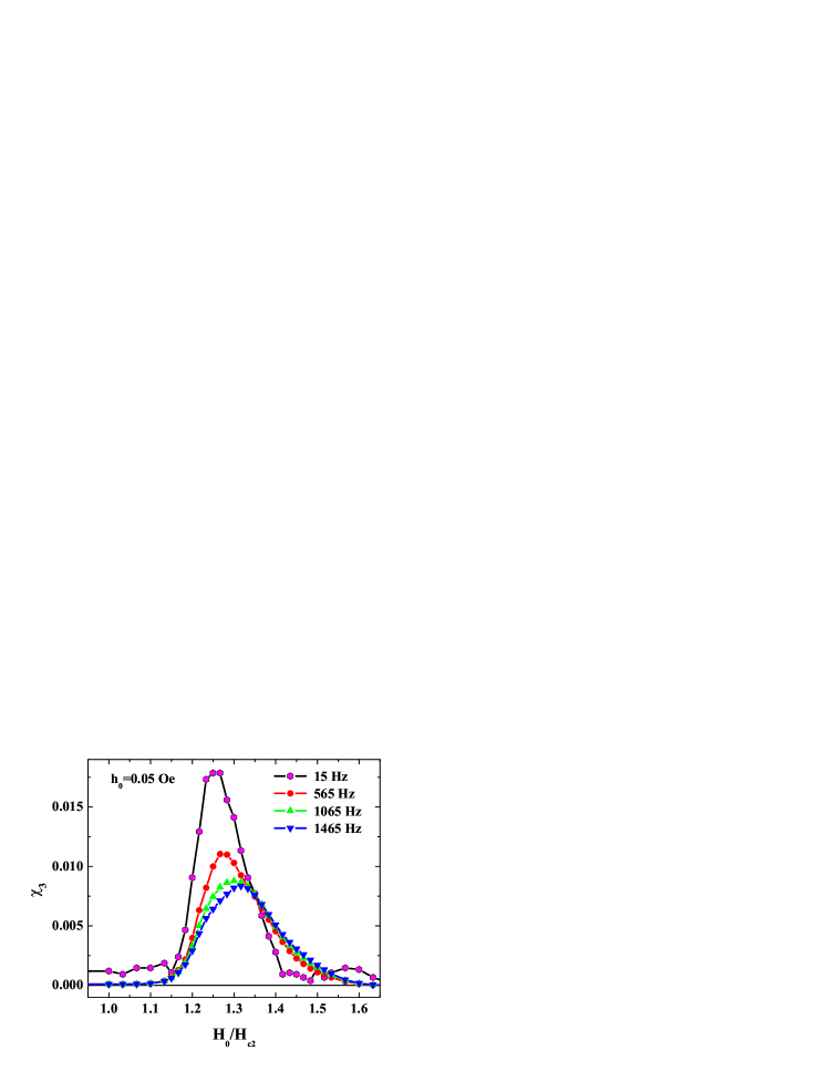
Figure 6: (Color online) Third order susceptibility, $\chi_{3}$, versus reduced magnetic field, $H_{0}/H_{c2}$, at different frequencies.

When the frequency increases the maximum in $\chi_{3}$ moves toward larger DC fields as was observed for $\chi_{1}^{\prime\prime}$ . The frequency dispersion is illustrated on the Cole-Cole plot, Fig. 7.

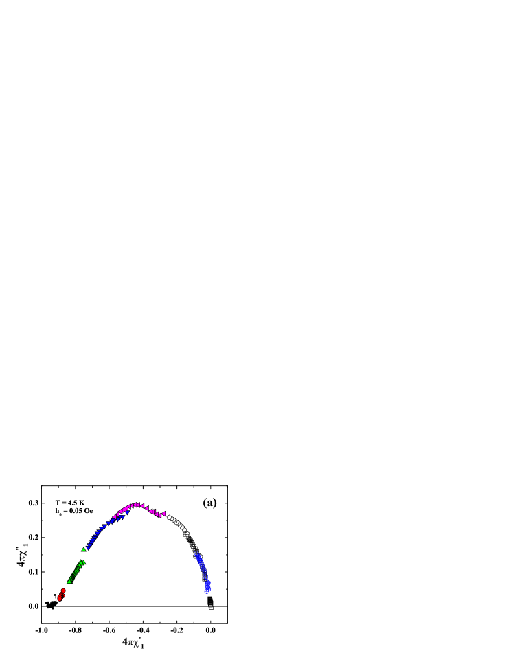
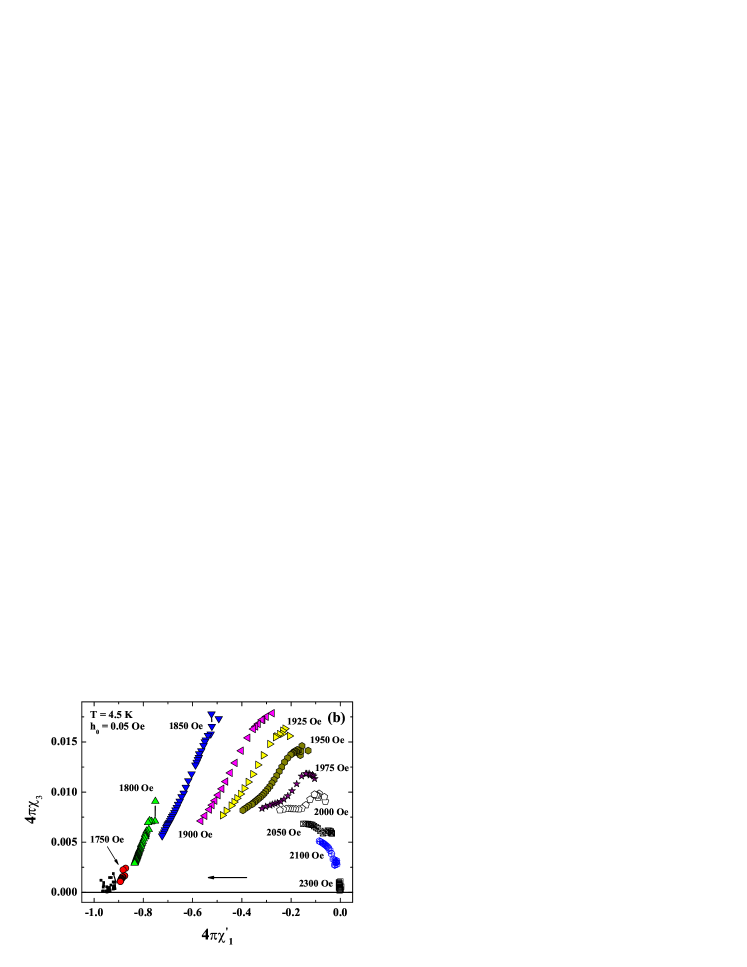
Figure 7: (Color online) Panel (a): Cole-Cole plot of the first harmonic ac susceptibility. Panel (b): $\chi_{3}$ versus $\chi_{1}^{\prime}$. Frequency $\omega$ and DC field $H_{0}$ are parameters for these parametric curves. The symbols on the both panels are the same.

One can see $\chi_{1}^{\prime\prime}$ (panel a) and $\chi_{3}$ (panel b) as a function of $\chi_{1}^{\prime}$ when the frequency increases from 15 to 1465 Hz while the DC field was kept constant. Each disconnected curve of this figure corresponds to different DC fields, the values of which are indicated in panel (b). The arrow in panel (b) shows the direction of increasing frequency along the curves and shielding, as well as $|\chi_{1}^{\prime}|$. Below $H_{c2}$ $4\pi\chi_{1}^{\prime}=-1$ (see Fig. 4). For $H_{0}>H_{c2}$ both $\chi_{1}^{\prime\prime}$ and $\chi_{3}$ decrease as the frequency increases while for $H_{0}$ close to $H_{c3}$ they increase.

Fig. 8 shows the field dependence of $\chi_{3}$ at $\omega/2\pi=1465$ Hz and various amplitudes of excitation, $h_{0}$.

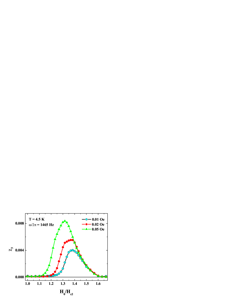
Figure 8: (Color online) Third order susceptibility, $\chi_{3}$, versus reduced magnetic field, $H_{0}/H_{c2}$, at different amplitude of excitation.

The third harmonic cannot be adequately described in the frame of the perturbation theory which predicts that $\chi_{3}\propto h_{0}^{2}$. For example, at $H_{0}/H_{c2}=1.3$, $\chi_{3}$ depends on $h_{0}$ strongly, while at $H_{0}/H_{c2}=1.45$, $\chi_{3}$ is almost constant (see Fig. 8). We can discuss only the dependence of $\chi_{3m}$ (defined as the maximum value of the $\chi_{3}(H_{0})$ curve for any given frequency) on the ac amplitude $h_{0}$. Fig. 9 demonstrates that $\chi_{3m}\approx h_{0}^{0.2}$ in contrast to what the perturbation theory predictions.

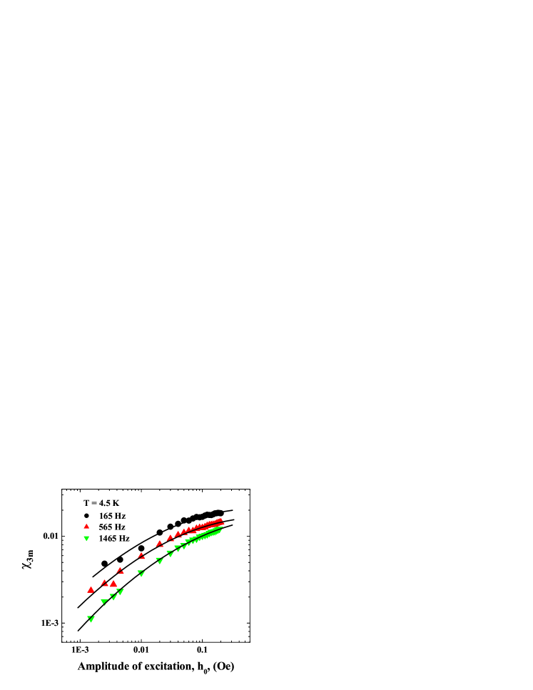
Figure 9: (Color online) Amplitude dependence of the third order susceptibility at maximum, $\chi_{3m}$, at different frequencies (see text).

Below we consider the experimental results obtained at higher temperatures. Fig. 10 demonstrates the field dependence of $\chi_{1}$ at frequency $\omega/2\pi=1065$ Hz and $h_{0}=0.05$ Oe at various temperatures.

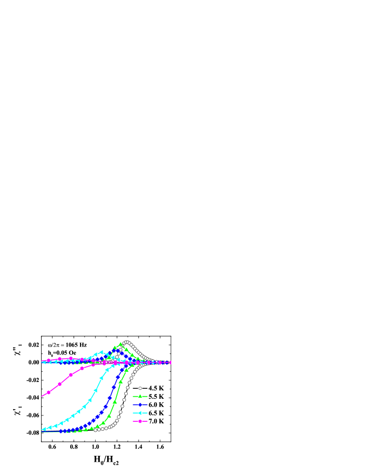
Figure 10: (Color online) Field dependence of $\chi_{1}^{\prime}$ and $\chi_{1}^{\prime\prime}$ for various temperatures.

The peak in $\chi_{1}^{\prime\prime}$ shifts toward $H_{c2}$ with temperature and at 7 K this peak is located already below $H_{c2}$. One can see in the Fig. 10 that for $T<7$ K full shielding ($\chi_{1}^{\prime}=-1/4\pi$) is observed at low $H_{0}$, whereas at 7 K only partial shielding is observed at low DC field. Also Fig. 11 shows that in the vicinity of $T_{c}$ $\chi_{3m}$ lies below $H_{c2}$. Because we did not observed any absorption peak and harmonic signal in the mixed state we consider that SSS are responsible for the experimental observations at $T=7$ K too. Existence of the SSS below $H_{c2}$ was predicted by H. Fink in 1965 HF .

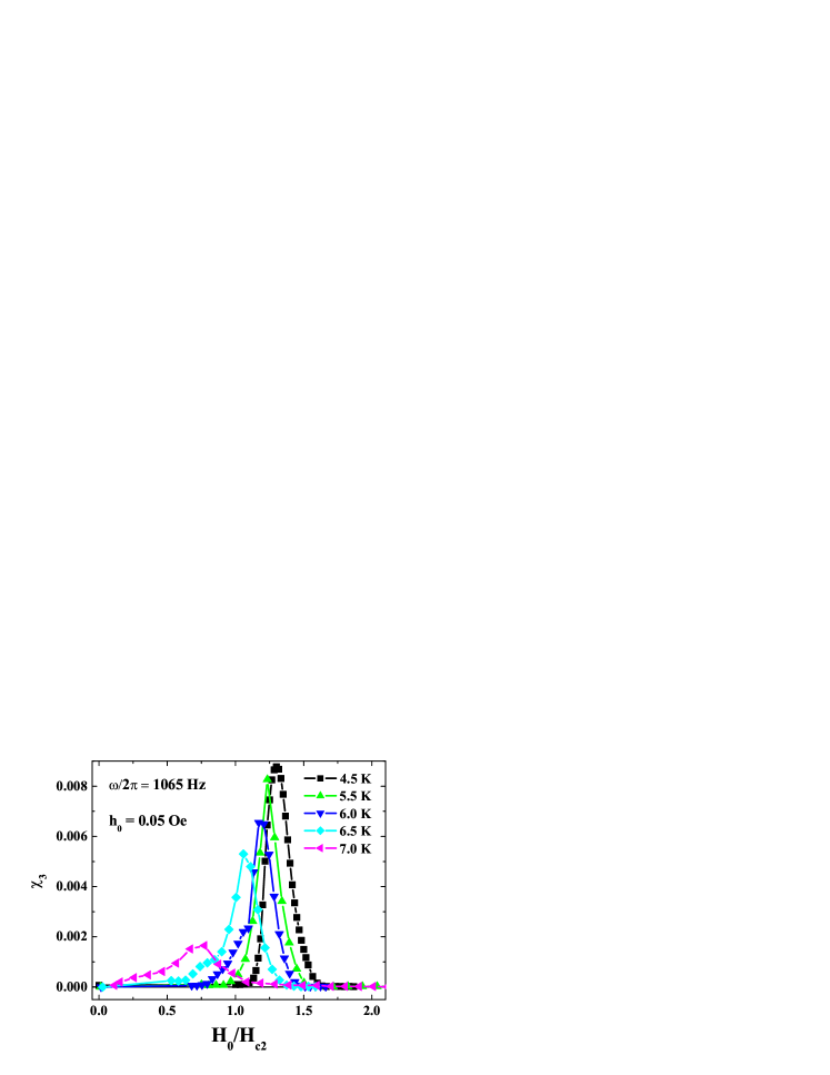
Figure 11: (Color online) Field dependence of $\chi_{3}$ for different temperatures.

Increasing the DC field we can reach the field at which $\chi_{1}$ or $\chi_{3}$ becomes zero. This field can be considered as the third critical magnetic field $H_{c3}$. Both conditions actually give the same value of $H_{c3}$. The experiment shows that the $H_{c3}/H_{c2}$ ratio decreases with temperature.

IV Theoretical model

Let us consider a superconducting slab of thickness 2$L$ in the parallel to its surface external DC and ac magnetic fields. Due to the considerably short relaxation time of the order parameter TNK ; TR one can use the stationary GL equations. We choose the coordinate system in which the $x$-axis is perpendicular to the slab surface, the plane $x=0$ is in the center of the slab, and the external magnetic field is directed along the $z$-axis. Looking at the dimensionless order parameter in the form $\Psi(x,y,t)=\phi(x,t)\exp(iky)$ the GL equation can be written as:

$$\ln(T_{c}/T)\{-\phi+|\phi|^{2}\phi\}-\frac{d^{2}\phi}{dx^{2}}+(a-k)^{2}\phi=0,Eq2$$ (2)

$$\frac{d^{2}a}{dx^{2}}=\frac{\ln(T_{c}/T)}{\kappa^{2}}|\phi|^{2}(a-k).$$ (3)

Here $a$ is a $y$-component of the dimensionless vector potential. The order parameter is normalized with respect to the absolute value of the order parameter in zero field, the distances with respect to the coherence length at zero temperature, $\xi_{0}$, ($x\longrightarrow x/\xi_{0},~{}y\longrightarrow y/\xi_{0},~{}l=L/\xi_{0}$) and the vector potential with respect to $\hbar c/2e\xi_{0}$ ($a=A/(\hbar c/2e\xi_{0}$)). The boundary conditions for calculation of surface states are $\phi(0,t)=d\phi(\pm l,t)/dx=0$ and $a(0,t)=0,~{}da(\pm l,t)/dx=\mathfrak{h}(t)$, where $\mathfrak{h}(t)$ is the dimensionless applied magnetic field.

These nonlinear equations can be solved by numerical methods. We add the time derivative $\partial\phi/\partial t$ into the right side of Eq. (2) and seek the stationary solutions of the Eqs. (2, 3). Replacing the space derivatives by finite differences on the grid with step $dx=l/N$ Eq. (2) transforms into $N$ first order differential equations. The solution of the obtained linear algebraic system can be found by regular method. The grid with N=1000 points was used. In the surface state the order parameter differs from zero only near the surface, at a scale of several coherence lengths, $\xi(T)$. Actually, the choice $L=5\xi(T)\equiv D$ provides good accuracy for calculating $\phi$. The real dimensions of the investigated samples, $L$, considerably exceed this scale by 3-5 orders of magnitude. Parameter $k$ is not a gauge invariant quantity and we choose it using conditions $a=0$ at $x=0$. In SSS the magnetic field in the bulk is constant. So we can obtain $k$ for a thick slab with $L\gg 5\xi(T)$ from the solution of the problem for a thin slab with $D\geq 5\xi(T)$ by gauge transformation

$$k=k_{s}+\mathfrak{h}_{zs}\times(l-d)$$ (4)

and vector potential in the surface layer

$$a(l-d+x)=a_{s}(x)+\mathfrak{h}_{zs}\times(l-d).$$ (5)

Here $d\equiv D/\xi_{0}$, index $s$ corresponds to the problem for a thin slab, and $\mathfrak{h}_{zs}$ is the $z$-component of magnetic field in the center of the thin slab. This note is important for numerical calculations.

V Discussion

It is well known (see, for example, LEV2 ) that for a given external magnetic field there is a whole band of $k$ for which surface solutions exist. These solutions describe the nonequilibrium states and only one solution corresponds to the equilibrium state, for which the magnetic field inside the bulk equals its external value and the total surface current, $J_{s}$, equals zero. Parameter $k$ is an integral constant of the nonstationary GL equations. That is, $k$ is time independent, in contrast to $\phi$, in the frame of the GL model. The relaxation time of the order parameter $\phi$ is considerably shorter than any ac period in our experiment. So when the external magnetic field is changing during the ac cycle, one may expect that $\phi$ follows the instantaneous value of the magnetic field and $k$ remains approximately constant. Let assume that starting from an equilibrium state in some DC field, $H_{0}$, we increase the external magnetic field but simultaneously hold $k$ constant. In this case the surface current $J_{s}$ becomes different from zero. It is possible to consider two definitions of the surface critical current $J_{s1}$ and $J_{s2}$ FINK ; PARK . The first definition of such a critical current is $J_{s1}=(c/4\pi)dh_{s1}$, where $dh_{s1}=H_{1}-H_{0}$ and $H_{1}$ is the field for which the energy of the surface superconducting state equals the energy of the normal state FINK . The second definition is $J_{s2}=(c/4\pi)dh_{s2}$, where $dh_{s2}=H_{2}-H_{0}$ and $H_{2}$ is the field for which SSS disappears. The quantities $dh_{s1}$ and $dh_{s2}$ have different values and different dependencies on the thickness of the sample, $L$. While $dh_{s1}$ dramatically depends on $L$, $dh_{s2}$ for $L>1000\xi$ actually does not. The value of $dh_{s2}$ is considerably larger than $dh_{s1}$ for large $L$. This difference is due to the large contribution of the magnetic field to the system energy, if the magnetic field in the bulk differs from the external field. These features are shown in Figs. 12a, 12b, where $dh_{s1}$ and $dh_{s2}$ are presented as a function of the DC magnetic field for different $L$’s at $T/T_{c}=0.9$.

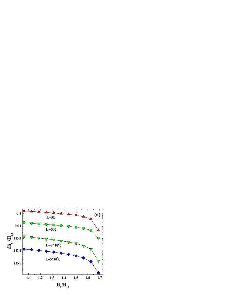
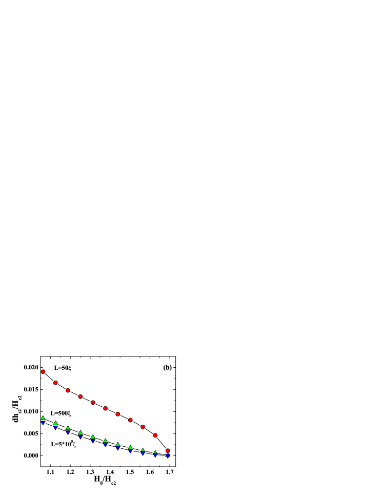
Figure 12: (Color online) Field dependence of the surface critical magnetic field (a) - $dh_{s1}(H_{0}/H_{c2})$ and (b) - $dh_{s2}(H_{0}/H_{c2})$ for different slab thickness, $L$, at $T/T_{c}=0.9$ (see text).

In the reduced variables $dh_{s1}/H_{c2}$ , $dh_{s2}/H_{c2}$, $H_{0}/H_{c2}$ the curves form is actually temperature independent. The assumption of slow relaxing $k$, permits one to understand qualitatively the effect of complete screening of a weak ac field with amplitude $h_{0}\ll H_{0}$ in SSS. Ac surface current $J_{s}(k,H)$ is a function of the instantaneous values of the external magnetic field and $k$. This function can be calculated for a thin slab of several coherence length thickness and then using the gauge transformation, Eqs.(4 and 5), to get a solution for a thick slab. As a function of $k_{s}$ and $H$, the $J_{s}(k_{s},H)$ is a slow function of $H$. For example, at $T=0.9T_{c}$ numerical calculation gives $\frac{\partial h_{zs}(k_{s},H)}{\partial H}=0.88+0.19(H_{zs}/H_{c2}-1)$. Where $H_{zs}$ is magnetic field in the center of the slab. So for a thin slab, an almost complete penetration of the ac field inside the bulk takes place and the value of the surface current is very small. For a thick slab $k\neq k_{s}$ and the requirement of constant $k$ during the ac cycle, implicitly means that $k_{s}$ also changed according to Eqs. (4 and 5). This leads to considerably large surface currents and to screening of the ac field. In reality, we have large dimensionless parameter $L/\xi(T)$ that increases ac field screening. Fig. 13 demonstrates the calculated (in the assumption of constant $k$) $\chi^{\prime}=\Delta M/dh_{s1}$, as a function of the DC field when the external field was increased by $dh_{s1}$.

Figure 13: (Color online) Field dependence of $\chi^{\prime}$ for different slab thickness, $L$, at $T/T_{c}=0.9$ (see text).

It is evident that for any macroscopically large sample, $L\geq 5000\xi$, the complete screening, $\chi^{\prime}=-1/4\pi$, should be obtained for DC fields excluding fields close to $H_{c3}$. However our experiments (Fig. 4) do not confirm this conclusion. We see that $\chi_{1}^{\prime}$ in the field $H_{0}\approx(H_{c2}+H_{c3})/2$ already differs from $-1/4\pi$. It means that slow relaxation of $k$ takes place which leads to the losses and incomplete screening.

For a given ac amplitude, $\chi_{1}^{\prime\prime}$ has a maximum at some values of the DC field defined as $H_{m}$ (see Fig. 5). $H_{m}$ was considered in Ref. BERT as the DC field at which the amplitude of the ac surface current $J_{0s}=(c/4\pi)h_{0}$ equals approximately to the critical value $J_{s1}$. In order to test this in Fig. 14 we show $J_{0s}$ as a function of $H_{0}$ and calculate a critical current $J_{s1}$ for a slab of thickness $L=5\times 10^{5}\xi$. Theoretical data of the $J_{s1}$ were arbitrarily normalized in order obtain the intersection with the experimental curve at $H_{0}/H_{c2}=1.25$. While the theoretical dependence of $J_{s1}$ is almost a linear function of $H_{0}$, the experimental curve starts from $H_{0}/H_{c2}=1.45$ and is a nonlinear function of $H_{0}$.

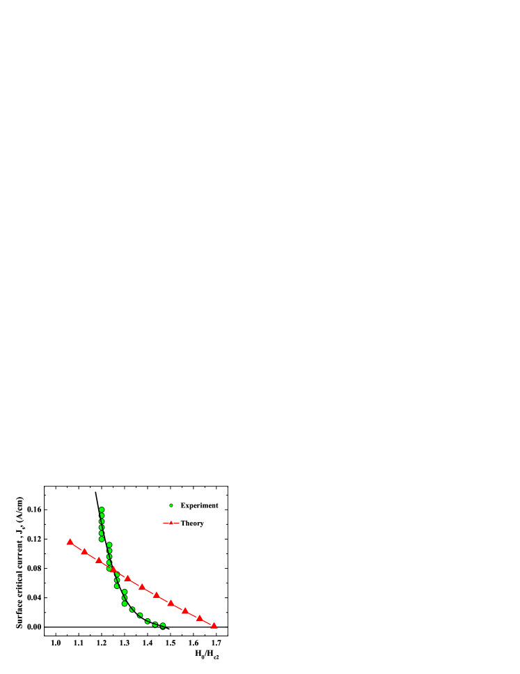
Figure 14: (Color online) Surface critical current $J_{s}$, found with assumption of Ref. BERT , experimental values and calculated $J_{s1}$ as a function of reduced DC field $H_{0}/H_{c2}$ (see text).

One can conclude that losses observed in our experiment are not connected to the condition $h_{0}\approx dh_{s1}$ for $H_{0}>H_{c2}$.

The maximal losses, $\chi_{m}^{\prime\prime}$, at $H_{m}$, as a function of $h_{0}$ is shown at Fig. 15. Inset to Fig. 15 shows that in the limit $h_{0}\rightarrow 0$ the losses do not disappear. In a linear system $\chi_{1}^{\prime\prime}$ should be amplitude independent. While our experiments show a linear dependence $\chi_{m}^{\prime\prime}$ on the ac amplitude (Fig. 15). It does not permit us to consider the response as a linear one even at very low amplitudes of excitation. Therefore more experimental measurements at low ac fields are needed.

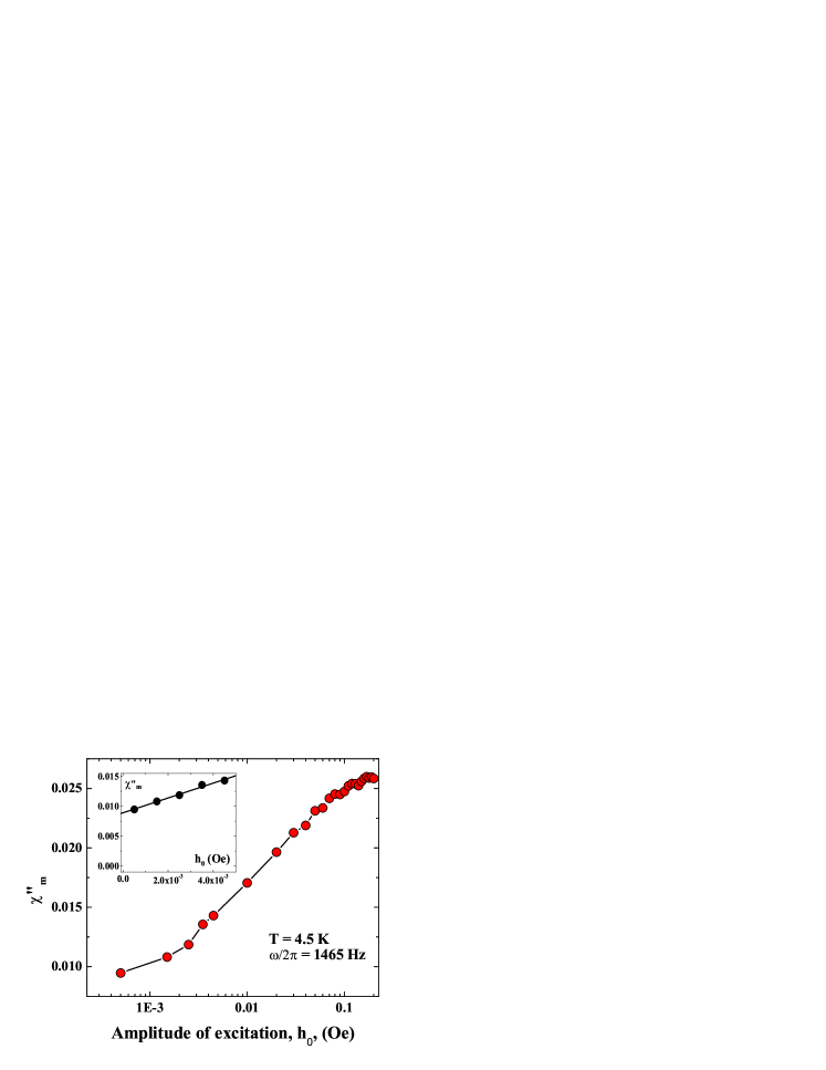
Figure 15: (Color online) Out-of-phase susceptibility at maximum, $\chi_{m}^{\prime\prime}$, as function of an excitation amplitude,$h_{0}$. Inset shows the expanded view for weak $h_{0}$ in linear scale.

In general, the magnetic moment can be presented by following expression:

$$M(t)=\int_{-\infty}^{t}K(t-t^{\prime},h(t^{\prime}))h(t^{\prime})dt^{\prime}.$$ (6)

For $h_{0}\simeq 0.02$ Oe the susceptibilities at higher harmonics are small and we can rewrite Eq. (6) as

$$M(t)=\int_{-\infty}^{t}K(t-t^{\prime},h_{0})h(t^{\prime})dt^{\prime}$$ (7)

considering only the response at the fundamental frequency. Under this approximation, the response at fundamental frequency, matches the Kramers-Kronig relations (KKR):

$$\chi_{1}^{\prime}=\chi_{\infty}+\int_{0}^{\infty}\frac{2\zeta\chi_{1}^{\prime\prime}(\zeta)}{\pi(\zeta^{2}-\omega^{2})}d\zeta$$ (8)

and then

$$\begin{array}[]{c}I(\omega)\equiv\chi_{1}^{\prime}(\omega)-\int_{\omega_{0}}^{\omega_{m}}\frac{2\zeta\chi_{1}^{\prime\prime}(\zeta)}{\pi(\zeta^{2}-\omega^{2})}d\zeta=\\ \chi^{\prime\prime}(\varpi)\int_{0}^{\omega_{0}}\frac{2\zeta d\zeta}{\pi(\zeta^{2}-\omega^{2})}+\chi_{\infty}+\\ \sum_{n}\int_{\omega_{m}}^{\infty}\frac{2\omega^{2n}\chi_{1}^{\prime\prime}(\zeta)}{\pi\zeta^{2n+1}}d\zeta,\end{array}$$ (9)

where $\omega_{0}$ and $\omega_{m}$ are the minimal and maximal available frequencies in our experiment, respectively, and $0<\varpi<\omega_{0}$. $I(\omega)$ can be calculated from the available experimental data and be presented in the form

$$I(\omega)=a+b\ln|1-\omega_{0}^{2}/\omega^{2}|+\sum_{n=1}^{n_{max}}c_{n}\omega^{2n}.$$ (10)

With $c_{n}>0$ we obtain $\chi_{1}^{\prime\prime}(\varpi)=\pi b$. Coefficients $a,~{}b$ and $c_{n}$ could be found by least square fit. For $\omega^{2}/\omega_{m}^{2}<<1$ it is sufficient to take into account only a few terms in Eq. (10). Results of this approach are presented at Fig. 16, where $\chi_{1}^{\prime\prime}(\varpi)$ and $a$ as a function of the DC field are shown.

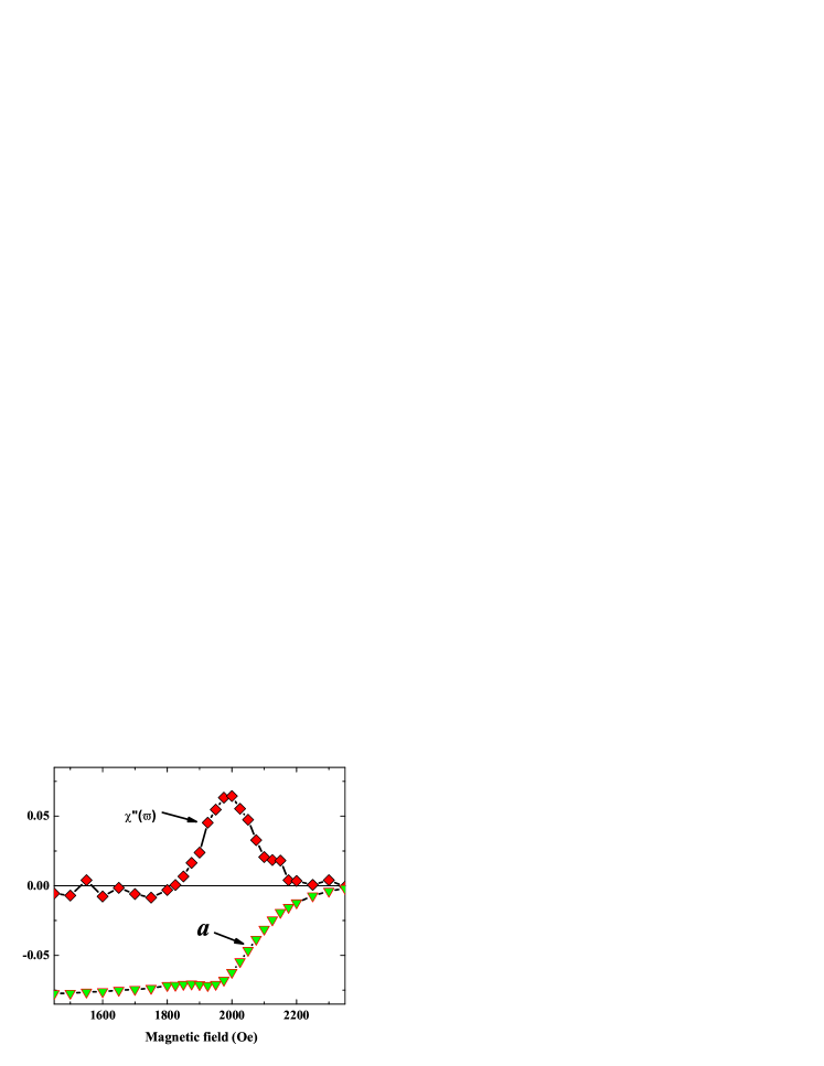
Figure 16: (Color online) Field dependencies of $\chi^{\prime\prime}(\varpi)$ and parameter $a$ of Eq. (10) at $T=4.5$ K and $h_{0}=0.02$ Oe (see text).

The measured data in the frequency range 15-1460 Hz $\chi_{1}$ at $T=4.5$ K, was used for the calculation of $I(\omega)$ for $25<\omega/2\pi<200$ Hz with $\omega_{0}/2\pi=17.5$ Hz and $\omega_{m}/2\pi=1455$ Hz. The approximation of $I(\omega)$ by using expression Eq.(10) with $n_{max}=1$ produces $\chi_{1}^{\prime\prime}(\varpi)$ curve shown in Fig. 16. Because $c_{n}\approx\omega^{2}c_{n-1}/\omega_{m}$ with $\omega^{2}/\omega_{m}^{2}\approx 0.02$ one could expect that expression (7) with $n_{max}=1$ gives the correct result. Taking into consideration the term $c_{2}$ gives unphysical result, because $c_{2}$ is very small and negative. It is due to the scattering of the experimental data and ignores in Eq. (10) the dependence of $\varpi$ on $\omega$. Fig. 16 shows that the calculated loss peak is approximately 3 times larger than the measured losses at $\omega/2\pi>20$ Hz, Fig. 4. Qualitatively this behavior can be explained as follows. Because $\chi_{1}^{\prime\prime}$ exhibits a weak frequency dispersion we can estimate integral in the left side of Eq. (9) by

$$\begin{array}[]{c}R=\int_{\omega_{0}}^{\omega_{m}}\frac{2\zeta\chi_{1}^{\prime\prime}(\zeta)}{\pi(\zeta^{2}-\omega^{2})}d\zeta\\ \cong\chi_{1}^{\prime\prime}(\omega_{m}+\omega_{0}/2)\ln(\frac{\omega_{m}^{2}-\omega^{2}}{\omega_{0}^{2}-\omega^{2}})/\pi.\end{array}$$ (11)

In Fig. 17 we showed the correspondence between the estimated $R$ by Eq. (11) and the result of the numerical calculation of the integral in Eq. (11) at $H_{0}=2000$ Oe).

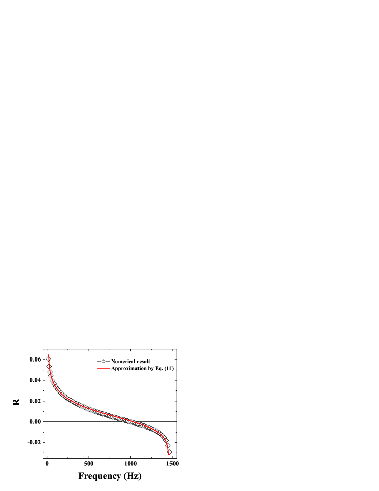
Figure 17: (Color online) Frequency dependence of $R$, numerical calculation and approximation by Eq. (11) (see text).

It is important that $R$ has a positive sign for $\omega/2\pi<1000$ Hz and in the left side of Eq. (9) one has the sum of two negative values. So we should expect a large contribution into the integral in Eq. (8) from frequencies outside the ($\omega_{0},~{}\omega_{m}$) region and the presentation of this contribution in the form of Eq. (9) gives a large value for the term $b$ in Eq. (10).

We believe that the observed in SSS losses are the result of the relaxation $k$ to its equilibrium value. This model can ascribe both the partial screening and losses for $H_{0}>H_{c2}$. The other model assumes that the motion of the of 2D-vortices in the surface sheath KUL is responsible for the losses KAR . These vortices with surface density $n_{s}=H_{0}\sin(\theta)/\phi_{0}$ appear if the applied field has a normal component to the sample surface $H_{n}=H_{0}\sin(\theta)$, due to misalignment, or alternatively if the surface is not sufficiently smooth. One can estimate the conductivity of the surface layer $\sigma=\sigma_{n}H_{c2}/H_{0}\sin(\theta)$ where $\sigma_{n}$ is the conductivity in the normal state. In our sample, $\sigma_{n}\approx 10^{17}$ CGS and the skin depth in the surface layer at frequency $\omega/2\pi=10$ Hz is considerably larger for any real angle( $\simeq 10^{-2}$ rad) to provide sufficient screening of the ac field by a layer with thickness $10^{-5}\div 10^{-6}$ cm.

The ac response of SSS resembles that of the spin-glass systems. Real and imaginary parts of $\chi_{1}$ can be well represented by a polynomial of $\ln(\omega)$ shown in Fig. 18 for $H_{0}=2$ kOe and T=4.5 K.

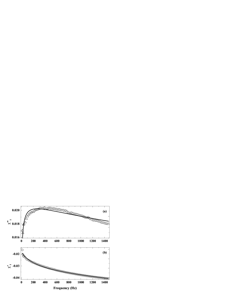
Figure 18: Frequency dependence of $\chi_{1}^{\prime\prime}(\omega)$ (panel (a)) and $\chi_{1}^{\prime}(\omega)$ (panel (b)) for $H_{0}=2$ kOe ($H_{0}=1.25H_{c2}$ )at 4.5 K. Continuous lines present the fit to the second order polynomial of $\ln(\omega)$ (Eq.(11)).

In this figure, presentation of $\chi_{1}\prime$ and $\chi_{1}\prime\prime$ by polynomial

$$a_{0}+a_{1}\ln(\omega)+a_{2}\ln^{2}(\omega)$$ (12)

are shown for a considerably wide frequency region $15<\omega/2\pi<1465$ Hz. For some DC fields the coefficient $a_{2}$ is small and one can get the spin-glass like $\chi_{1}^{\prime}$. But $\chi_{1}^{\prime\prime}$ also exhibits the frequency dispersion that is not typical for spin-glass systems. The ”$\pi/2$” rule IMRY , $\chi_{1}^{\prime\prime}=-\frac{\pi}{2}\frac{d\chi_{1}^{\prime}(\omega)}{d\ln(\omega)}$, is not fulfilled in our data, Fig 19.

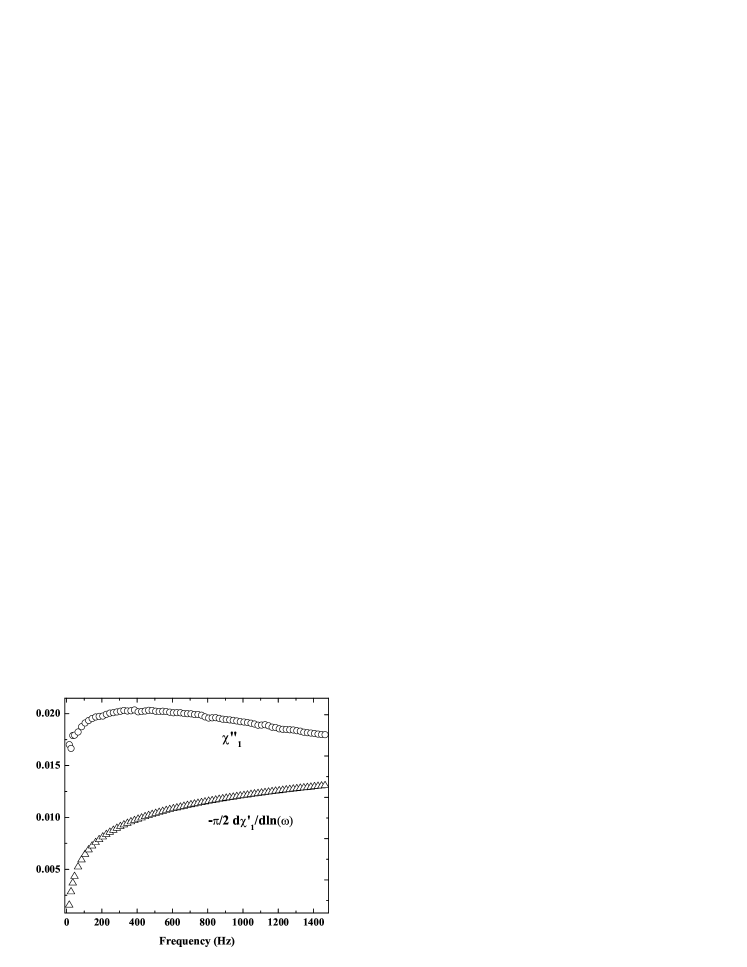
Figure 19: (Color online) The test of the ”$\pi/2$” rule for the experimental data at $T=4.5$ K and $H_{0}=2$ kOe.

The simple relaxation models of ac response is applicable only for a DC field near $H_{c2}$ LEV2 . If in analogy with a spin-glass system we assume that the magnetization moment of the sample, $M(t)$, can be found from the relaxation equation:

$$dM/dt=-\nu M-dh/dt,$$ (13)

with subsequent averaging over the relaxation rates, then

$$\chi_{1}=\int_{0}^{\infty}\widetilde{P}(\nu)\frac{i\omega}{\nu-i\omega}d\nu,$$ (14)

where $\widetilde{P}(\nu)$ is the distribution function of the relaxation rates. Using $1/(\nu-i\omega)=\int_{0}^{\infty}\exp(-(\nu-i\omega)t)\text{dt}$ we transform Eq.(14) to

$$i\chi_{1}(\omega)/\omega=\int_{0}^{\infty}P(\nu)\exp(-\nu t)d\nu,$$ (15)

where $P(t)=\int_{0}^{\infty}\widetilde{P}(\nu)\exp(-\nu t)d\nu$. So, if Eq.(14) describes adequately the experimental data with some $P(\nu)$, then these two integrals should be equal each other

$$\begin{array}[]{c}P(t)=2\int_{0}^{\infty}\chi_{1}^{\prime\prime}(\omega)\cos(\omega t)d\omega/\pi\omega=\\ -2\int_{0}^{\infty}\chi_{1}^{\prime}(\omega)\sin(\omega t)d\omega/\pi\omega.\end{array}$$ (16)

Experimental data are available only for a finite frequency region 15 Hz $<\omega/2\pi<$ 1465 Hz, while integrals in Eq.(16) are expanded for all frequencies and we have to extrapolate our data to the entire frequency axis. This was done assuming that for $\omega/2\pi<15$ Hz and $\omega/2\pi>1465$ Hz $\chi_{1}{\prime\prime}$ is a power function of frequency $\omega^{p}$. As a result, the sin- and cos-Fourier transformations in Eq.(16) give different values for $\widetilde{P}(t)$ as shown at Fig. 20 where the ac response in $H_{0}=1.25H_{c2}$ was used.

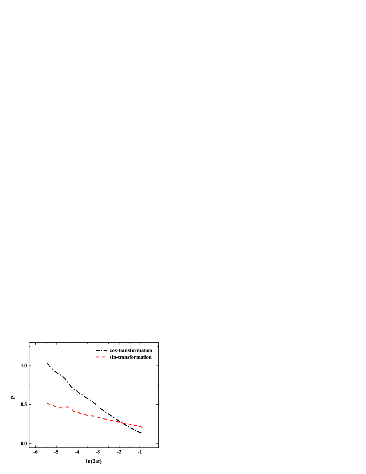
Figure 20: The test of the Eq. (16) on the experimental data at $T=4.5$ K and $H_{0}=2$ kOe.

It is readily seen that the experimental data exclude the possibility consider the SSS as an analog of a spin-glass system. Equation (7) shows that in the quasilinear approximation the magnetization of the samples satisfied an integral equation

$$\int_{-\infty}^{t}G(t-t^{\prime},h_{0})M(t^{\prime})dt^{\prime}=h(t).$$ (17)

It is interesting to notice that the nuclear $G(t,h_{0})$ can be extracted by the Fourier transformation of $1/\chi_{1}(\omega)$. Performing the same procedure as above, we obtained that sin- and cos-Fourier transformations in Eq.(11) yield different values for $G(t,h_{0})$ which is certainly due to the lack of experimental data for whole frequency axis. The extrapolation of the imaginary part of $1/\chi_{1}(\omega)$ gives more accurate results and we consider only the $G(t,h_{0})$ that is obtained by the sin-Fourier transformation of $1/\chi_{1}^{\prime\prime}(\omega)$. Good approximation of $G(t,h_{0})$ provides the expression $G(t,h_{0})=A(t)/t^{q}$ with slow function $A(t)$ for $t>\pi/1465=t_{c}$. For $t<t_{c}$ function $G(t,h_{0})$ is singular, but integral $\int_{0}^{t_{c}}G(t,h_{0})\text{dt}$ has a finite value. The parameters $q$ and $A(t)$, depend on the DC field. For example, in field $H_{0}=1.25H_{c2}$ $q=0.876$ and $A(t)=-\exp(1.285-0.00842\ln^{2}(2\pi t))$. In Fig. 21 we show $G(t,h_{0})$ for some values of the DC magnetic field and the inset presents $q$ versus $H_{0}$.

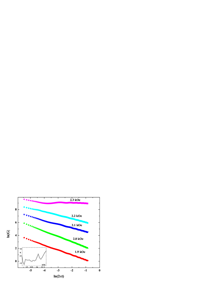
Figure 21: Time dependence of nuclear of Eq. (17) for several DC fields near the absorption maximum at $T=4.5$ K.

So, the dynamics of SSS is governed by an integral equation with retardation. This feature distinguishes SSS from other known systems.

VI Conclusion

In this paper we have studied the low frequency linear and nonlinear dynamics of the SSS of a single crystal of yttrium hexaboride. The tunneling spectra were studied as well. Tunnel measurements allow us to make the assumption, that in this single crystal, unlike ZrB₁₂, near the surface the electron-phonon interaction is suppressed and the situation of weak coupling is realized. We showed that the surface superconducting states define the peculiarities of the low frequency response. In spite of different behavior under magnetic fields (ZrB₁₂ is a type-I superconductor and YB₆ is that of type-II) and different surface properties the two materials exhibit very similar and universal ac characteristics reflecting the nature of the SSS. In both cases we observed a nonlinear response for very weak ac amplitudes (in experiments with YB₆ $h_{0}$ was as small as 0.005  Oe) and the question about the existence of a linear response is open. An extrapolation of the low-amplitude data did not reveal a linear regime. Similar to spin-glass systems (where finite losses at considerably low frequencies exist), the real part of the susceptibility exhibits a logarithmic frequency dependence at some DC magnetic field. But the out-of-phase component has a frequency dispersion. The frequency dispersion in SSS is different from that of the spin-glass systems. The slow relaxation of the phase of an order parameter leads to a frequency dispersion of the ac susceptibility. The analysis of the experimental data by means of Kramers-Kronig relations allow us to make the assumption of the presence of the loss peak at frequencies below 5 Hz.

- (1) T.I. Serebryakova and P. D. Neronov, High-Temperature Borides (Cambridge International Science, Cambridge, 2003).
- (2) Z. Fisk, P.H. Schmidt, and L.D. Longinotti, Mater. Res. Bull. 11, 1019 (1976).
- (3) S. Kunii, T. Kasuya, K. Kadowaki, M. Date, and S.B. Woods. Solid State Commun., 52, 659 (1984).
- (4) M.I. Tsindlekht, G.I. Leviev, V.M. Genkin, I. Felner, Yu. B. Paderno, and V.B. Filippov, Phys. Rev. B 73, 104507 (2006).
- (5) D. Saint-James and P.G. Gennes, Phys. Lett. 7, 306 (1963).
- (6) M. Strongin, A. Paskin, D. G. Schweitzer, O. F. Kammerer, and P. P. Craig, Phys. Rev. Lett. 12, 442 (1964).
- (7) A. Paskin, M. Strongin, P. P. Craig, and D. G. Schweitzer, Phys. Rev. 137, A1816 (1965).
- (8) J. P. Burg, G. Deutscher, E. Guyon, and A. Martinet, Phys. Rev. 137, A853 (1965).
- (9) R.W. Rollins and J. Silcox, Phys. Rev. 155, 404 (1967).
- (10) H.R. Hart, Jr. and P.S. Swartz, Phys. Rev. 156, 403 (1967).
- (11) J.R. Hopkins and D.K. Finnemore, Phys. Rev. B 9, 108 (1974).
- (12) J.E. Ostenson and D.K. Finnemore, Phys. Rev. Lett. 22, 188 (1969); F. Cruz, M.D. Maloney and M. Cardona, Phys. Rev. 187, 766 (1969).
- (13) C.R. Hu, Phys. Rev. 187, 574 (1969).
- (14) M.I. Tsindlekht, I. Felner, M. Gitterman, B.Ya. Shapiro, Phys. Rev. B, 62 4073 (2000).
- (15) J. Scola, A. Pautrat, C. Goupil, L. Mechin, V. Hardy, and Ch. Simon, Phys. Rev. B 72, 012507 (2005). 15
- (16) G.I. Leviev, V.M. Genkin, M.I. Tsindlekht, I. Felner, Yu.B. Paderno, V.B. Filippov, Phys. Rev. B71, 064506 (2005).
- (17) J. Kötzler, L. von Sawilski, and S. Casalbuoni, Phys. Rev. Lett., 92, 067005-1 (2004).
- (18) A. K. Geim, S. V. Dubonos, J. G. S. Lok, M. Henin, J. C. Maan, Nature bf 396, 144, (1998).
- (19) H.J. Fink and L.J. Barnes, Phys. Rev. Lett. 15, 792 (1965); H.J. Fink, Phys. Rev. Lett. 16, 447 (1966).
- (20) T.B. Massalski, Binary Alloy Phase Diagrams Materials (ASM International, Materials Park, OH, 1990).
- (21) Compounds with Boron: System Number 39, edited by H. Bergman et al., C11a of Gmelin Handbook of Inorganic Chemistry. Sc, Y, La-Lu Rare Earth Elements (Springer-Verlag, Berlin, 1990).
- (22) D. Shoenberg, Magnetic oscillations in metals, (Cambridge University Press, Cambridge, 1984). 22
- (23) R. Schneider, J. Geerk and H. Rietschel, Europhys. Lett., 4, 845 (1987).
- (24) J.P. Carbotte, Rev. Mod. Phys., 62, 1027 (1990).
- (25) R. Lortz, Y. Wang, U. Tutsch, S. Abe, C. Meingast, P. Popovich, W. Knafo, N. Shitsevalova, Yu.B. Paderno, and A. Junod, Phys. Rev. B, 73, 024512 (2006).
- (26) C. Dynes, V. Narayanamurti, and J.P.Garno, Phys. Rev. Lett., 41,1509 (1978).
- (27) M. Tinkham, Introduction to Superconductivity, 2nd edition (Dover, New York, 2004).
- (28) G.I. Leviev, A.V. Rylykov , M.R Trunin, Pis’ma Zh. Eksp. Teor. Fiz., 50, 78 (1989) (JETP Lett., 50, 88, (1989)).
- (29) A.A. Abrikosov, Fundamentals of the Theory of Metals (North- Holland, Amsterdam, 1988).
- (30) H. Fink, Phys. Rev. Lett. 14, 853 (1965).
- (31) B. Bertman and M. Strongin, Phys. Rev. 147, 268 (1966).
- (32) I.O. Kulik, Zh. Eksp. Teor. Fiz. 52, 1632 (1967) [Sov. Phys. JETP 25, 1085 (1967)].
- (33) S.Sh. Akhmedov, S.R. Karasik, A.I. Rusinov, Zh. Eksp. Teor. Fiz., 56, 444 (1969).
- (34) J.G. Park, Phys. Rev. Lett. 15, 352 (1965).
- (35) E. Pytte and Y. Imry, Phys.Rev. B 35, 1465 (1987).