Dynamics of Free Surface Perturbations
Along an Annular Viscous Film

Abstract

It is known that the free surface of an axisymmetric viscous film flowing down the outside of a thin vertical fiber under the influence of gravity becomes unstable to interfacial perturbations. We present an experimental study using fluids with different densities, surface tensions and viscosities to investigate the growth and dynamics of these interfacial perturbations and to test the assumptions made by previous authors. We find the initial perturbation growth is exponential followed by a slower phase as the amplitude and wavelength saturate in size. Measurements of the perturbation growth for experiments conducted at low and moderate Reynolds numbers are compared to theoretical predictions developed from linear stability theory. Excellent agreement is found between predictions from a long-wave Stokes flow model (Craster & Matar, J. Fluid Mech. 553, 85 (2006)) and data, while fair agreement is found between predictions from a moderate Reynolds number model (Sisoev et al., Chem. Eng. Sci. 61, 7279 (2006)) and data. Furthermore, we find that a known transition in the longer-time perturbation dynamics from unsteady to steady behavior at a critical flow rate, $Q_{c},$ is correlated to a transition in the rate at which perturbations naturally form along the fiber. For $Q<Q_{c}$ (steady case), the rate of perturbation formation is constant. As a result the position along the fiber where perturbations form is nearly fixed, and the spacing between consecutive perturbations remains constant as they travel 2 m down the fiber. For $Q>Q_{c}$ (unsteady case), the rate of perturbation formation is modulated. As a result the position along the fiber where perturbations form oscillates irregularly, and the initial speed and spacing between perturbations varies resulting in the coalescence of neighboring perturbations further down the fiber.

I Introduction

Coatings are commonly applied to the exterior of thin cylindrical wires or fibers to provide protection and/or enhance performance (e.g. electrical wire and fiber-optic cable). Methods of coating include extruding a fiber through a die (die coating) or drawing a fiber from a liquid bath (dip coating) quere99 ; ruck02 ; deryck96 ; deryck98 ; shen02 . During the coating process, a uniform liquid film can become unstable to interfacial perturbations that may develop further into droplets goren62 ; quere90 . This effect, which detracts from the quality of a coating, has inspired a wide array of studies on the formation and motion of perturbations on cylindrical fibers chang99 ; frenk92 ; goren62 ; kall94 ; lin75 ; lister06 ; quere90 ; zucch05 .

Fibers can also be coated by a continuously-fed axisymmetric fluid flow down the length of a vertical fiber (see Figure 1) as has been examined in several analytical and experimental studies cras06 ; duprat07 ; kliak01 ; sisoev06 ; solo87 ; trif92 . The geometry of the unperturbed flow is an annular film with a fixed internal boundary and a free surface at the outer fluid-air interface. It is well known that the free surface of this annular film becomes unstable to interfacial perturbations, as shown in Figure 1. Herein we present an experimental study on an annular viscous film with a particular focus on the initial formation and longer-time dynamics of perturbations along the film free surface.

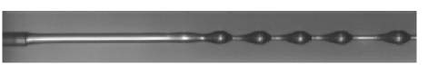
Figure 1: An annular film of viscous fluid flowing down the outside of a thin nylon fiber; the surrounding fluid is air. Note that the figure has been rotated by 90${}^{\text{o}}$ with gravity acting towards the right. Perturbations develop along the free surface some distance down the fiber; once formed, these perturbations continue to travel down the fiber. Image length = 9.7 cm.

A related problem to annular films is on the motion of cylindrical jets, which in contrast have no fixed internal boundary. Analytical studies on the motion and stability of inviscid and viscous jets dates back to the work of Plateau plat73 , Lord Rayleigh ray1879 ; ray1892 , Weber weber31 and Chandrasekhar chan61 . It is known that capillary effects drive perturbation growth along the jet free surface, often referred to as the Plateau-Rayleigh instability. Analytical results developed from temporal linear stability theory chan61 were tested in experiments by Donnelly & Glaberson donn66 , who found strong (fair) quantitative agreement between the theoretical and measured dispersion relation for an inviscid (viscous) jet. The dynamics of free surface perturbations along cylindrical jets and annular films are, however, quite different. In the cylindrical case jet breakup occurs when the perturbations become sufficiently large donn66 , while in the annular case the large amplitude perturbations remain connected by a liquid film cras06 ; duprat07 ; kliak01 .

Recently, several theoretical studies have analyzed the temporal linear stability of an annular viscous film flowing down a vertical fiber in the Stokes cras06 ; kliak01 and moderate Reynolds number trif92 ; sisoev06 limits; the base flow in these studies is assumed to be a steady, unidirectional parallel flow. Here we test these results by determining whether: (i) the base flow used in cras06 ; kliak01 ; trif92 ; sisoev06 matches the experimental flow; and (ii) the dispersion relations derived in the Stokes and moderate Reynolds number limits cras06 ; sisoev06 correctly predict the nascent growth of perturbations measured in low and moderate Reynolds number flows.

As free surface perturbations travel down a vertical fiber, many interesting phenomena occur duprat07 ; cras06 ; kliak01 ; sisoev06 . In experiments, Kliakhandler, Davis and Bankoff (KDB) observed three types of behavior far down the length of the fiber ($\approx$ 2 m) kliak01 . At the highest flow rate (regime a), the film between perturbations is thick and uniform, and faster moving perturbations collide into slower moving perturbations (unsteady behavior). At an intermediate flow rate (regime b), the spacing, size and speed of the perturbations is constant so that no collisions occur (steady behavior). And at the lowest flow rate (regime c), the fluid periodically drips from the tank, rather than jets as with the higher flow rates, creating a regular spacing between perturbations near the tank outlet. The long time between drips allows the film connecting consecutive perturbations to thin and subsequently become unstable to smaller capillary perturbations. (Figure 1 in kliak01 illustrates these three regimes of behavior.) Simulations of a Stokes flow model developed by KDB qualitatively captured two of the three observed behaviors (regimes b and c), while the behavior associated with the highest flow rate (regime a) could not be replicated kliak01 .

Craster & Matar (CM) cras06 select a different scaling than KDB to derive an evolution equation for the free surface. Using traveling wave solutions, their Stokes flow model quantitatively predicted the perturbation speed and height of regime a measured by KDB. The model also qualitatively captured regime c, though the steady pattern of perturbation spacing found in regime b could not be matched with traveling wave solutions. In experiments, CM observed regime b near the tank outlet, however, they found the regularly spaced pattern of perturbations disassembled itself further down the fiber. From this observation, CM concluded regime b is a transient rather than steady regime cras06 .

The contradiction in observations of regime b (steady behavior) by KDB and CM motivated us to look more closely at the steady and unsteady states by examining the dynamics of the perturbations where they initially form along the fiber. In experiments using fluids with different densities, surface tensions and viscosities we observe regimes a (unsteady), b (steady) and c (dripping) as described by KDB kliak01 , though the focus of this paper is on regimes a and b. In our experiments, we observe the flow transitions abruptly from unsteady to steady behavior at a critical flow rate $Q_{c}$ (the value of $Q_{c}$ is dependent on the particular fluid) smolka06 . In a recent independent study, Duprat et al. duprat07 explain the transition from regime a (unsteady behavior) to regime b (steady behavior) as a transition from a convective to absolute instability. In their experiments with silicone oil using a range of fiber and orifice radii, they find the transition occurs only at intermediate film thicknesses and for sufficiently small fiber radii; at thin or thick film thickness, they find the perturbation behavior remains convective (unsteady) duprat07 . These criteria may explain why CM did not observe the steady dynamics of regime b in their experiments with silicone oil. Here we find the transition from unsteady to steady behavior is also correlated to the rate at which perturbations naturally form along the fiber. For $Q<Q_{c}$ (steady case), the rate of perturbation formation is constant. As a result the position along the fiber where perturbations form is nearly fixed, and the spacing between consecutive perturbations remains constant as they travel 2 m down the fiber. For $Q>Q_{c}$ (unsteady case), the rate of perturbation formation is modulated. As a result the position along the fiber where perturbations form oscillates irregularly, and the initial speed and spacing between perturbations varies resulting in the coalescence of neighboring perturbations further down the fiber.

The paper is organized as follows. The experimental setup and properties of the unperturbed flow are presented in Section II. Measurements of the perturbation growth are compared to analytical predictions for Stokes and moderate Reynolds number conditions in Section III. The perturbation behavior exhibited in regimes a (unsteady) and b (steady) near the tank outlet is closely examined in Section IV. Conclusions are provided in Section V.

II Experimental Setup & Details

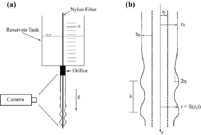
Figure 2: (a) Schematic of experimental setup. (b) Cross-section of an annular film flowing down the outside of a fiber of radius $r_{f}$ (not to scale). The unperturbed film radius measured from the fiber centerline is $r_{0},$ unperturbed film thickness $h_{0}$, perturbation amplitude $\eta(z,t)$ and perturbation wavelength $\lambda$.

II.1 Experimental Apparatus

The experimental setup consists of viscous fluids, a reservoir tank/orifice assembly, nylon fishing line, a high-speed digital imaging camera, illumination, a computer and edge-detection software (a schematic of the experiment is shown in Figure 2(a)). The reservoir tank (6 L capacity) is graduated at 100 mL increments to measure flow rate. An orifice, machined with a flat edge (inner radius = 0.11 cm, outer radius = 0.16 cm, length = 2.6 cm), is attached to the bottom of the tank to ensure a reproducible solid/fluid/air contact line in the experiment. A nylon fiber ($r_{f}=0.029$ cm) anchored from above, passes through the center of the tank/orifice assembly, and is held vertically plumb with weights attached 2 m below the orifice. The fluid, which is gravitationally forced from the tank, coats the fiber to create an annular film. To reduce air currents and other noise during data collection, the entire apparatus is enclosed by an aluminum frame with plastic sheet sidewalls and top.

The motion of the annular film is recorded using a high-speed digital imaging camera (Phantom v4.2) at rates between 1000-4000 frames/s and an image size of 64 x 512 pixels² with the camera focused on approximately the upper 10 cm of the fiber. Illumination is obtained using silhouette photography following scor90 , with a 250 W lamp, an experimental grade one-way transparent mirror (Edmund Scientific, A40,047) and high contrast reflective screen material (Scotchlite 3M 7615). Movies of the annular film are recorded and downloaded to a computer using camera software. The free surface of the film is determined from movie images using an edge-detection algorithm. The algorithm locates the free surface by interpolating the maxima positions in a gradient image; the gradient image is produced using the Frei-Chen operator frei77 . The algorithm can detect the edge of the film free surface to within approximately 1/10${}^{\text{th}}$ of a pixel which for the screen resolution in our experiments corresponds to $\approx 0.002$ cm.

The experimental fluids consist of castor oil, vegetable oil (Crisco) and an 80:20 glycerol/water solution (by weight). The temperature, density ($\rho$), surface tension ($\gamma$), dynamic viscosity ($\eta$) of the fluids, and the framing rate and screen resolution used in the experiments are listed in Table 1. The surface tension was measured at room temperature using a Fisher 21 tensiomat and viscosity was measured using a temperature controlled cone and plate rheometer (Brookfield, Model DV-III+). The fluid temperature varied by less than 4.6%, 1.9% and 1.4% in the castor oil, vegetable oil and glycerol solution experimental runs, respectively. We note that the selection of fluids allows us to independently probe the influence of surface tension or viscosity on flow behavior since castor oil and vegetable oil have comparable surface tension while vegetable oil and the glycerol solution have comparable viscosity.

Table 1: Fluid properties and experimental conditions.

Fluid	Temp.	$\rho$	$\gamma$	$\mu$	Framing	Screen
					Rate	Resolution
	oC	$\frac{\text{g}}{\text{cm}^{3}}$	$\frac{\text{dyn}}{\text{cm}}$	$\frac{\text{g}}{\text{cm}\cdot\text{s}}$	$\frac{\text{frames}}{\text{s}}$	$\frac{\text{cm}}{\text{pixel}}$
Castor Oil	21.9	0.94	36.8	8.48	1000	0.0190
Vegetable Oil	21.6	0.92	34.3	0.58	4000	0.0180
Glycerol Solution	21.2	1.21	60.4	0.54	2000	0.0186

II.2 Base Flow Properties

In each experiment, the reservoir tank drained under the influence of gravity and the elapsed time and tank volume were recorded as the fluid passed each 100 mL mark to determine the flow rate ($Q$). Data was collected only while the flow was jetting from the orifice and an unperturbed region of the film free surface was present near the orifice (corresponding to regimes a and b kliak01 ). Measurements of the flow rate during each experimental run for vegetable oil (square), glycerol solution (triangle) and castor oil (circle), is shown in Figure 3(a). (Note that in each experiment the flow rate decreases as the tank volume decreases.) Figure 3(a) shows that the flow rate increases linearly over the range of tank volume used in each experimental run. Furthermore, the flow rate decreases with increasing viscosity ($Q_{castor}$ is an order of magnitude less than $Q_{glycerol}$ and $Q_{vegetable}$), and increases with increasing surface tension ($Q_{glycerol}>Q_{vegetable}$).

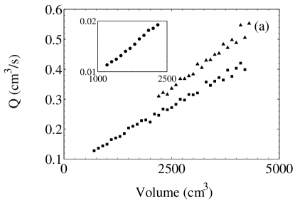
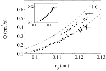
Figure 3: (a) Experimental flow rate as a function of the reservoir tank volume. (b) Flow rate as a function of the unperturbed film radius: experimental data (symbols), theory given by (4) with $r_{f}=0.029$ cm (dotted); bars represent the resolution of experimental measurements. Symbols correspond to: vegetable oil (square), glycerol solution (triangle) and castor oil (circle).

The unperturbed film radius $r_{0}$, measured from the fiber centerline to the unperturbed free surface (see Figure 2(b)), was measured using edge-detection software. Figure 3(b) shows the unperturbed radius increases with flow rate in each experimental run. This trend is similar to behavior observed in dip coating in which the film thickness increases with the velocity at which the fiber is drawn from the fluid source at sufficiently low withdrawal rates quere99 ; ruck02 ; deryck96 ; shen02 . Comparing data for the glycerol solution (triangle) and vegetable oil (square) experiments, we find that at a fixed flow rate higher surface tension (glycerol solution) results in a thinner unperturbed film. In our experiments, the range of the ratio of unperturbed film thickness to fiber radius is $\,2.5<h_{0}/r_{f}<3.3,\,$ which means the films are thick.

The relevant forces that characterize the dynamics of an annular film can be determined by considering two dimensionless groups, the Reynolds number and Bond number. Following CM cras06 , we define characteristic length and velocity scales as

$$\mathcal{L}=\gamma/(\rho gr_{0}),\qquad\mathcal{V}~{}=~{}\rho gr_{0}^{2}/\mu,$$ (1)

where $g$ is the gravitational constant of acceleration, the Reynolds number as $\text{Re}=\rho\mathcal{VL}/\mu,$ which compares inertial to viscous effects, and the Bond number as $\text{Bo}=\rho gr_{0}^{2}/\gamma,$ which compares gravitational to surface tension effects cras06 . The values of Re and Bo for our experiments, listed in Table 2, indicate inertial effects are negligible for castor oil $(\text{Re}\sim O(10^{-2})),$ in contrast to the vegetable oil and glycerol solution experiments $(\text{Re}\sim O(10)),$ and surface tension dominates over gravitational effects in the formation of interfacial perturbations for all three fluids $(\text{Bo}\sim O(10^{-1})).$

Table 2: The Reynolds number and Bond number measured in experiments.

Fluid	Re	Bo
Castor Oil	0.049 - 0.054	0.26 - 0.32
Vegetable Oil	9.4 - 11.6	0.26 - 0.40
Glycerol Solution	27.2 - 31.2	0.23 - 0.30

Experimental cras06 ; kliak01 and theoretical cras06 ; kliak01 ; sisoev06 ; trif92 studies often assume the base flow of an annular film is steady, unidirectional and parallel. Under these conditions, the unperturbed flow with free surface located at $r=r_{0}$ and constant pressure field $p(r,z,t)=p_{0}$ is described by the boundary value problem for the axial velocity $w(r)$

$$\mu r^{-1}\partial_{r}(r\partial_{r}w)+\rho g=0,\quad w(r_{f})=0,\quad\partial_{r}w(r_{0})=0,$$ (2)

where the boundary conditions include no-slip at the fiber and zero tangential stress at the free surface. Eqs. (2) can be solved exactly for the axial velocity to obtain

$$w(r)={\rho g\over 4\mu}\left[2r_{0}^{2}\ln(r/r_{f})+r_{f}^{2}-r^{2}\right].$$ (3)

Using (3), the flow rate of an annular film can be expressed in terms of $r_{f}$ and $r_{0}$

$$Q(r_{f},r_{0}) = 2\pi\int_{r_{f}}^{r_{0}}rw(r)\,dr$$ (4)

$$= {\rho g\pi\over 8\mu}\left(4r_{f}^{2}r_{0}^{2}+4r_{0}^{4}\ln(r_{0}/r_{f})-r_{f}^{4}-3r_{0}^{4}\right).$$

By comparing (4) to experimental data, we can test the assumption that the base flow of an annular film is a steady, unidirectional parallel flow.

Figure 3(b) shows a comparison of the flow rate as a function of the unperturbed film radius for vegetable oil, glycerol solution and castor oil measured directly in experiments (symbols) and using (4) with $r_{f}=0.029$ cm (dotted line). We find excellent agreement between (4) and the experimental data in the castor oil (circle) and vegetable oil (square) experiments which indicates the flow in these experiments is well approximated by a unidirectional parallel flow. The theory overestimates $Q$ by as much as 12% in the glycerol solution experiment (triangle). This is not surprising since the assumptions on the flow are equivalent to steady Stokes flow. With $\text{Re}\approx 30,$ we suspect the Stokes flow assumption is not valid for the glycerol solution experiment. Based on the comparison in Figure 3(b), we estimate (3) and (4) are valid when $\text{Re}\leq 10.$ The experiments conducted by KDB kliak01 and CM cras06 meet this criterion, thus we conclude their assumption that the flow is steady, unidirectional and parallel is indeed valid.

In the proceeding sections, we examine the dynamics of a perturbed annular film including the initial formation and longer-time dynamics of interfacial perturbations along the free surface.

III Perturbation Growth

The image in Figure 1 illustrates the capillary instability an annular viscous film undergoes as the unperturbed free surface becomes unstable to undulations that develop into large amplitude perturbations. Next we present experimental observations on the growth of these interfacial perturbations and compare their initial growth to theoretical predictions developed from linear stability analysis. Before proceeding, we first recount relevant stability results developed in the Stokes cras06 and moderate Reynolds number flow sisoev06 limits.

III.1 Linear Stability Results

III.1.1 Stokes Flow

Craster & Matar cras06 derive a long-wave Stokes flow evolution equation for the free surface of the annular film, $r=S(z,t),$ under the assumption that the unperturbed film radius $r_{0}$ is small relative to the capillary length $l_{c}=\gamma/\rho gr_{0}$ (i.e., $\text{Bo}=r_{0}/l_{c}=\rho gr_{0}^{2}/\gamma\ll 1$) and the Reynolds number is sufficiently small ($\text{Re}\leq O(1)$), to obtain

$$\partial_{\hat{t}}(\hat{S}^{2})+{1\over 8}\partial_{\hat{z}}\left[\left[\partial_{\hat{z}}\left({1\over\hat{S}}-(\text{Bo})^{2}\partial_{\hat{z}\hat{z}}\hat{S}\right)-1\right]\times(\alpha^{4}-4\hat{S}^{2}\alpha^{2}+3\hat{S}^{4}-4\hat{S}^{4}\ln(\hat{S}/\alpha))\right]=0,$$ (5)

where $\hat{S},\hat{z},\hat{t}$ are dimensionless variables satisfying the scalings

$$S=r_{0}\hat{S},\qquad z=\mathcal{L}\hat{z},\qquad t=\mathcal{L}\hat{t}/\mathcal{V},$$ (6)

and $\alpha=r_{f}/r_{0}.$ Conducting a linear stability analysis by perturbing about the base flow

$$\hat{S}(\hat{z},\hat{t})=1+\hat{S}_{1}e^{(im\hat{z}+\sigma\hat{t})},$$ (7)

where $m$ is the (real) dimensionless wavenumber and $\sigma$ is the (complex) dimensionless growth rate CM obtain the following dispersion relation for the growth rate

$$\sigma={m^{2}\over 16}(\text{Bo}^{2}m^{2}-1)(\alpha^{4}-4\alpha^{2}+3+4\ln(\alpha))$$

$$-{im\over 2}\left(\alpha^{2}-1-2\ln(\alpha)\right).$$ (8)

III.1.2 Moderate Reynolds Number Flow

In an analytical study, Trifonov trif92 derived model equations for fluid flowing down the inside or outside of a vertical cylinder at moderate Reynolds number; the model includes evolution equations for the film thickness, $h(z,t)=S(z,t)-r_{f},$ and volumetric flow rate, $q(z,t)$. In a recent study, Sisoev at al. sisoev06 rescale Trifonov’s equations for flow down the outside of a vertical cylinder, casting the model in terms of a generalized falling film model shka04 (see Eqs. (11)-(13) in sisoev06 ). Conducting a linear stability analysis of the rescaled equations by perturbing about the base solution

$$\hat{h}(\hat{z},\hat{t}) = 1+\hat{h}_{1}e^{i(m\hat{z}-\sigma\hat{t})},$$ (9a)

$$\hat{q}(\hat{z},\hat{t}) = 1+\hat{q}_{1}e^{i(m\hat{z}-\sigma\hat{t})},$$ (9b)

where $m$ is the (real) dimensionless wavenumber and $\sigma$ is the (complex) dimensionless growth rate, Sisoev et al. obtain a dispersion relation for $\sigma$ satisfying

$$\sigma^{2}+(ia_{1,0}-a_{1,1}m)\sigma+{m\over 1+\varepsilon}(-a_{0,3}m^{3}-a_{0,1}m+ia_{0,0})=0,$$ (10)

where $\varepsilon=h_{0}/r_{f}$ and the constant coefficients $a_{1,0},a_{1,1},a_{0,3},a_{0,1},a_{0,0}$ are defined in the Appendix. The variables $\hat{h},\hat{z},\hat{t}$ are dimensionless quantities satisfying the scalings

$$h=h_{0}\hat{h},\qquad z={h_{0}\over\kappa}\hat{z},\qquad t={h_{0}\over\kappa U}\hat{t},$$ (11)

where

$$\kappa=\left({\rho gh_{0}^{2}\over\gamma}\right)^{1/3},\qquad U={Q\over 2\pi r_{f}h_{0}},$$ (12)

represent a stretching parameter and characteristic velocity scale, respectively. We note that the long-wave model used by Sisoev et al. was derived under the assumption that $\kappa^{2}\ll 1.$

The stability results developed by Craster & Matar cras06 and Sisoev at al. sisoev06 are temporal analysis (since $m\in{\mathbb{R}}$ and $\sigma\in{\mathbb{C}}$), and thus model the case in which interfacial perturbations grow in amplitude everywhere along the film keller73 . Our interest is in testing these stability predictions by comparing the theoretical dispersion relations (8) and (10) to the growth rate of perturbations measured in experiments conducted in the Stokes and moderate Reynolds number flow limits.

III.2 Experimental Observations of Perturbation Formation

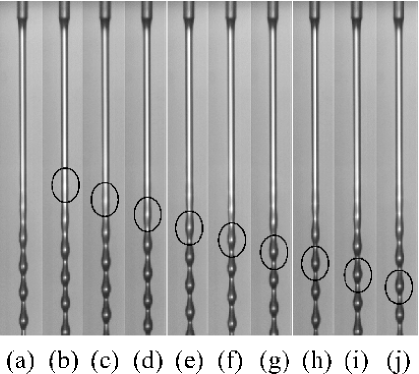
Figure 4: An annular film of castor oil flowing down the outside of a thin nylon fiber. The film loses uniformity approximately 5.4 cm from the orifice indicated by the circled area in frame (b). Subsequent frames track the position and growth of this nascent perturbation. Time between images is 0.42 s and elapsed time = 3.7 s. Image height = 9.7 cm.

Figure 4 shows a series of images tracking the formation of a perturbation along an annular film of castor oil. In frame (b), a small amplitude perturbation first appears along the film approximately 5.4 cm from the orifice (circled region). Frames (c)-(j) track the position of this perturbation as it grows in amplitude and saturates in size. Once formed, the perturbation continues moving down the fiber (not shown). Since the perturbation grows in amplitude as it travels down the fiber, the flow is spatially (convectively) unstable rather than temporally (absolutely) unstable to perturbations keller73 .

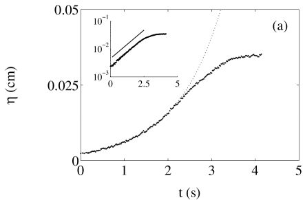
Figure 5: (a) Amplitude ($\eta$) and (b) wavelength ($\lambda$) of a nascent perturbation as a function of time for castor oil ($Q=0.0194$ cm³/s); experimental data corresponds to the perturbation tracked in Figure 4. (a) The initial amplitude growth of the perturbation is exponential (shown in inset on log-linear scale) followed by nonlinear saturation. Dotted line: fit of data to $\eta(t)=0.0023e^{0.959t}$ corresponding to growth between frames (b)-(g) in Figure 4. (b) The wavelength decreases during the time interval that the amplitude grows exponentially and then saturates in length as the amplitude saturates in size.

To characterize the growth of a perturbation we measure the amplitude $\eta$ (half the radial distance from first minima to first maxima) and the wavelength $\lambda$ (the axial distance from first to second maxima) as shown in Figure 2(b) using edge-detection software; both measurements are made in the moving reference frame of the perturbation. The data shown in Figure 5 corresponds to the perturbation followed in Figure 4. Figure 5(a) shows the nascent growth of the amplitude is exponential (inset) followed by a slower phase as the perturbation saturates in size ($\eta_{saturate}=0.035$ cm). The growth rate for the initial formation of the amplitude is determined from a least squares fit of the data to an exponential function yielding the dimensional growth rate $\sigma_{dim}=0.959$ s^-1 (fit indicated by dotted line in Figure 5(a)). The wavelength of this perturbation decreases from $\lambda=0.98$ cm to 0.80 cm during the time interval that the amplitude grows exponentially $(0\leq t\leq 2.34~{}\text{s})$, before saturating in length to $\lambda=0.83$ cm, as shown in Figure 5(b). The decrease in $\lambda$ during the exponential phase of growth indicates the annular film is unstable to a range of wavenumbers ($=2\pi/\lambda),$ rather than to one fixed value.

The behavior displayed in Figure 5 for the amplitude and wavelength is typical of observations made in the castor oil, vegetable oil and glycerol solution experiments. Comparison of perturbation growth to the Stokes (8) or moderate Reynolds number (10) dispersion relations depend on the flow conditions in each experiment, specifically on the Reynolds and Bond numbers (provided in Table 2). In the castor oil experiments, $\text{Bo}\sim O(10^{-1})$ and $\text{Re}\sim O(10^{-2}),$ thus satisfying the requirements of the Stokes model ($\text{Bo}\ll 1,$ $\text{Re}\leq O(1)$). Since $\text{Re}\approx 30$ in the glycerol solution experiments, inertial effects cannot be ignored, and so we compare this case to the moderate Reynolds number model. With $\text{Bo}\sim O(10^{-1})$ and $9.4<\text{Re}<11.6,$ the vegetable oil experiments are on the border of the requirements for the Stokes model. In this case we compare the experimental data to both the Stokes and moderate Reynolds number dispersion relations.

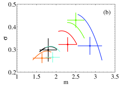
Figure 6: (Color online) Dimensionless growth rate as a function of dimensionless wavenumber for experiments with (a) castor oil and (b) vegetable oil. Circles correspond to experimental data of the average growth rate and wavenumber measured over several perturbations at (a): Q = 0.0194 - orange, 0.0171 - black, 0.0148 - cyan, 0.0123 - red, 0.0111 - green and 0.0103 - blue (cm³/s); (b): Q = 0.416 - orange, 0.383 - black, 0.342 - cyan, 0.252 - red, 0.211 - green and 0.170 - blue (cm³/s). Vertical bars represent the standard deviation of $\sigma$ and horizontal bars represent the range of $m$ measured during the period of exponential growth over all perturbations measured. Corresponding colored curves represent theoretical prediction given by the Stokes flow dispersion relation (8) of ${\mathcal{R}e}(\sigma)$ plotted over the range of $m$ measured in experiments cras06 .

Figure 6 shows a comparison of the measured amplitude growth rate to the dispersion relation developed by Craster & Matar in the Stokes flow limit (8) for (a) castor oil and (b) vegetable oil at various flow rates. At a given flow rate, the growth rate for several perturbations was measured (8-12 perturbations for castor oil, and 15-44 for vegetable oil). The average dimensionless growth rate ($\sigma=\sigma_{dim}\mathcal{L}/\mathcal{V}$) and dimensionless wavenumber ($m=2\pi\mathcal{L}/\lambda$) measured over all the perturbations is denoted by a circle with each color corresponding to a different flow rate. The vertical bars represent the standard deviation of all the growth rates measured at a given flow rate during the period of exponential growth. Since the perturbation wavelength decreases over a range of values during the exponential phase of growth, we cannot assign a single wavenumber to its growth. Instead, the horizontal bars represent the range of wavenumber measured during the period of exponential growth of all the perturbations. The corresponding colored curves represent the real part of the growth rate predicted by (8) plotted over the range of wavenumber measured at each flow rate. We consider the theory to be in agreement with the experimental data (at a given flow rate) if the theoretical curve overlaps the rectangular region defined by the resolution bars of the data. Figure 6 shows that the Stokes theory is in agreement with four of the six castor oil experiments and with five of the six vegetable oil experiments. In the other three experiments, the theory overestimates the measured values by 10 to 13 %. The quantitative agreement between theory and experimental data is excellent, a significant result considering: (i) the comparison is between a temporal stability theory and a spatial instability of the film, and (ii) the value of the Reynolds number in the vegetable oil experiments, $\text{Re}\approx 10,$ is slightly higher than the criteria for the Stokes theory, $\text{Re}\leq O(1).$

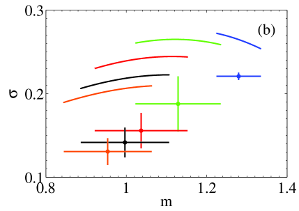
Figure 7: (Color online) Dimensionless growth rate as a function of dimensionless wavenumber for experiments with (a) vegetable oil and (b) glycerol solution. Circles correspond to experimental data of the average growth rate and wavenumber measured over several perturbations at (a): Q = 0.416 - orange, 0.383 - black, 0.342 - cyan, 0.252 - red, 0.211 - green and 0.170 - blue (cm³/s); (b): Q = 0.538 - orange, 0.493 - black, 0.437 - red, 0.381 - green and 0.325 - blue (cm³/s). Vertical bars represent the standard deviation of $\sigma$ and horizontal bars represent the range of $m$ measured during the period of exponential growth over all perturbations measured. Corresponding colored curves represent theoretical prediction given by the moderate Reynolds number flow dispersion relation (10) of ${\mathcal{I}m}(\sigma)$ plotted over the range of $m$ measured in experiments sisoev06 .

Figure 7 shows a comparison of the measured amplitude growth rate to the dispersion relation developed by Sisoev et al. in the moderate Reynolds number limit (10) for (a) vegetable oil and (b) glycerol solution at various flow rates. The data and theory are presented in a similar fashion to Figure 6 with the exception that the dimensionless growth rate and wavenumber are given by $\sigma=\sigma_{dim}h_{0}/(\kappa U)$ and $m=2\pi h_{0}/(\kappa\lambda)$, and the growth rates for the glycerol solution experiments are averaged over 88 to 102 perturbations. We recall that the moderate Reynolds number model is valid as long as $\kappa^{2}\ll 1$; in all of the experiments shown in Figure 7, $\kappa^{2}\sim O(10^{-1}).$ We find the moderate Reynolds number model overestimates the measured growth rates by 28 to 50 % in the vegetable oil experiments and 15 to 48 % in the glycerol solution experiments, as shown in Figure 7. Clearly, the Stokes model is more accurate at predicting the growth rate of the perturbations in the vegetable oil experiments than the moderate Reynolds number model. This is somewhat surprising since the vegetable oil experiments slightly exceed the Reynolds number limit of the Stokes model, but satisfy the assumption on $\kappa^{2}$ for the moderate Reynolds number model. While the theoretical growth rates in Figure 7 are on the same order of magnitude as the measured values, the quantitative match between theory and data is not strong.

We note that the range of the measured amplitude growth rate in experiments (indicated by the vertical bars in Figures 6 & 7) varies by fluid and flow rate. For castor oil (Figure 6(a)), the range is fairly small which we attribute to the low Reynolds number ($\text{Re}\sim O(10^{-2})$) in the experiments. For the experiments with vegetable oil (Figures 6(b) and 7(a)) and glycerol solution (Figure 7(b)) with $Q>0.345$ cm³/s, the range of the measured amplitude growth rates is large. Naively, one could attribute this to the higher Reynolds number in these experiments ($10\lesssim\text{Re}\lesssim 30$). This is, however, not the complete picture. Notice the range is significantly smaller for the glycerol solution experiment at $Q=0.325$ cm³/s (blue (rightmost) data set in Figure 7(b)). The difference in this data set compared to the other glycerol solution and vegetable oil sets is in the behavior of the perturbations. The perturbation behavior in the sets with a large range of amplitude growth rates is unsteady, while the behavior in the blue glycerol solution data set is steady. (The notion of unsteady and steady perturbation behavior will be explained in detail in Section IV.) Therefore, we find the range of amplitude growth rate of the perturbations is correlated to both the Reynolds number of the flow and the longer-time dynamics of the perturbations.

Next, we examine the dynamics of perturbations after their initial formation and explain a physical mechanism that controls a known transition in the flow from unsteady to steady perturbation behavior.

IV Steady and Unsteady Perturbation Dynamics

The dynamics of interfacial perturbations along an annular film flowing down a vertical fiber can be broken down into three essential stages: (i) initial exponential growth of the perturbation amplitude accompanied by a decrease in wavelength; (ii) nonlinear saturation of the perturbation amplitude and wavelength; and (iii) longer-time behavior in which the perturbation wavelength may (unsteady - see Figure 1) or may not (steady) vary along the fiber; this last stage has been noted in other experimental studies cras06 ; duprat07 ; kliak01 . Here we explain a physical mechanism that controls this third stage of dynamics.

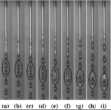
Figure 8: Coalescence of two perturbations along an annular film of glycerol solution. $Q~{}=~{}0.359~{}$cm³/s, time between images is 0.0125 s, elapsed time = 0.1 s, image height = 9.7 cm.

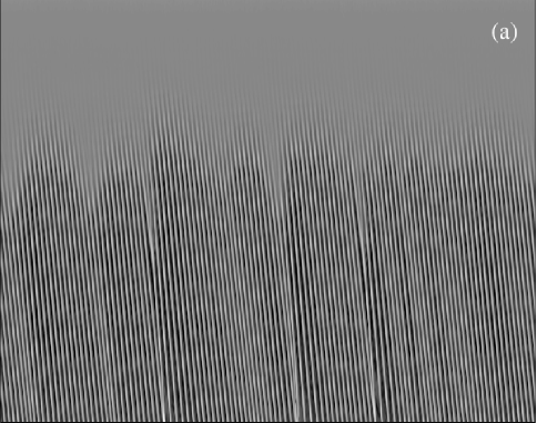
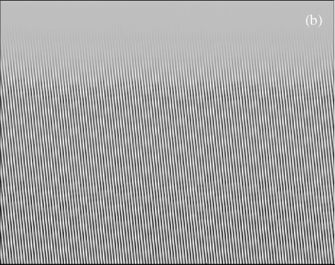
Figure 9: Space-time plot illustrating the motion of perturbations along a vertical fiber during (a) unsteady and (b) steady behavior. Lighter (darker) regions correspond to thicker (thinner) regions of the fluid interface with light characteristic lines indicating the location of perturbations along the fiber as a function of time. Experimental fluid: glycerol solution ($Q_{c}=0.345$ cm³/s), (a) $Q=0.347~{}$cm³/s, (b) $Q=0.336~{}$cm³/s, elapsed time = 8.09 s, image height = 8.22 cm. The top of each image is 0.58 cm below the orifice.

In experiments with all three fluids, we observe the perturbation motion abruptly transitions from unsteady (regime a) to steady (regime b) behavior at a critical flow rate, $Q_{c}$ ($Q_{c}=$ 0.0095 cm³/s for castor oil, 0.119 cm³/s for vegetable oil and 0.345 cm³/s for glycerol solution) smolka06 , similar to observations made by Duprat et al. in their experiments with silicone oil duprat07 . Following KDB kliak01 , we define the flow to be steady if no perturbations coalesce as they travel down the full length of the fiber ($\approx$ 2 m), and unsteady otherwise while the flow is jetting from the orifice. An example of unsteady behavior in which two perturbations coalesce is shown in Figure 8. Note: we will not be examining the dripping state, regime c kliak01 , which occurs at a lower flow rate, $Q_{drip}<Q_{c}$. We find the transition from unsteady ($Q>Q_{c}$) to steady ($Q_{drip}<Q<Q_{c}$) behavior is robust in the sense that once an experiment transitions to steady behavior (as the flow rate decreases) it does not revert back to the unsteady state.

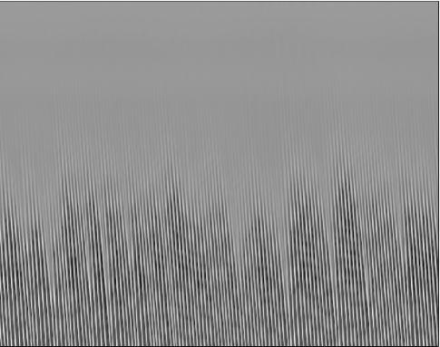
Figure 10: Space-time plot illustrating the motion of perturbations along a vertical fiber during unsteady behavior. Experimental fluid: glycerol solution; $Q=0.516~{}$cm³/s, elapsed time = 8.09 s, image height = 8.22 cm. The top of the image is 0.58 cm below the orifice.

The space-time plots in Figure 9 illustrate (a) unsteady and (b) steady perturbation behavior for experiments with glycerol solution. Each plot is focused on 8.22 cm of the film, with the top of each plot located 0.58 cm below the orifice; the time span of each plot is 8.09 s. The plots are created by mapping the radius of the free surface of the film, $r=S(z,t),$ to a gray level with lighter (darker) gray level corresponding to thicker (thinner) regions of the free surface. The light characteristic lines in the plots indicate the location of perturbations as they move down the fiber, and their slope represent the speed of the perturbations. Two features in the space-time plots distinguish the unsteady and steady perturbation behavior. First, the location along the fiber that perturbations form (which we refer to as the boundary) oscillates irregularly in the unsteady case and appears nearly fixed in the steady case smolka06 . Second, in the unsteady case perturbations coalesce as faster moving perturbations collide into slower moving perturbations (indicated by intersecting characteristic lines), whereas in the steady case perturbations do not coalesce as they travel with the same terminal speed down the fiber (indicated by parallel characteristic lines) kliak01 ; smolka06 . The longer-time motion of the perturbations appears to be correlated to the motion of the boundary. Notice in Figure 9(a) that large spatial variations in the boundary modulate the perturbation speed (i.e., the slope of the characteristic lines) which results in coalescence events later down the fiber. In the steady case, there is no spatial variation in the boundary, and as a result, the perturbations remain equally spaced as they travel with constant terminal speed down the full length of the fiber (not shown in Figure 9(b)). Our observations of the steady case (regime b) are consistent with those of KDB kliak01 . Given the robustness of the steady dynamics in all of our experiments, we conclude this is not a transient state as CM report cras06 . Finally, we note that when the flow is unsteady, the oscillation frequency of the boundary increases with increasing flow rate; for example, compare the boundary frequency in Figures 9(a) and 10.

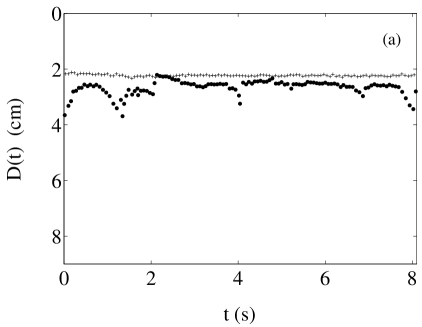
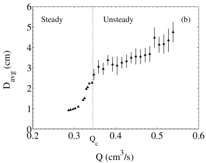
Figure 11: (a) The distance from the orifice ($D$) where perturbations initially form along the fiber (i.e., the location of the boundary) as a function of time, corresponding to the data shown in Figure 9(a) for the unsteady case at $Q=0.347~{}$cm³/s ($\bullet$) and in Figure 9(b) for the steady case at $Q=0.336~{}$cm³/s (+). (b) Average distance ($D_{\text{avg}}$) from the orifice that perturbations form as a function of flow rate $Q$ for experiments with glycerol solution. Vertical bars represent the standard deviation of $D$ over all the perturbations measured at a given flow rate. The dotted vertical line denotes the transition flow rate separating steady and unsteady perturbation behavior.

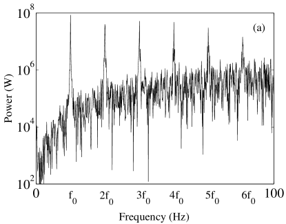
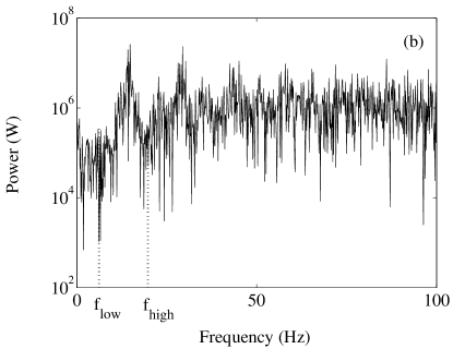
Figure 12: Power spectrum of the distance from the orifice $D$ that perturbations form as a function of time. Plots correspond to the data shown in Figure 11(a) in: (a) steady behavior ($+$) at $Q=0.336$ cm³/s and (b) unsteady behavior ($\bullet$) at $Q=0.347$cm³/s for glycerol solution. In the steady case, the fundamental frequency $f_{0}$ = 14.45 Hz, is the first harmonic in the power spectrum. In the unsteady case, the bandwidth supporting the fundamental peak is larger than the steady case.

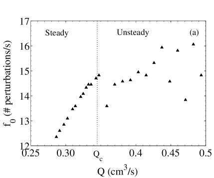
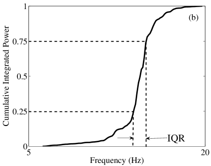
Figure 13: (a) Fundamental frequency as a function of flow rate measured from power spectra of $D$ versus $t$ data in experiments with glycerol solution. The dotted vertical line denotes the transition flow rate separating steady and unsteady perturbation behavior. (b) The (normalized) cumulative integrated power measured within the support of the first peak between f${}_{\text{low}}=6.18$ Hz and f${}_{\text{high}}=19.77$ Hz for the spectra shown in Figure 12(b). The Interquartile Region (IQR) is the frequency bandwidth bounding the middle 50% of the cumulative integrated power.

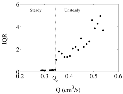
Figure 14: Interquartile Region (IQR), or frequency bandwidth, as a function of flow rate for the glycerol solution experiments. An abrupt transition in the bandwidth occurs at the transition flow rate, $Q_{c}$.

To characterize the motion of the boundary, we measure the distance from the orifice $D$ that each perturbation initially forms along the fiber (at a fixed flow rate) using edge-detection software; a perturbation is detected when its amplitude ($\eta$) initially exceeds 1/10${}^{\text{th}}$ of a pixel or $\approx$ 0.002 cm. The data shown in Figure 11(a) corresponds to the space-time plots of the unsteady ($\bullet$) and steady ($+$) experiments shown in Figure 9. Figure 11(b) is a plot of the average distance from the orifice that perturbations form ($D_{\text{avg}}$) as a function of flow rate in experiments with glycerol solution. The vertical bars represent the standard deviation of $D$ over all the perturbations measured at a fixed flow rate and the dotted vertical line represents the transition flow rate, $Q_{c}.$ The distance that perturbations form from the orifice increases monotonically with increasing flow rate. In the steady case, at a given flow rate the distance is nearly constant, whereas in the unsteady case, the range of distance that perturbations form increases with increasing flow rate. These results are consistent with experimental observations made by Duprat et al. duprat07 .

To understand the physical mechanism controlling the steady and unsteady states we examine the power spectra of $D(t)$ in the glycerol solution experiments. Figures 12(a) and (b) represent the power spectra for the steady ($+$) and unsteady ($\bullet$) perturbation behavior shown in Figure 11(a). In the steady case the fundamental frequency ($f_{0}$), which is the first harmonic of the power spectra, represents the rate at which perturbations form along the fiber (e.g., $f_{0}=14.45$ perturbations/s in the experiment shown in Figure 9(b)); in the unsteady case the fundamental peak is much broader so that $f_{0}$ is less well defined. As a function of increasing flow rate, the fundamental frequency (i.e., rate of perturbation formation) increases linearly when the perturbation dynamics are steady ($Q<Q_{c}$), and is scattered about $\approx 15$ perturbations/s when the dynamics are unsteady ($Q>Q_{c}$) (see Figure 13(a)). Another feature in the power spectra distinguishing steady and unsteady behavior is in the frequency bandwidth supporting the fundamental peak; the bandwidth of the unsteady spectra is larger than the steady spectra in Figure 12. We characterize the bandwidth of the fundamental peak by measuring the Interquartile Region (IQR). The IQR is defined as the frequency bandwidth bounding the middle 50% of the (normalized) cumulative integrated power under the fundamental peak; an example is shown in Figure 13(b) corresponding to the power spectra in Figure 12(b). The IQR, or bandwidth, measures the modulation of the fundamental frequency, or more physically, the modulation of the rate at which perturbations form along the fiber. A jump in the bandwidth occurs at the transition flow rate $Q_{c}$ in the glycerol solution experiments, as shown in Figure 14. For $Q<Q_{c}$, the bandwidth is nearly zero, thus the rate of perturbation formation is nearly constant resulting in longer-time steady perturbation behavior. For $Q>Q_{c},$ the bandwidth is sizable and increases with increasing flow rate, thus there is a significant modulation of the rate at which perturbations form. It is this large modulation that results in the longer-time unsteady dynamics of the perturbations. While the transition in Figure 14 is striking, it is not entirely clear whether it is a subcritical or supercritical transition, and if subcritical, whether the transition is hysteretic.

V Conclusions

In an experimental study, we examine the motion of an annular viscous film flowing under the influence of gravity down the outside of a vertical fiber. We find the unperturbed flow is well approximated by a steady, unidirectional parallel flow when $\text{Re}\leq 10$. The dynamics of the perturbed flow can be divided into three stages: (i) initial exponential growth of the perturbation amplitude accompanied by a decrease in the perturbation wavelength; (ii) nonlinear saturation of the perturbation amplitude and wavelength; and (iii) longer-time behavior in which the perturbation wavelength may (unsteady) or may not (steady) vary along the film. During the first stage, we find linear stability theory results developed from a long-wave Stokes flow model cras06 are in excellent agreement with the initial growth of perturbations measured in experiments. The agreement between linear stability results developed from a moderate Reynolds number model sisoev06 and experimental data are not as strong as in the Stokes flow case.

A close examination of the longer-time steady and unsteady behavior of interfacial perturbations is shown to be correlated to the range of: (i) the rate of exponential growth of the perturbation amplitude; and (ii) the location along the fiber where perturbations initially form. In particular, we find the rate of growth of the amplitude and the location along the fiber where perturbations form is nearly constant for the steady case, and varies over a range of values in the unsteady case. Furthermore, we find the transition in the longer-time perturbation dynamics from unsteady to steady behavior at a critical flow rate occurs because of a transition in the rate at which perturbations naturally form along the free surface of the film. In the steady case, the rate of perturbation formation is nearly constant, resulting in the perturbations remaining equally spaced as they travel with the same terminal speed down the fiber. In the unsteady case, the rate of perturbation formation is modulated which results in the modulation of the initial speed and spacing between perturbations and ultimately leads to the coalescence of perturbations further down the fiber. It is not clear whether this transition is subcritical or supercritical, and if subcritical, whether the transition is hysteretic.

*

Appendix A

Formula for the constant coefficients described in the dispersion relation derived by Sisoev et al. sisoev06 are:

$$a_{0,0} = -{1\over 5\delta_{\varepsilon}}\left(1+{\varepsilon\over 2}\right)(3+\phi_{1}),\qquad a_{0,3}={1\over 5\delta_{\varepsilon}}\left(1+{\varepsilon\over 2}\right),$$ (13a)

$$a_{0,1} = {b_{0}\over 16\varepsilon^{5}(\phi(\varepsilon))^{2}}\left({b_{1}\over b_{0}}-2\phi_{1}-6\right)-{1\over 5\delta_{\varepsilon}}\left(1+{\varepsilon\over 2}\right)\left(\varepsilon\over\kappa(1+\varepsilon)\right)^{2},$$ (13b)

$$a_{1,1} = {2b_{0}\over 16\varepsilon^{5}(\phi(\varepsilon))^{2}},\qquad a_{1,0}={1\over 5\delta_{\varepsilon}}\left(1+{\varepsilon\over 2}\right),$$ (13c)

where

$$b_{0} = 2(1+\varepsilon)^{6}(\ln(1+\varepsilon))^{2}+(2-3(1+\varepsilon)^{2})(1+\varepsilon)^{4}\ln(1+\varepsilon)$$ (13d)

$$+ {17\over 12}(1+\varepsilon)^{6}-{5\over 2}(1+\varepsilon)^{4}+{5\over 4}(1+\varepsilon)^{2}-{1\over 6},$$

$$b_{1} = {17\varepsilon\over 2}(1+\varepsilon)^{5}-10\varepsilon(1+\varepsilon)^{3}+{5\varepsilon\over 2}(1+\varepsilon)+4\varepsilon(1+\varepsilon)^{5}(\ln(1+\varepsilon))^{2}\left(3+{1\over\ln(1+\varepsilon)}\right)$$ (13e)

$$+ \varepsilon(2-3(1+\varepsilon)^{2})(1+\varepsilon)^{4}\ln(1+\varepsilon)\left({4\over 1+\varepsilon}-{6(1+\varepsilon)\over 2-3(1+\varepsilon)^{2}}+{1\over(1+\varepsilon)\ln(1+\varepsilon)}\right),$$

$$\phi_{1} = {\varepsilon(1+\varepsilon)^{3}(4\ln(1+\varepsilon)+1)-\varepsilon-7\varepsilon^{2}-9\varepsilon^{3}-3\varepsilon^{4}\over(1+\varepsilon)^{4}\ln(1+\varepsilon)-\varepsilon-{7\over 2}\varepsilon^{2}-3\varepsilon^{3}-{3\over 4}\varepsilon^{4}}-3,$$ (13f)

$$\phi(\varepsilon) = {4(1+\varepsilon)^{4}\ln(1+\varepsilon)-((3(1+\varepsilon)^{2}-1)((1+\varepsilon)^{2}-1))\over 16\varepsilon^{3}},$$ (13g)

$$\delta_{\varepsilon} = 9\delta(\phi(\varepsilon))^{2},\qquad\delta={1\over 45\nu^{2}}\left(\rho g^{4}h_{0}^{11}\over\sigma\right)^{1/3},\qquad\kappa=\left(\rho gh_{0}^{2}\over\sigma\right)^{1/3}.$$ (13h)

References

- (1) D. Quere, Annu. Rev. Fluid Mech. 31, 347 (1999).
- (2) E. Ruckenstein, J. Coll. Int. Sci. 246, 393 (2002).
- (3) A. de Ryck, D. Quere, J. Fluid Mech. 311, 219 (1996).
- (4) A. de Ryck, D. Quere, Langmuir 14, 1911 (1998).
- (5) A. Q. Shen, B. Gleason, G. H. McKinley, H. A. Stone, Phys. Fluids 14, 4055 (2002).
- (6) S. L. Goren, J. Fluid Mech. 12, 309 (1962).
- (7) D. Quere, Europhys. Lett. 13, 721 (1990).
- (8) H-C Chang, E. A. Demekhin, J. Fluid Mech. 380, 233 (1999).
- (9) A. L. Frenkel, Europhys. Lett. 18, 583 (1992).
- (10) S. Kalliadasis, H.-C. Chang, J. Fluid Mech. 261, 135 (1994).
- (11) S. P. Lin, W. C. Liu, AIChE J. 21, 775 (1975).
- (12) J. R. Lister, J. M. Rallison, A. A. King, L. J. Cummings, O. E. Jensen, J. Fluid Mech. 552, 311 (2006).
- (13) S. Zuccher, Exp. Fluids 39, 694 (2005).
- (14) I. L. Kliakhandler, S. H. Davis, S. G. Bankoff, J. Fluid Mech. 429, 381 (2001).
- (15) R. V. Craster, O. K. Matar, J. Fluid Mech. 553, 85 (2006).
- (16) F. J. Solorio, M. Sen, J. Fluid Mech. 183, 365 (1987).
- (17) Y. Y. Trifonov, AIChE J. 38, 821 (1992).
- (18) G. M. Sisoev, R. V. Craster, O. K. Matar, S. V. Gerasimov, Chem. Eng. Sci. 61, 7279 (2006).
- (19) C. Duprat, C. Ruyer-Quil, S. Kalliadasis, F. Giorgiutti-Dauphine, Phys. Rev. Lett. 98, 244502 (2007).
- (20) J. Plateau, Statique experimentale et theorique des liquides soumis aux seules forces molecularies, (Gauthier-Villars, Paris, 1873).
- (21) W.S. Rayleigh, Proc. Lond. Math. Soc. 10 4 (1879).
- (22) W.S. Rayleigh, Philos. Mag. 34 145 (1892).
- (23) C. Weber, Z. angew. Math. Mech. 11, 136 (1931).
- (24) S. Chandrasekhar, Hydrodynamic and Hydromagnetic Stability, (Dover, New York, 1961).
- (25) R. J. Donnelly, W. Glaberson, Proc. Roy. Soc. A 290, 547 (1966).
- (26) L. Smolka, J. North, B. Guerra, Bull. Am. Phys. Soc. 51, GD.00006 (2006).
- (27) J. Soria, W. K. Chiu, M. P. Norton, Exp. Therm. Fluid Sci. 3 291 (1990).
- (28) W. Frei & C. C. Chen, IEEE Transactions on Computers 26, 988 (1977).
- (29) V. Ya. Shkadov, Fluid Dyn. 2, 29 (1967).
- (30) J. B. Keller, S. I. Rubinow, Y. O. Tu, Phys. Fluids 16, 2052 (1973).