Cosmic Ray production of Beryllium and Boron at high redshift

Abstract

Recently, new observations of ⁶Li in Pop II stars of the galactic halo have shown a surprisingly high abundance of this isotope, about a thousand times higher than its predicted primordial value. In previous papers, a cosmological model for the cosmic ray-induced production of this isotope in the IGM has been developed to explain the observed abundance at low metallicity. In this paper, given this constraint on the ⁶Li, we calculate the non-thermal evolution with redshift of D, Be, and B in the IGM. In addition to cosmological cosmic ray interactions in the IGM, we include additional processes driven by SN explosions: neutrino spallation and a low energy component in the structures ejected by outflows to the IGM. We take into account CNO CRs impinging on the intergalactic gas. Although subdominant in the galactic disk, this process is shown to produce the bulk of Be and B in the IGM, due to the differential metal enrichment between structures (where CRs originate) and the IGM. We also consider the resulting extragalactic gamma-ray background which we find to be well below existing data. The computation is performed in the framework of hierarchical structure formation considering several star formation histories including Pop III stars. We find that D production is negligible and that a potentially detectable Be and B plateau is produced by these processes at the time of the formation of the Galaxy ($z\sim 3$).

1. Introduction

Big Bang Nucleosynthesis (BBN) together with Galactic Cosmic-Ray Nucleosynthesis (GCRN) has revealed a consistent picture for the origin and evolution of deuterium, helium, lithium, beryllium and boron. This combination involves very different aspects of nucleosynthesis including primordial, non-thermal and stellar nucleosynthesis, all of which are correlated through cosmic and chemical evolution. There is one single free parameter in the standard model of BBN, the baryon density, and that has now been determined with high precision by WMAP (Spergel et al., 2007) rendering BBN a parameter-free theory (Cyburt, Fields, & Olive, 2002, 2003). The derived BBN value of D/H is in agreement with that deduced from observations (D/H) = $2.84\pm 0.26\times 10^{-5}$ (O’Meara et al., 2006,  and references therein). This is a key success of Big Bang cosmology.

Unlike deuterium, which is observed in high redshift quasar absorption systems, the LiBeB abundances are primarily determined from observations of the atmospheres of stars in the halo of our Galaxy. Low metallicity stars (Pop II stars) offer various constraints on the early evolution of those light elements, assuming that time and metallicity are correlated. Until recently, the evolution of the abundances of ${}^{6}{\rm Li}$, ${}^{7}{\rm Li}$, ⁹Be, and ^10,11B could be explained in the context of GCRN along with the primordial value of ${}^{7}{\rm Li}$ from BBN which forms the Spite plateau (Spite & Spite, 1982) for stars with metallicity lower than about [Fe/H] = -1.5 (for a review see Vangioni-Flam et al., 2000). The first observations of ⁶Li at [Fe/H] $\simeq-2$ (Smith et al., 1993; Hobbs & Thorburn, 1994, 1997; Smith, Lambert, & Nissen, 1998; Cayrel et al., 1999; Nissen et al., 2000) were entirely consistent with the predicted abundances of ⁶Li/⁷Li $\simeq 0.05$ in standard GCRN models (Steigman et al., 1993; Fields & Olive, 1999; Vangioni-Flam et al., 1999).

Unfortunately, recent observations have led to two distinct Li problems. First, given the baryon density inferred from WMAP, the BBN predicted values of ⁷Li are ⁷Li/H = $4.27^{+1.02}_{-0.83}\times 10^{-10}$ (Cyburt, Fields, & Olive, 2001, 2003; Cyburt, 2004), ⁷Li/H = $4.9^{+1.4}_{-1.2}\times 10^{-10}$ (Cuoco et al., 2004), or ⁷Li/H = $4.15^{+0.49}_{-0.45}\times 10^{-10}$ (Coc et al., 2004). These values are all significantly larger than most determinations of the lithium (⁷Li +⁶Li) abundance in Pop II stars which are in the range $1-2\times 10^{-10}$ (see e.g. Spite & Spite, 1982; Ryan et al., 2000; Bonifacio et al., 2007). These values are also larger than a recent determination by Meléndez & Ramírez (2004) based on a higher temperature scale. This is still an open question which will not be addressed in this paper. Second, recent observations of ⁶Li at low metallicity (Asplund et al., 2006; Inoue et al., 2005) indicate a value of [⁶Li] $=\log{\mbox{${}^{6}$Li}/{\rm H}}+12=0.8$ which appears to be independent of metallicity in sharp contrast to what is expected from GCRN models, and is more consistent with a pre-galactic origin. While BBN does produce a primordial abundance of ⁶Li, it is at the level of about 1000 times below these recent observations (Thomas, Schramm, Olive, & Fields, 1993; Vangioni-Flam et al., 1999). GCRN builds on the BBN value yielding a ${}^{6}{\rm Li}$ abundance which would be proportional to metallicity. Thus, an additional source of ${}^{6}{\rm Li}$ is required at low metallicity ([Fe/H] ¡ -2) and different scenarios have been discussed which include the production of ⁶Li during the epoch of structure formation (Suzuki & Inoue, 2002; Nakamura et al., 2006; Tatischeff & Thibaud, 2007) or through the decay of relic particles during the epoch of the big bang nucleosynthesis (e.g. Kawasaki et al., 2005; Jedamzik et al., 2005; Kusakabe, Kajino & Mathews, 2006; Pospelov, 2006; Cyburt et al., 2006).

In previous papers (Rollinde, Vangioni, & Olive, 2005, 2006, hereafter RVOI, RVOII), we investigated the possibility of high-redshift Cosmological Cosmic-Rays (CCRs), accelerated by the winds of Pop III SN, and thus related the non-thermal production of ${}^{6}{\rm Li}$ to an early population of massive stars. The star formation history was computed in the framework of the hierarchical structure formation scenario, as described in Daigne et al. (2006). RVOII showed that the production of ⁶Li by the interaction of CCRs with the IGM provides a simple way to explain the observed ⁶Li abundance, within a global hierarchical structure formation scenario that accounts for reionization, the star formation rate (SFR) at redshift $z\lesssim 6$, the observed chemical abundances in damped Lyman alpha absorbers and in the intergalactic medium. The additional amount of ⁷Li produced is negligible, so that the discrepancy between the theoretical prediction and the observed Spite plateau is not worsened.

Here, we examine the consequences of the CCR production of ${}^{6}{\rm Li}$ on the abundances of the related Be and B isotopes. The CCR spallation of p, $\alpha$ on CNO in the IGM as well as the reverse process of the spallation of CNO in CCRs on H and He in the IGM are considered in computing the IGM abundances of the LiBeB elements. As a consistency check, we also compute the abundance of D in the IGM and the extra-galactic $\gamma$-ray background (EGRB) produced by the same processes (Silk & Schramm, 1992; Fields & Prodanović, 2005; Pavlidou & Fields, 2002). As in RVOII, we assume that the IGM abundances act as a prompt initial enrichment (PIE) for the halo stars when the galaxy forms (at $z\sim 3$). The observed ⁶Li plateau at low metallicity is assumed to originate solely from production in the IGM by those cosmological CRs, which sets the single free parameter, taken to be the fraction of energy available for CCRs.

In addition, we include two low energy components, as proposed by Olive et al. (1994); Cassé, Lehoucq & Vangioni-Flam (1995); Vangioni-Flam et al. (1996); the neutrino process (Woosley et al., 1990; Heger et al., 2005) and low-energy interactions of C,O and $\alpha$ with the ISM (LEC). Both should be operative in high redshift structures and produce LiBeB. These processes are, however, confined within the environment of the star and affect mainly the ISM, while the standard CRs escape efficiently into the IGM.

In Section 2, an overview of the basic CCR scenario is given. We describe the IGM production of LiBeB (§ 2.1), discuss the escape efficiency of CCRs (§ 2.2), and our inclusions of the primary $\nu$-process and LEC components (§ 2.3). In Section 3, our results for the IGM abundances of ⁶Li (§ 3.1), D (§ 3.2), BeB (§ 3.3) and $\gamma$-rays (§ 3.4) are given, and then summarized in Section 4. The assumed cosmology is $\Lambda$CDM defined by $\Omega_{m}=0.3$, $\Omega_{\Lambda}=0.7$, $h=0.71$ and $\Omega_{b}h^{2}=0.0224$.

2. The CCR scenario and production mechanisms

Our modeling of the nucleosynthesis by CCRs is based on the global scenario for hierarchical structure growth and cosmic star formation, as developed by Daigne et al. (2006). This model is based on an Press & Schechter formalism and satisfies a number of observational constraints such as star formation rates at $z\lesssim 6$, reionization at high $z$, as well as the abundances of several trace elements in the ISM and IGM. Once the initial mass function (IMF) and SFR are specified, one can compute the supernovae driven outflows which enrich the IGM. The same supernova rate will be used here to derive the flux of CCRs. The efficiency for the escape of these CCRs is discussed below in Section 2.2.

The models considered in Daigne et al. (2006) were all bimodal models of star formation. Each model contained a normal mode of stars with masses between 0.1 M_⊙ and 100 M_⊙ and an IMF with a near Salpeter slope. The SFR of the normal mode peaks at $z\approx 3$. In addition to a normal mode of star formation there is a massive component which dominates star formation at high redshift. Here, we consider two possibilities for the massive mode. First, as in RVOII, we consider a model where the massive mode corresponds to stars with masses in the range 40-100 $M_{\odot}$ (so-called model 1). These stars terminate as type II supernovae. Second, we consider a model where the massive mode corresponds to stars with masses in the range 270-500 $M_{\odot}$ (so-called model 2b). These massive stars are assumed to terminate as black holes through total collapse and do not contribute to any metal enrichment in either the ISM or IGM. It is, however, unclear whether these implosions are responsible for the acceleration of cosmic rays. Energy must get out during the collapse, but this may be entirely in the form of neutrinos and gravitational waves. We have not included any contribution to the flux of CCRs from the massive component of model 2b stars.

2.1. CCR origin

CCRs are made by elements initially present in the ISM, accelerated by the SN shock-waves, and then expelled from the structures. Nucleosynthesis occurs when they finally interact with the elements present in the IGM.

We compute the energy and flux of CCRs as in RVOI and RVOII. The fraction of the total energy injected in CCRs is $\epsilon_{\rm CR}/100$ (where 99% of the energy is emitted in the form of neutrinos), with an efficiency $\epsilon_{\rm CR}$ for CR acceleration. The total kinetic energy ${\cal E}$ per SN in CRs is, ${\cal E}_{II}=10^{51.5}\epsilon_{\rm CR}$ ergs for stars which leave neutron stars as remnants, i.e. stars with masses, 8 M${}_{\odot}<m<30$ M_⊙ and are associated with Pop II. For more massive stars, up to 100 M_⊙, we take the total energy of core collapse to be 0.3 times the mass of the He core, with $\/M_{He}=\frac{13}{24}\cdot(m-20\,M_{\odot})$ (Heger et al., 2003). Thus, for the massive mode (associated with pop III) of model 1, which is dominated by 40 M_⊙ stars, we have ${\cal E}_{III}=10^{52.8}\epsilon_{\rm CR}$ ergs. In RVOII, $\epsilon_{\rm CR}$, which within reason is a free parameter for each model, was taken to be 0.15 for model 1.

2.1.1 CCR Spectra

As in RVOI and RVOII, the source spectra are taken to be power laws in momentum, $dQ/dp\propto p^{-\gamma}$ (Drury 1983; Blandford & Eichler 1987, or Jones 1994 for a brief introduction). The CR proton flux is normalized to the total kinetic energy injected by the SN.

In our scenario, we have considered a simplified picture for CCR generation, where the source and propagated spectra are equal. As in the RVOI and RVOII analysis, where the CR spectral index $\gamma=3$ was assumed this is consistent with the limited scope of our scenario, where the details of injection, propagation in the structure, escape, and propagation in the IGM are advantageously described by a single phenomenological source/propagated power law spectrum. We will come back to and comment further on this issue in our conclusions.

Given this phenomenological approach, we choose to stay as close as possible to existing data. Because of the lack of a sound description of CR spectra at all redshifts, a possible and conservative choice for describing the CR spectra of heavy elements (CNO) is to match the observed present-day Galactic CR spectrum. Indeed, a departure from a pure power law is observed at low energy: this is caused by the well-understood galactic confinement and preferential destruction of heavier elements compared to lighter ones (see, e.g., Fig. 1 of Maurin et al. 2004). For simplicity, we assume a pure power law for $p$ and $\alpha$ with spectral index $\gamma_{\rm p}$ and $\gamma_{\rm He}$. In addition, the spectrum for CNO is modeled as a broken power-law:

$$\frac{dQ_{\rm C,N,O}}{dp}\propto\left\{\begin{array}[]{ll}\displaystyle p^{-\gamma_{\rm p,He}}\quad{\rm if}\quad E\geq E_{0}\;,\vspace{4mm}\\ \displaystyle p^{-\gamma_{\rm C,N,O}}\quad{\rm otherwise}\;.\vspace{2mm}\end{array}\right.$$ (3)

Based on observations of the H, He and CNO spectra (see Fig.13 in Horandel, 2007), we set $\gamma_{\rm p}\approx\gamma_{\rm He}\equiv\gamma\sim 3$, and $\gamma_{\rm C}\approx\gamma_{\rm N}\approx\gamma_{\rm O}\sim 1.5$ with $E_{0}=8$ GeV/n. Such a parametrization will prove to be crucial to the resulting BeB production (§ 3.3).

In the following, all CCRs above a given energy $E_{\rm cut}=1$ MeV/n are assumed to efficiently escape from the structures.

2.1.2 CCR and IGM abundances

The abundance pattern in the CRs is linked to the abundance in the ISM. In Galactic Cosmic Rays (GCRs), significant deviations for some elements are observed due to differing acceleration efficiencies (e.g. Ellison, Drury & Meyer, 1997; Meyer, Drury & Ellison, 1997). The same behavior is assumed for CCRs. It is convenient to define the abundances of different species $i$={He, C, N, O} relative to H in CCRs, the ISM and the IGM:

$$F_{i}\equiv\frac{\Phi_{i}}{\Phi_{p}}\quad\quad f_{i}\equiv\frac{n^{i}_{\rm ISM}}{n^{H}_{\rm ISM}}\quad\quad{\rm and}\quad\quad\bar{f}_{i}\equiv\frac{n^{i}_{\rm IGM}}{n^{H}_{\rm IGM}}\;,$$ (4)

where $\Phi_{i}$ is the CCR flux for species $i$ and $n^{i}$ is the respective number density. The quantity $F_{i}$ is related to the interstellar abundances by,

$$F_{i}=\eta_{i}f_{i}\,,$$ (5)

and $\eta_{i}$ is matched to the abundance pattern observed in the Galactic Cosmic Ray fluxes (see Table 1 of Meyer, Drury & Ellison 1998): $\eta_{\rm He}~{}=~{}0.7$, $\eta_{\rm C}=8.45$, $\eta_{\rm O}=5$ and $\eta_{\rm N}=1.47$. Abundances in the ISM ($f_{i}$) and in the IGM ($\bar{f}_{i}$) are computed as in Daigne et al. (2006). In the following, we will always assume $f_{\rm He}=\bar{f}_{\rm He}=0.08$. The abundances of metals, on the other hand, $f_{\rm C,N,O}$ and $\bar{f}_{\rm C,N,O}$, do depend on $z$.

Both $F_{i}$ and $\bar{f}_{i}$ are ingredients to the IGM production and their evolution with redshift for C and O are displayed in Fig. 1 for the two SFR models considered. Note that the contributions of reactions involving the CCR flux of N (not shown in the figure) are always negligible compared to C and O. Note that the CR fluxes and IGM enrichment in model 2b evolve more slowly than in model 1, due to the presumption that the very massive Pop III stars associated with model 2b, provide neither metal enrichment nor a source for cosmic rays. In model 2b, both originate from the normal mode, whereas in model 1, CRs and metal enrichment receive contributions from the normal mode and massive mode at higher redshift.

\begin{picture}(9.0,9.0)\centerline{\hbox{\psfig{width=433.62pt}}} \end{picture}

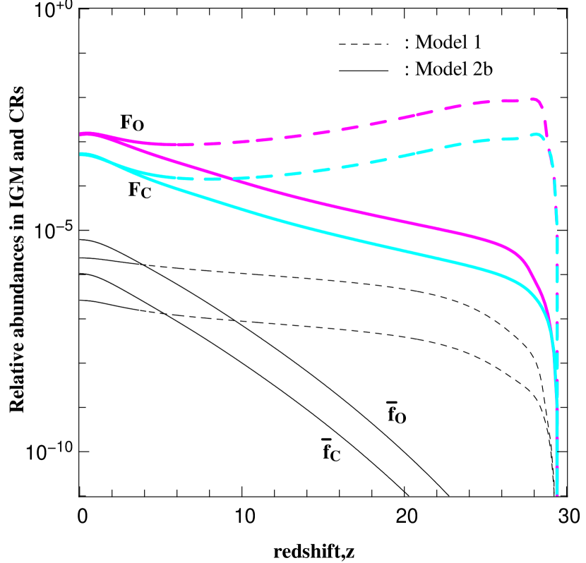
Figure 1.— Relative abundances of C and O in CCRs ($F_{i}$: colored, thick lines) and in the IGM ($\bar{f}_{i}$: black, thin lines) for model 2b (solid) and model 1 (dashed). $F_{i}$ and $\bar{f}_{i}$ are defined in Eqs. (4) and (5).

2.2. Cosmic Ray escape efficiency

In RVOI and RVOII, the efficiency of secondary CR escape from the ISM of early galactic structures (hereafter simply “galaxies”) into the IGM was always assumed to be high. However, as shown in RVOII, the effects of CR heating of the IGM, required a certain degree of confinement of CR propagation and ${}^{6}{\rm Li}$ production to regions that will develop into the warm-hot IGM. Here we present a physical justification of these assumptions.

In accordance with Daigne et al. (2006), we can evaluate the mass $\bar{M}(z)$ of a typical galaxy at redshift $z$ as the mass-weighted average over the Press-Schechter mass function of collapsed dark matter halos $f_{PS}(M,z)$,

$$\bar{M}(z)=\int_{M_{\min}}^{\infty}dMM^{2}f_{PS}(M,z)/\int_{M_{\min}}^{\infty}dMMf_{PS}(M,z),$$ (6)

where $M_{\min}=10^{7}M_{\sun}$. The average ISM density and radius of the galaxy can be estimated respectively as

$$\rho_{\rm ISM}(z)=(\Omega_{b}/\Omega_{m})\Delta_{c}(z)\rho_{c}(z)$$ (7)

and

$$R(z)=(3\bar{M}(z)/4\pi\rho_{c}(z)\Delta_{c}(z))^{1/3},$$ (8)

where $\rho_{c}(z)$ is the critical density of the universe at $z$ and $\Delta_{c}(z)$ is the density contrast of halos virializing at $z$ (e.g. Barkana & Loeb 2001).

CR escape out of the ISM can be mediated either by diffusion or by advection in a galactic outflow. The CR diffusion coefficient $\kappa$ is governed by magnetic fields within early galaxies and is quite uncertain. Here we follow the plausible physical prescription of Jubelgas et al. (2006) and assume $\kappa(p,z)=3\times 10^{27}{\rm cm^{2}s^{-1}}(p/m_{p}c)^{1/3}(n_{\rm ISM}/{\rm cm^{-3}})^{-1/2}$, where $p$ is the CR momentum. Note that we have normalized to the present-day galactic value at unit ISM number density $n_{\rm ISM}$, and neglected the weak dependence on ISM temperature. The timescale for diffusive escape is

$$\tau_{\rm diff}(p,z)=R(z)^{2}/4\kappa(p,z).$$ (9)

Alternatively, CRs may escape by being advected in supernova-driven outflows of ISM gas into the IGM. The timescale for advective escape is simply

$$\tau_{\rm adv}(z)=R(z)/v_{\rm esc}(z),$$ (10)

where $v_{\rm esc}(z)$ can be evaluated as in Daigne et al. (2006).

Ionization losses within the ISM may deplete LiBeB-producing, low energy CRs before they manage to escape. The ionization loss timescale for a CR particle of velocity $\beta c$, charge $Z$ and mass $Am_{p}$ in a medium of neutral H is

$$\tau_{\rm ion}(\beta,z) = (Am_{p}m_{e}c^{3}/4\pi Z^{2}e^{4})\beta(\gamma-1)$$

$$\times[\ln(2m_{e}c^{2}\gamma^{2}\beta^{2}/I_{\rm H})-\beta^{2}]^{-1}n_{\rm ISM}^{-1},$$

where $\gamma=(1-\beta^{2})^{-1/2}$ is the particle Lorentz factor and $I_{\rm H}=13.6$ eV is the H ionization potential (e.g. Longair 1992).

\begin{picture}(9.0,9.0)\centerline{\hbox{\psfig{width=433.62pt}}} \end{picture}

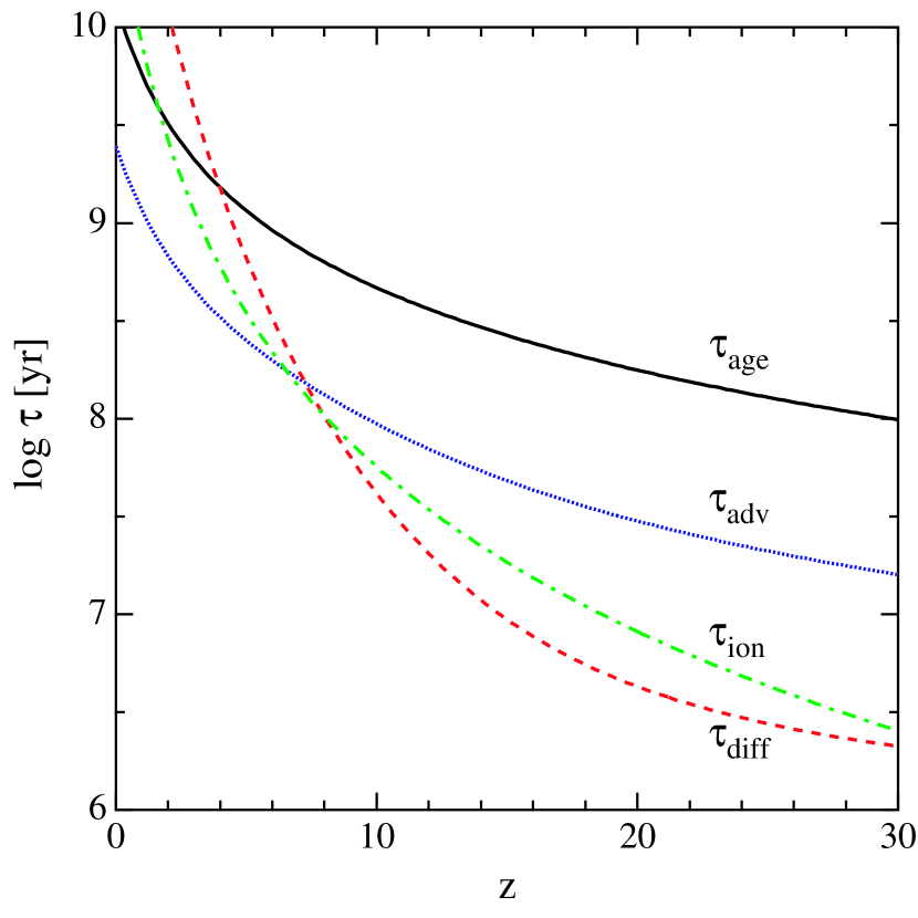
Figure 2.— Timescales for CR escape from typical galaxies into the IGM due to advection $\tau_{\rm adv}$ (dotted, blue) and diffusion $\tau_{\rm diff}$ (dashed, red), and for ionization losses within the ISM $\tau_{\rm ion}$ (dot-dashed, green), for $\alpha$ particles of energy 30 MeV/nucleon, compared with the age of the universe $\tau_{\rm age}$ (solid, black).

In Fig. 2, $\tau_{\rm adv}$, $\tau_{\rm diff}$ and $\tau_{\rm ion}$, the latter two for $\alpha$ particles of kinetic energy 30 MeV/nucleon, as functions of $z$ are compared with the age of the universe $\tau_{\rm age}$, a rough measure of the available time at $z$. We can see that the timescales for CR escape out of the ISM by either diffusion or advection are always much shorter than $\tau_{\rm age}$ at all $z$, with diffusion dominating over advection above $z\sim 7$. This justifies the assumption of RVO2 regarding efficient CR escape into the IGM. However, we see that in some cases ionization losses in the ISM can become important on the escape timescales, and such effects should be included in future, more detailed studies.

While the timescales for advection and diffusion indicate that CRs eventually escape to the IGM, it is important to consider the spallation timescales to determine whether there are any potential effects on the CR spectrum. A simple estimate of the spallation timescale, $\tau_{\rm spal}=[n_{\rm ISM}\beta c\sigma_{\rm tot}]^{-1}$, shows that spallation indeed occurs on timescales shorter than those associated with escape. Noting that the total destruction cross-section is roughly constant above a few hundred MeV and using $\sigma_{\rm tot}^{\rm H}\sim$ 40 mb, $\sigma_{\rm tot}^{\rm He}\sim$ 80 mb, and $\sigma_{\rm tot}^{\rm C}\sim$300 mb, one finds time scales on the order $\tau_{\rm spal}\lesssim 10^{6}$ yrs. This implies that within structures and certainly within volumes associated with the warm-hot IGM, we expect the effects of confinement to play a role and hence allows us to assume a spectrum with a propagated slope of $\gamma=-3$ for p’s and $\alpha$’s and a flattened spectrum of the form given in Eq. (3) for CNO.

We note that the above estimate of $\rho_{\rm ISM}$ should become increasingly inappropriate at lower $z$ when the total halo mass approaches Milky Way scales and the gas within them collapses to a thin disk via efficient radiative cooling. Then the ISM will have a much higher density within a small disk scale height, and much lower density for the remaining halo volume. The CR diffusion time out of the disk should be less than $\tau_{\rm diff}$ at low $z$ as evidenced by the known CR escape time out of the current galactic disk ($\sim 10^{7}$ yr for GeV CRs), and that out of the halo into the IGM should also be less by virtue of the low gas density in the halo.

2.3. Low energy component and neutrino spallation

In the past, it has been shown that, besides standard CRs, there is a need for an additional source of LiBeB in the structures for at least two reasons: standard CRs do not reproduce $(i)$ the meteoritic ¹¹B/¹⁰B isotopic ratio and $(ii)$ the linear (rather than quadratic) proportionality between Be (and B) and Fe in the halo phase. These two constraints can be satisfied taking into account two additional sources of LiBeB (Vangioni-Flam et al., 2000) : $(i)$ the neutrino spallation in the He and C shells of SN, which synthesizes ⁷Li and ¹¹B and $(ii)$ the break-up of low energy nuclei injected in molecular clouds which produces all LiBeB isotopes.

Those additional processes as well as their nucleosynthesis products take place in the structure during SN explosion. They are computed according to Olive et al. (1994); Cassé, Lehoucq & Vangioni-Flam (1995); Vangioni-Flam et al. (1996). The subsequent enrichment of the IGM is due to the global outflow as computed by Daigne et al. (2006).

3. Results

For all elements $X$, primordial abundances are assumed at the initial redshift $z=30$ of the model. The production of $X$ by CCR interactions in the IGM is integrated down to $z=0$. In addition, the abundance of each element is affected by outflows: these contributions are shown separately in the figures. The calculation for D, Be and B production follows closely that of the ⁶Li, as given, for example, in RVOI. The full calculation is then compared to a simplified calculation (Eq. A7 and values gathered in Tab. 1; App. A). Note that throughout the paper, $E$ denotes the kinetic energy per nucleon.

3.1. Lithium

The abundance of lithium in the IGM increases with decreasing redshift due to the interaction of CR $\alpha$’s with He at rest in the IGM (the cross section peaks at 10 MeV/n). Since the total energy in CRs is proportional to $\epsilon_{\rm CR}$, the amount of lithium produced depends on both $\gamma$ and $\epsilon_{\rm CR}$ and of course on the assumed model for star formation. Note that lithium is also produced through CNO interactions with H and He at rest. These are taken into account in the calculation, but the contribution to the total abundance of Li is always subdominant in this context (§2.1.1).

We have constrained $\epsilon_{\rm CR}$ to insure a PIE of ${}^{6}{\rm Li}$ with abundance ${}^{6}{\rm Li}$/H $=10^{-11.2}$ at $z=3$. The results for model 1 and model 2b are shown in Fig. 3 (dashed and solid lines respectively). Model 1 was already discussed in RVOII and it was determined there that $\epsilon_{\rm CR}\simeq 0.15$ was necessary to produce the requisite amount of ${}^{6}{\rm Li}$. In model 2b, however, PopIII stars terminate as black holes, with no assumed production of cosmic rays. Thus, the lithium production is delayed and a higher efficiency is required, $\epsilon_{\rm CR}\simeq 0.5$. Such a high value is consistent with those found in diffusive shock acceleration models (Berezhko & Völk, 1997; Berezhko & Ellison, 1999; Berezhko & Völk, 2000, 2006; Blasi, Gabici & Vannoni, 2005; Ellison & Cassam-Chenaï, 2005; Kang & Jones, 2006; Ellison et al., 2007), as confirmed by recent comparison with observations of supernova remnants (e.g. Berezhko & Völk, 2004; Warren et al., 2005).

The additional lithium due to outflows from the inner regions (as discussed in Section 2.3) is small (dotted lines in Fig. 3) compared to the ${}^{6}{\rm Li}$ production by CR interactions with the IGM. Also shown in Fig. 3 is the evolution of ${}^{7}{\rm Li}$ assuming the initial primordial value of ${}^{7}{\rm Li}$/H = $4.15\times 10^{-10}$ determined by BBN at the WMAP value for the baryon density (Coc et al., 2004): as already emphasized in RVOI, the additional CCR production of ${}^{7}{\rm Li}$ is negligible compared to that produced by BBN.

\begin{picture}(9.0,9.0)\centerline{\hbox{\psfig{width=433.62pt}}} \end{picture}

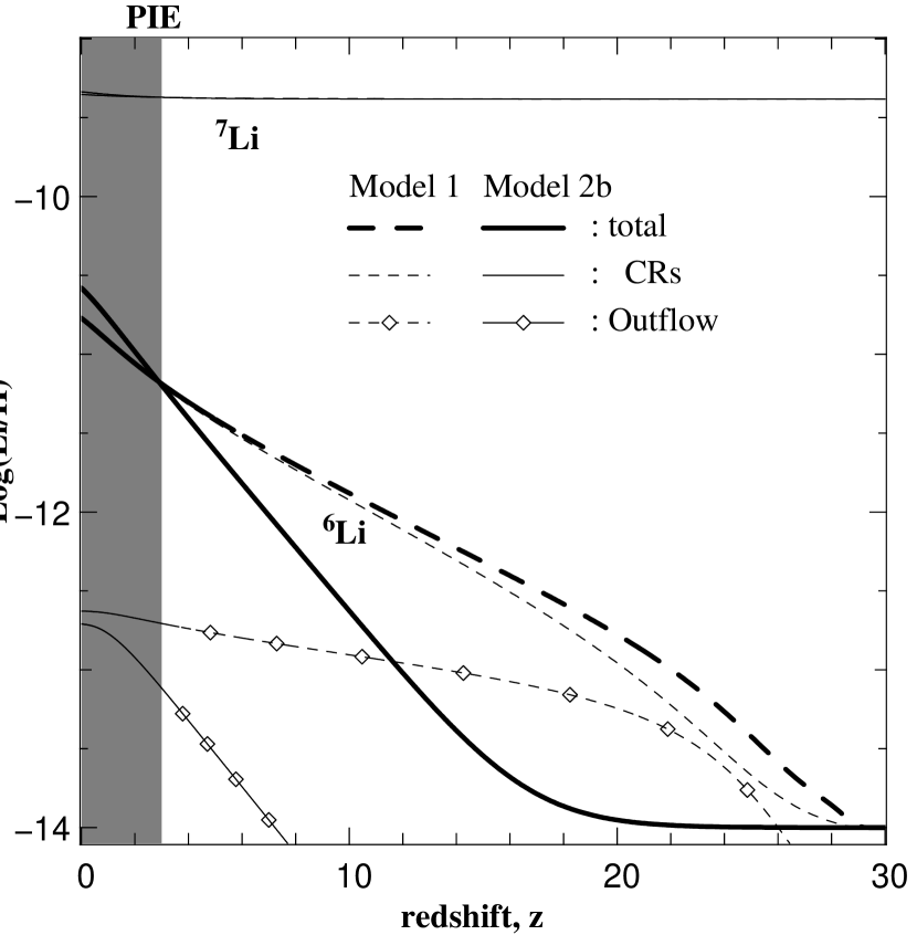
Figure 3.— Nucleosynthesis of both isotopes of lithium through the interactions of secondary CCR $\alpha$ particles impinging on He in the IGM including the effects of outflow. For a given star formation history (taken here to be model 1 and model 2b of Daigne et al. 2006) and a slope of the CCR energy spectrum ($\gamma=3$), the acceleration efficiency of the CCRs is set to obtain a PIE which equals the observed plateau ⁶Li/H=$10^{-11.2}$ at $z=3$: this leads to $\epsilon_{\rm CR}=0.15$ for model 1 and $\epsilon_{\rm CR}=0.5$ for model 2b. The individual contributions to the lithium abundance due to CR’s and outflows from the ISM are shown by the thin curves as indicated in the legend.

3.2. Deuterium

There are two main production reactions for deuterium, namely pH and pHe. For the simplified calculation, assuming $\gamma=3$ and the two extreme cases for $I(\gamma,p_{1},p_{2})$, as given in Eq. (A6), we obtain

$$\left[\frac{{\rm D}_{\rm pH}}{\mbox{${}^{6}$Li}}\right]\approx 5\quad{\rm and}\quad\left[\frac{{\rm D}_{\rm pHe}}{\mbox{${}^{6}$Li}}\right]\approx 50\,.$$ (12)

This makes a total contribution of about D/${}^{6}{\rm Li}$ $\sim 100$ coming from pH, pHe and the numerically similar reverse process $\alpha$p, independent of the redshift. This is consistent with the constant value of 70 derived in the exact calculation. Thus, the additional production of deuterium by CCRs at $z=3$ is about $3.1\times 10^{-10}$ and is therefore well below the observed abundance D/H$\,\sim\,2\times 10^{-5}$ (O’Meara et al., 2006).

3.3. BeB

Beryllium and boron are produced via spallation interaction between protons or $\alpha$’s in CRs and CNO elements in the IGM. The reverse reactions, which correspond to CNO CRs spalling on H and He of the IGM, is in fact dominant. This can be understood as the metallicity in the ISM (where CRs originate) is always larger than that in the IGM. In contrast to the galactic disc, the heavy nuclei component of CCRs becomes important due to the metal deficiency of the IGM. Qualitatively, the ratio of the forward to reverse processes is given by

$$\left[\frac{({\rm BeB})_{\rm pO}}{({\rm BeB})_{\rm OH}}\right]=\frac{\bar{f}_{\rm O}}{F_{\rm O}}=\frac{[{\rm O/H}]_{\rm IGM}}{\eta_{\rm O}[{\rm O/H}]_{\rm ISM}}\;,$$ (13)

where $\bar{f}$, $F$ and $\eta$ are defined in Eq. (4) and Eq. (5). From the calculated abundances of Daigne et al. (2006), the metallicity ratio between the IGM and CRs is $\lesssim 10^{-2}$ (see eg. Fig. 1), so that, the forward process is $\sim 10^{-3}$ smaller than the reverse. For the reverse process, Eq. (A7) does not apply in principle, since $F_{i}$ no longer factors out of the $z$ integrand. However, in the CRs, $F_{C}\lesssim 10^{-4}$ and $F_{O}\lesssim 10^{-3}$ (see Fig. 1). An upper limit to the production of ⁹Be, would then be, for $\gamma_{\rm O}=3$, ${{}^{9}{\rm Be}_{\rm OH}}/{\mbox{${}^{6}$Li}}\approx 0.3$. This compares well with the full calculation (upper solid line in Fig. 4). The leading contribution of the reverse process is confirmed in Fig. 4 for the full calculation in model 2b (upper solid line compared to dashed line) ; the same is also true for model 1. The same reasoning holds for reactions involving C, N. The dominant channel is actually O+H. Nevertheless, all nuclei are accounted for in the full calculation below. As one can see in Fig. 4, adopting the spectral break, i.e. $\gamma_{\rm O}=1.5$ as described in Section 2.1.1, decreases the contribution of the reverse process and as a result lowers the Be abundance as shown by the thick solid curve compared to the upper thin curve with $\gamma_{\rm O}=3$.

\begin{picture}(9.0,10.0)\centerline{\hbox{\psfig{width=433.62pt}}} \end{picture}

Figure 4.— Beryllium production by the interaction of CCRs and the IGM for model 2b. The direct reaction p+O (dashed line) is negligible compared to the reverse reaction O+H (solid thick line). The upper thin solid curve displays the ${}^{9}{\rm Be}$ production as a function of redshift assuming an O spectrum with $\gamma_{\rm O}$ = 3 as for p and He at low energy The thin dashed curve assumes $\gamma_{\rm p,He}$ = 3. The thick solid curve is based on Eq. (3) and assumes $\gamma_{\rm O}$ = 1.5 at low energy.

\begin{picture}(9.0,9.0)\centerline{\hbox{\psfig{width=433.62pt}}} \end{picture}

Figure 5.— Nucleosynthesis of beryllium and boron through the interaction of secondary CR p’s, $\alpha$’s and (CNO) impinging on CNO (H and He) in the IGM including the effects of outflow. The evolution of the abundance of ⁹Be and ^10,11B is displayed as a function of redshift for models 1 and 2b. The individual contributions to the beryllium abundance due to CR’s and outflows from the ISM are shown by the thin curves as indicated in the legend.

\begin{picture}(9.0,9.0)\centerline{\hbox{\psfig{width=433.62pt}}} \end{picture}

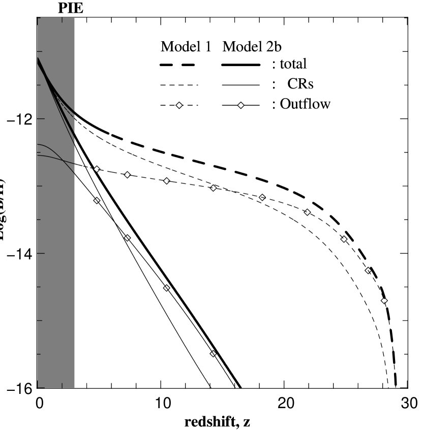
Figure 6.— As in Fig. 5, for boron.

The results from the full calculation of the BeB abundances for both models 1 and 2b are given in Figs. (5)-(6). Note once again that BeB production in model 2b is delayed due to the lack of metal enrichment in the ISM from the massive mode in this model. At $z=3$, we find ${}^{9}{\rm Be}$/H$=10^{-12.9}$ in model 1 (upper panel) and ${}^{9}{\rm Be}$/H$=10^{-13.3}$ in model 2b (lower panel). This is compatible with the observed abundance at the lowest metallicity, [Fe/H]$=-3.3$, ⁹Be/H$\sim\,10^{-13}$ in G64-12 (Primas et al., 2000a). For boron, we find B/H $=10^{-11.9}$ in model 1 and and B/H $=10^{-12.25}$ in model 2b. These values are somewhat below the observed boron abundance at low metallicity B/H$\sim\ 10^{-11.3}$ at [Fe/H]$=-3.0$ in BD -13 3442 (Primas et al., 2000b) though B/H is as low as $10^{-12}$ at [Fe/H]$=-2.9$ in BD -23 3130 (García-López et al., 1998). Note however, that unlike beryllium abundances, the boron abundances in particular are very sensitive to the assumed effective temperature. The abundances quoted above were determined using temperatures based on the IRFM (Alonso, Arribas, & Martinez-Roger, 1996). The boron abundance in BD -13 3442 would be $10^{-10.7}$ (Fields et al., 2005) had we adopted the temperature derived by Meléndez & Ramírez (2004). Of course Li also scales with temperature and at higher effective temperatures, the level of the ${}^{6}{\rm Li}$ plateau would be raised forcing one to large CR efficiencies.

Our results can be cast in terms of abundance ratios of ${}^{9}{\rm Be}$/${}^{6}{\rm Li}$ and B/${}^{6}{\rm Li}$

$$\left[\frac{{}^{9}{\rm Be}}{\mbox{${}^{6}$Li}}\right]\approx 0.020\qquad\left[\frac{\rm B}{\mbox{${}^{6}$Li}}\right]\approx 0.20\;,$$ (14)

for model 1 and

$$\left[\frac{{}^{9}{\rm Be}}{\mbox{${}^{6}$Li}}\right]\approx 0.008\qquad\left[\frac{\rm B}{\mbox{${}^{6}$Li}}\right]\approx 0.09\;.$$ (15)

for model 2b. These predicted ratios are independent of the efficiency $\epsilon_{\rm CR}$ and can be compared to the few examples where observational determinations of ${}^{6}{\rm Li}$ and Be exist in the same star. Restricting our attention to only those stars with [Fe/H] ¡ - 2.6, we have Be abundance measurements in two stars, G64-12 (Primas et al., 2000a) and LP 815-43 (Primas et al., 2000b) for which there are reliable ${}^{6}{\rm Li}$/${}^{7}{\rm Li}$ determinations (Asplund et al., 2006; Inoue et al., 2005). When corrected for stellar temperature differences, we find ${}^{9}{\rm Be}$/${}^{6}{\rm Li}$ = $0.005\pm 0.003$ for G64-12 and = $0.011\pm 0.007$ for LP 815-43. Unfortunately there are no very low metallicity stars with both ${}^{6}{\rm Li}$ and B abundance measurements.

The predicted PIE at $z=3$ for both elements is of the same order as the abundances observed at the lowest metallicity. Thus we expect a plateau in both Be and B at low metallicity similar to that found for ${}^{6}{\rm Li}$. Indeed, when the Be abundance in G64-12 was first reported (Primas et al., 2000a), the authors claimed evidence for a flattening of the observed Be evolutionary trend at low metallicity. It will be interesting if future determinations of Be at low metallicity confirm the existence of a Be plateau.

We have also computed the production of BeB through LEC nucleosynthesis and neutrino spallation via outflow to the IGM. In all cases, the abundance produced by these processes is less at small redshift, though the abundance of ${}^{11}{\rm B}$ produced by the $\nu$-process is not negligible at higher redshift. These results are displayed by the thin lines in Figs. (5)-(6).

3.4. Pionic production of gamma-rays

The interaction of the CCRs with the IGM also produces gamma-rays. Our calculation closely follows that given in Pavlidou & Fields (2002). Assuming isotropic production, the extragalactic differential flux of $\gamma$-rays at Earth in the flat $\Lambda$CDM cosmology is

$$\frac{dF_{\gamma}}{dE}=\frac{c}{4\pi H_{0}}\int_{0}^{\infty}dz\;\frac{q_{\gamma}(z,E^{\prime}=(1+z)E))}{(1+z)^{3}\,\sqrt{\Omega_{\Lambda}+(1+z)^{3}\Omega_{\rm M}}}\;.$$ (16)

The $\gamma$-ray source function $q_{\gamma}(z,E^{\prime})$ is calculated using the simplified analytic formula of Pfrommer & Ensslin (2004):

$$q_{\gamma}(z,E^{\prime}) \approx \sigma_{\rm pp}\phi_{\rm p}(E^{\prime})n_{\rm IGM}(z)\zeta^{2-\alpha}$$ (17)

$$\times \frac{4m_{\pi^{0}}}{3\alpha_{\gamma}}\times\left[\left(\frac{2E^{\prime}_{\gamma}}{m_{\pi^{0}}}\right)^{\delta}_{\gamma}+\left(\frac{2E^{\prime}_{\gamma}}{m_{\pi^{0}}}\right)^{-\delta_{\gamma}}\right]^{-\alpha_{\gamma}/\delta_{\gamma}}$$

with $\zeta=2$, $\delta_{\gamma}=0.14\alpha_{\gamma}^{-1.6}+0.44$ and $\sigma_{\rm pp}=32\times(0.96+e^{4.4-2.4\alpha_{\gamma}})$ mb. The same input fluxes and IGM densities are taken as for the D and LiBeB calculations. Fig. 7 shows that the total $\gamma$-ray flux produced by CCRs is negligible compared to the observed EGRB.

\begin{picture}(9.0,9.0)\centerline{\hbox{\psfig{width=433.62pt}}} \end{picture}

Figure 7.— Energy spectrum (E²I versus energy in GeV) of photons produced by pion decay in the IGM. The models are well below the observed EGBR data (Strong, Moskalenko & Ptuskin, 2007).

4. Discussion and conclusions

Our initial motivation to study CCRs at high redshift was to find a physical origin for the anomalously high abundance of ⁶Li observed in metal poor halo stars. A cosmic history for structure formation that reproduces standard observations (Daigne et al., 2006) provides enough energy in SN to produce a ⁶Li plateau at the level of $\log[\mbox{${}^{6}$Li}/{\rm H}]\approx-11.2$ via $\alpha+\alpha$ interactions of CCRs with the IGM. Note that the ⁶Li produced by outflows (via neutrino spallation and LEC) is negligible.

In this paper, we considered two models of star formation histories differing by their Pop III stars. The massive component of model 1 ($40-100M_{\odot}$) injects a lot of energy in CCRs so that the necessary fraction $\epsilon_{\rm CR}$ is low ($\sim 0.15$). On the other hand, the stars associated with the massive component of model 2b ($260-500M_{\odot}$) are assumed to collapse into black holes without injecting, a priori, any energy in CCRs. Consequently, the fraction $\epsilon_{\rm CR}$ associated with SN in the normal mode must be higher ($\sim 0.5$). This figure would be reduced if super massive stars produce CRs.

We confirm, as in RVOII, that the ⁷Li primordial abundance always dominates any additional production by CCRs. The same conclusion holds for deuterium. Similarly, the observed EGBR is much larger than the intensity of photons produced by the decay of pions produced by CCR proton collisions.

In the same cosmological context, we explored the production of other light elements (BeB). To that end, it is necessary to track the abundances of metals (CNO) in the ISM and IGM. We have shown that the reverse process (i.e. CNO CCRs on H and He IGM gas) is the dominant channel to synthesize BeB. This is in contrast to the production of BeB in the galactic disk, where the reverse process contributes roughly 20% (Meneguzzi, Audouze & Reeves, 1971). This is easily understood as the metal enrichment in CCRs is inherited from structure abundances, which are far higher than those in the IGM. Note that we also checked that the neutrino spallation and LEC processes are negligible in the IGM BeB budget at the time of the galactic formation, i.e. $z\sim 3$. In all models considered, we have shown that BeB synthesized at $z\sim 3$ is at the level of the observed abundances in the lowest metallicity stars. This is the first theoretical indication of a plateau for these elements which does not resort to exotic models of BBN.

Note that these results have been obtained with several assumptions about the CCR spectra. To some extent, our modeling, be it for light elements (pHe) or metals (CNO), is limited. Indeed, two fundamental ingredients for the calculation are i) the low energy form of the source spectra for protons and ii) the propagated fluxes to plug in the IGM. The first item is crucial for determining the acceleration efficiency $\epsilon_{\rm CR}$. For example, changing $\gamma\approx 3$ to $\gamma\approx 2$—hence taking a more conventional spectral index for the sources—would lead to an unphysical value of $\epsilon_{\rm CR}>1$. However, we expect that propagation effects on scales of order the warm-hot IGM would lead to a steeper spectrum (i.e. $\gamma=3$ for p’s and $\alpha$’s) and a flatting of the CNO spectrum of the form we have assumed here. The second item involves several issues that are intimately connected: the details of CR escape and confinement between the structures, the warm-hot IGM and cooler IGM is related to whether or not the propagated spectrum displays a spectral index close to the standard source index ($\gamma\approx 2$) or closer to a diffused spectrum ($\gamma\approx 3$) and, more importantly, how this evolves with $z$. Without some degree of confinement on the scale of the warm-hot IGM, we would be forced to take the same spectrum for p, He and CNO nuclei—as would be more natural for a 100% escape to the IGM, and this would lead to an overproduction of ⁹Be. Our simple estimate of the spallation timescale within structures indicates that confinement is indeed playing a role and changes to the CR source spectrum will occur.

All of these elements clearly call for a more coherent and refined calculation. As just outlined, one issue concerns the description of CR propagation in realistic structures, evolving with redshift, which also allows for differentiated production in situ and outside structures. Another important issue is the possibility for heterogeneity in metallicities at a given time (e.g. Salvadori, Schneider & Ferrara 2006), that cannot be handled in the homogeneous paradigm developed in Daigne et al. (2006). This question could be addressed when ⁶Li and ⁹Be are observed simultaneously. Finally, we note that B can be observed directly in high redshift objects, as achieved for a damped Ly$\alpha$ system at $z=2.6$ (Prochaska et al., 2003). Observations at even higher $z$ may be possible through absorption lines in gamma-rays bursts (J. Prochaska, private communication), which should provide very valuable constraints on early LiBeB production scenarios.

Appendix A Simplified calculation for D-Be-B

The calculation for D, Be and B production follows closely that of the ⁶Li, as given, for example, in RVOI. In this appendix, we estimate the relative efficiency of various channels as well as the relative efficiency of the D, Be and B production with respect to the ⁶Li production. In some cases, the latter is independent of $z$. Below, $E$ denotes the kinetic energy per nucleon.

The abundance of the element $X$ relative to $H$ is given by

$$\left[\frac{X}{H}\right]_{z_{0}}=\sum_{i=CR}\;\sum_{j=IGM}\int_{z_{0}}^{\infty}\int_{E_{\rm cut}}^{\infty}\bar{f}_{j}\;\sigma_{ij}^{X}(E_{\rm p})\;F_{i}\;\Phi_{\rm p}(E_{\rm p},z)\;dE_{\rm p}\left|\frac{dt}{dz}\right|dz\;,$$ (A1)

where $\Phi_{\rm p}(E_{\rm p},z)$ is the accumulated CR proton flux in the IGM (in proper units), $\sigma_{ij}^{X}(E_{\rm p})$ is the production cross section of $X$ in the reaction $(i+j)$ and $f_{i}$ and $F_{i}$ are defined in Eqs. (4) and (5). Note that ⁶Li is only produced by CR $\alpha$’s with energy four times the final lithium energy. As a consequence, the above formula also applies to [⁶Li/H], but an extra factor $1/4$ must be added. Two simplifications are made:

• All cross sections $\sigma_{ij}^{X}(E)$ are approximated as a constant in the range $E_{1}-E_{2}$ and zero elsewhere, i.e.

  $$\sigma_{ij}^{X}(E)=\sigma_{ij}^{X}\times\Theta(E-E_{1})\Theta(E_{2}-E)\;.$$ (A2)

  The values of the cross sections for the main processes are given in Tab. 1.

• $\Phi_{\rm p}(E_{\rm p},z)$ is assumed to keep the same power law dependence $\gamma$ as the source spectrum at each $z$, so that it can be rewritten as

  $$\Phi_{\rm p}(E_{\rm p},z)=N_{0}(z)\Phi_{\rm p}(E_{\rm p})\;.$$ (A3)

$i+j\rightarrow X$	$\sigma_{ij}^{X}$ (mb)	$E_{1}$ (GeV/n)	$E_{2}$ (GeV/n)
$\alpha\!\/$ + He $\rightarrow\mbox{${}^{6}$Li}$	20	0.01	0.02
p + H   $\rightarrow$   D	1	0.4	0.8
p + He $\rightarrow$   D	12	0.05	$\infty$
p + C   $\rightarrow\,^{9}$Be	6	1.0	$\infty$
p + O   $\rightarrow\,^{9}$Be	5	0.05	$\infty$
p + C   $\rightarrow$   B	90	0.015	$\infty$
p + O   $\rightarrow$   B	50	0.04	$\infty$

Table 1Simplified description of cross sections used in the approximate calculation

If $j={\rm H,~{}He}$, $\bar{f}_{j}$ and $F_{i}$ are constants that factor out of the $z$ integrand:

$$\left[\frac{X}{H}\right]_{z_{0}}=\sum_{i=CR}\;\sum_{j=IGM}\bar{f}_{j}\;F_{i}\;\sigma_{ij}^{X}\;I\left(\nu,p_{1}(E_{1}),p_{2}(E_{2})\right)\int_{z_{0}}^{\infty}N_{0}(z)\left|\frac{dt}{dz}\right|dz\;,$$ (A4)

where

$$I(\gamma,p_{1}(E_{1}),p_{2}(E_{2}))\equiv\int_{p_{1}}^{p_{2}}\frac{p^{-\gamma+1}}{\sqrt{p^{2}+m_{p}^{2}}}dp\;,$$ (A5)

and where $p(E)$ is the CR proton momentum for a given kinetic energy per nucleon E. This function can be integrated as a hyperbolic function, but for the purpose of a simplified calculation, it is good enough to consider the two limits, that apply either when the production is at very low energy (e.g. for ⁶Li), or at GeV/n energies:

$$I_{p\ll m_{p}}\approx\left[\frac{p^{-\gamma+2}}{2-\gamma}\right]_{p_{1}}^{p_{2}}\quad{\rm and}\quad I_{\beta\sim 1}\approx\left[\frac{p^{-\gamma+1}}{1-\gamma}\right]_{p_{1}}^{p_{2}}\;.$$ (A6)

We shall now write a simplified expression for the comparison of the production of $X$ with respect to ⁶Li. The integration over $z$ cancels out, and this results in

$$\left[\frac{X}{\mbox{${}^{6}$Li}}\right]=\frac{\displaystyle\sum_{i=CR}\;\sum_{j=IGM}\bar{f}_{j}\;F_{i}\;\,\sigma_{ij}^{X}\,\;\,I^{X}_{i}}{\displaystyle\bar{f}_{He}\;(F_{He}/4)\,\;\,\sigma_{\alpha\alpha}^{{}^{6}Li}\,\;\,I_{\alpha}^{{}^{6}Li}}\;,$$ (A7)

where we wrote $I(\gamma,p_{1}(E^{i}_{1}),p_{2}(E^{i}_{2}))\equiv I^{X}_{i}$ for short.

References

- Alonso, Arribas, & Martinez-Roger (1996) Alonso, A., Arribas, S., & Martinez-Roger, C. 1996, A&AS 117, 227
- Asplund et al. (2006) Asplund, M., Lambert, D. L., Nissen, P. L., Primas, F. & Smith, V. V. 2006, ApJ 644, 229
- Barkana et al. (2001) Barkana, R. & Loeb, A. 2001, Phys. Rep. 349, 125
- Berezhko & Ellison (1999) Berezhko, E. G. & Ellison, D. C. 1999, ApJ 526, 385
- Berezhko & Völk (1997) Berezhko, E. G. & Völk, H. J. 1997, Astropart. Phys. 7, 183
- Berezhko & Völk (2000) Berezhko, E. G. & Völk, H. J. 2000, A&A 357, 283
- Berezhko & Völk (2004) Berezhko, E. G. & Völk, H. J. 2004, ApJ 419, 27
- Berezhko & Völk (2006) Berezhko, E. G. & Völk, H. J. 2006, A&A 451, 981
- Blandford & Eichler (1987) Blandford, R., Eichler, D. 1987, Phys. Rep. 154, 1
- Blasi, Gabici & Vannoni (2005) Blasi, P., Gabici, S., Vannoni, G. 2005, MNRAS 361, 907
- Bonifacio et al. (2007) Bonifacio, P., et al. 2007, A&A, 462, 851
- Cassé, Lehoucq & Vangioni-Flam (1995) Cassé, M., Lehoucq, R. & Vangioni-Flam, E. 1995, Nature 373, 38
- Cayrel et al. (1999) Cayrel, R., Spite M., Spite F., Vangioni-Flam, E., Cassé, M. & Audouze, J. 1999, A&A 343, 923
- Coc et al. (2004) Coc, A., Vangioni-Flam, E., Descouvemont, P., Adahchour, A., & Angulo, C. 2004, ApJ 600, 544
- Cuoco et al. (2004) Cuoco, A., Iocco, I., Mangano, G., Pisanti, O., & Serpico, P. D. 2004, Int. Mod. Phys. A19, 4431
- Cyburt et al. (2006) Cyburt, R. H., Ellis, J., Fields, B. D., Olive, K. A., & Spanos, V. C. 2006, JCAP 11, 14
- Cyburt, Fields, & Olive (2001) Cyburt, R. H., Fields, B. D., & Olive, K. A. 2001, New Astron. 6, 215
- Cyburt, Fields, & Olive (2002) Cyburt, R. H., Fields, B. D., & Olive, K. A. 2002, Astropart. Phys. 17, 87
- Cyburt, Fields, & Olive (2003) Cyburt, R. H., Fields, B. D., & Olive, K. A. 2003, Phys. Lett. B 567, 227
- Cyburt (2004) Cyburt, R. H., 2004, Phys. Rev. D 70, 023505
- Daigne et al. (2006) Daigne, F., Olive, K. A., Silk, J., Stoehr, F., & Vangioni-Flam, E. 2006, ApJ 647, 773
- Drury (1983) Drury, L. O’C. 1983, Rep. Prog. Phys. 46, 973
- Ellison, Drury & Meyer (1997) Ellison, D. C., Drury, L. O., & Meyer, J.-P. 1997, ApJ 487, 197
- Ellison & Cassam-Chenaï (2005) Ellison, D. C. & Cassam-Chenaï, G. 2005, ApJ 632, 920
- Ellison et al. (2007) Ellison, D. C., Patnaude, D. J., Slane, P., Blasi, P., Gabici, S. 2007, ApJ 661, 879
- Fields & Olive (1999) Fields, B. D., & Olive, K. A. 1999, New. Astron. 4, 255
- Fields et al. (2005) Fields, B. D., Olive, K. A., & Vangioni-Flam, E. 2005, ApJ 623, 1083
- Fields & Prodanović (2005) Fields, B. D., & Prodanović, T. 2005, ApJ 623, 877
- Heger et al. (2003) Heger, A., Fryer, C.L., Woosley, S.E., Langer, N., & Hartmann, D.H. 2003, ApJ 591, 288
- Heger et al. (2005) Heger, A., Kolbe, E., Haxton, W. C., Langanke, K., Martínez-Pinedo, G., & Woosley, S. E. 2005, Physics Letters B 606, 258
- Hobbs & Thorburn (1994) Hobbs, L.M. & Thorburn, J.A. 1994, ApJ 428, L25
- Hobbs & Thorburn (1997) Hobbs, L.M. & Thorburn, J.A. 1997, ApJ 491, 772
- García-López et al. (1998) García-López, R.J., et al. 1998, ApJ 500, 241
- Horandel (2007) Hörandel, J., 2007, 36th COSPAR Scientific Assembly Beijing, China (astro-ph/0702370)
- Inoue et al. (2005) Inoue, S., 2005, IAU Symposium 228, Edts V. Hill, P. Francois, F. Primas, Cambridge Un. Press, p. 59.
- Jedamzik et al. (2005) Jedamzik, K., Choi, K. Y., Roszkowski, L., & Ruiz de Austri, R. 2006, JCAP 07, 007
- Jones (1994) Jones, F. C. 1994, ApJS90, 561
- Jubelgas et al. (2006) Jubelgas, M., Springel, V., Ensslin, T. A. & Pfrommer, C., A&A submitted (astro-ph/0603485)
- Kang & Jones (2006) Kang, H., Jones, T. W. 2006, Astropart. Phys. 25, 246
- Kawasaki et al. (2005) Kawasaki, M., Kohri, K., & Moroi, T. 2005, Phys. Rev. D 71, 083502
- Kusakabe, Kajino & Mathews (2006) Kusakabe, M., Kajino, T., & Mathews, G.J. 2006, Phys. Rev. D 74, 023526
- Longair (1992) Longair, M. S. 1992, High Energy Astrophysics Vol.1, Cambridge Univ. Press
- Meléndez & Ramírez (2004) Meléndez, J. & Ramírez, I. 2004, ApJ 615, 33
- Meneguzzi, Audouze & Reeves (1971) Meneguzzi, M., Audouze, J. & Reeves, H. 1971, A&A 15, 337
- Maurin et al. (2004) Maurin, D., Taillet, R., Donato, F., Salati, P., Barrau, A. & Boudoul, G. 2004 (Research Signposts, Recent Research Developments in Astronomy and Astrophys. 2, 193 (astroph/021211)
- Meyer, Drury & Ellison (1997) Meyer, J.-P., Drury, L. O., & Ellison, D. C. 1998, Space Sci. Rev. 86, 179
- Meyer, Drury & Ellison (1998) Meyer, J.-P., Drury, L. O., & Ellison, D. C. 1997, ApJ 487, 182
- Nakamura et al. (2006) Nakamura, K., Inoue, S., Wanajo, S. & Shigeyama, T. 2006, ApJ 643, L115
- Nissen et al. (2000) Nissen, P. E., Asplund, M., Hill, V. & D’Odorico, S. 2000, A&A 357, L49
- Olive et al. (1994) Olive, K.A., Prantzos, N., Scully, S., & Vangioni-Flam, E., 1994, ApJ 424, 666
- O’Meara et al. (2006) O’Meara, J. M., Burles, S., Prochaska, J. X., Prochter, G. E., Bernstein, R. A., & Burgess, K. M. 2006, ApJ 649, L61
- Pavlidou & Fields (2002) Pavlidou, V., & Fields, B. D. 2002, ApJ 575, L5
- Pospelov (2006) Pospelov, M. 2006, astro-ph/0605215
- Primas et al. (2000a) Primas, F., Asplund, M., Nissen, P.E. & Hill, V. 2000a, A&A 364, L42
- Primas et al. (1999) Primas, F., Duncan, D.K., Peterson, R.C., & Thorburn, J.A. 1999, A&A 343, 545
- Primas et al. (2000b) Primas, F., Molaro, P., Bonifacio, P. & Hill, V. 2000b, A&A 362, 666
- Prochaska et al. (2003) Prochaska, J. X., Howk, J. C. & Wolfe, A. M. 2003, Nature 423, 57
- Rollinde, Vangioni, & Olive (2005) Rollinde, E., Vangioni, E., & Olive, K. 2005, ApJ 627, 666
- Rollinde, Vangioni, & Olive (2006) Rollinde, E., Vangioni, E., & Olive, K. 2006, ApJ 651, 658
- Ryan et al. (2000) Ryan, S. G., Beers, T. C., Olive, K. A., Fields, B. D., & Norris, J. E. 2000, ApJ 530, L57
- Salvadori, Schneider & Ferrara (2006) Salvadori, S., Schneider, R., Ferrara, A. 2006, astro-ph/0611130
- Silk & Schramm (1992) Silk, J. & Schramm, D. N. 1992, ApJ 393, L09
- Smith et al. (1993) Smith, V. V., Lambert, D. L. & Nissen, P. E. 1993, ApJ 408, 262
- Smith, Lambert, & Nissen (1998) Smith, V.V., Lambert, D.L. & Nissen, P.E., 1998, ApJ 506, 405
- Spergel et al. (2007) Spergel, D. N., et al. 2007, ApJS 170, 377
- Spite & Spite (1982) Spite, F. & Spite, M. 1982. A&A 115, 357
- Steigman et al. (1993) Steigman, G., Fields, B.D., Olive, K.A., Schramm, D.N., & Walker, T.P. 1993, ApJ 415, L35
- Strong, Moskalenko & Ptuskin (2007) Strong, A. W., Moskalenko, I. V. & Ptuskin, V. S., 2007, Annu. Rev. Nucl. Part. Sci. 57, 285
- Suzuki & Inoue (2002) Suzuki, T.K., & Inoue, S. 2002, ApJ 573, 168
- Tatischeff & Thibaud (2007) Tatischeff, V. & Thibaud, J. 2007, A&A 469, 265
- Thomas, Schramm, Olive, & Fields (1993) Thomas, D., Schramm, D. N., Olive, K. A., & Fields, B. D. 1993, ApJ 406, 569
- Vangioni-Flam et al. (1996) Vangioni-Flam, E., Cassé, M., Field, B., & Olive, K.A. 1996, ApJ 468, 199
- Vangioni-Flam et al. (1999) Vangioni-Flam, E. et al. 1999, New. Astron. 4, 245
- Vangioni-Flam et al. (2000) Vangioni-Flam, E., Cassé, M. and Audouze, J. 2000, Phys. Rep. 333, 365
- Warren et al. (2005) Warren, J. S., Hughes, J. P., Badenes, C., Ghavamian, P., McKee, C. F., Moffett, D., Plucinsky, P. P., Rakowski, C., Reynoso, E., Slane, P. 2005, ApJ 634, 376
- Woosley et al. (1990) Woosley, S. E., Hartmann, D. H., Hoffman, R. D., & Haxton, W. C. 1990, ApJ 356, 272