Master crossover behavior of parachor correlations for one-component fluids.

Abstract

The master asymptotic behavior of the usual parachor correlations, expressing surface tension $\sigma$ as a power law of the density difference $\rho_{L}-\rho_{V}$ between coexisting liquid and vapor, is analyzed for a series of pure compounds close to their liquid-vapor critical point, using only four critical parameters $\left(\beta_{c}\right)^{-1}$, $\alpha_{c}$, $Z_{c}$ and $Y_{c}$, for each fluid. This is accomplished by the scale dilatation method of the fluid variables where, in addition to the energy unit $\left(\beta_{c}\right)^{-1}$ and the length unit $\alpha_{c}$, the dimensionless numbers $Z_{c}$ and $Y_{c}$ are the characteristic scale factors of the ordering field along the critical isotherm, and the temperature field along the critical isochor, respectively. The scale dilatation method is then formally analogous to the basic system-dependent formulation of the renormalization theory. Accounting for the hyperscaling law $\frac{\delta-1}{\delta+1}=\frac{\eta-2}{2d}$, we show that the Ising-like asymptotic value $\pi_{a}$ of the parachor exponent is unequivocally linked to the critical exponents $\eta$, or $\delta$, by $\frac{\pi_{a}}{d-1}=\frac{2}{d-\left(2-\eta\right)}=\frac{\delta+1}{d}$ (here $d=3$ is the space dimension). Such mixed hyperscaling laws combine either the exponent $\eta$, or the exponent $\delta$ which characterizes bulk critical properties of $d$ dimension along the critical isotherm or exactly at the critical point, with the parachor exponent $\pi_{a}$ which characterizes interfacial properties of $d-1$ dimension in the non-homogeneous domain. Then we show that the asymptotic (symmetric) power law $\left(\alpha_{c}\right)^{d-1}\beta_{c}\sigma=D_{\rho}^{\sigma}\left(\frac{\rho_{L}-\rho_{V}}{2\rho_{c}}\right)^{\pi_{a}}$ is the two-dimensional critical equation of state of the liquid-gas interface between the two-phase system at constant total (critical) density $\rho_{c}$. This power law complements the asymptotic (antisymmetric) form $\left(\mu_{\rho}-\mu_{\rho,c}\right)\frac{\rho_{c}}{p_{c}}=\pm D_{\rho}^{c}\left|\frac{\rho-\rho_{c}}{\rho_{c}}\right|^{\delta}$ of the three-dimensional critical equation of state for a fluid of density $\rho\neq\rho_{c}$ and pressure $p\neq p_{c}$, maintained at constant (critical) temperature $T=T_{c}$ [$\mu_{\rho}$ ($\mu_{\rho,c}$) is the specific (critical) chemical potential; $p_{c}$ is the critical pressure; $T_{c}$ is the critical temperature]. We demonstrate the existence of the related universal amplitude combination $D_{\rho}^{c}\left(D_{\rho}^{\sigma}\right)^{\frac{d}{1-d}}=R_{D\sigma}=\text{universal}\,\mbox{constant}$, constructed with the amplitudes $D_{\rho}^{\sigma}$ and $D_{\rho}^{c}$, separating then the respective contributions of each scale factor $Y_{c}$ and $Z_{c}$, characteristic of each thermodynamic path, i.e., the critical isochore and the critical isotherm (or the critical point), respectively. The main consequences of these theoretical estimations are discussed in the light of engineering applications and process simulations where parachor correlations constitute one of the most practical method for estimating surface tension from density and capillary rise measurements.

I Introduction

Most of the phenomenological approaches for modelling the fluid properties in engineering applications are commonly based on the extended corresponding-states principle Poling2001 . In this scheme, the estimation of thermodynamic properties can be made using multiparameter equations of state, that account for increasing molecular complexity by increasing the number of adjustable parameters. Such engineering equations of state (whose mathematical forms must be compatible for practical use in fluid mixture cases), are then generally convenient tools to estimate a single phase property with sufficient accuracy Poling2001 . However the knowledge of properties in the nonhomogeneous domain Rowlinson 1984 , such as the surface tension $\sigma$, the capillary length $\ell_{Ca}$, the density difference $\Delta\rho_{LV}=\rho_{L}-\rho_{V}$ between the coexisting liquid and vapor phases of respective density $\rho_{L}$ and $\rho_{V}$, are also of prime importance to gain confidence in fluid modelling and process simulations (geological fluid flows, assisted recovery of oil, storage of green house gases, pool boiling phenomena, microfluidic devices based on wetting phenomena, etc). Therefore, a large number of related phenomenological laws, referred to as ancillary equations, have been proposed in the literature Poling2001 ; Rowlinson 1984 ; Xiang2005 to calculate such properties in the nonhomogeneous domain. This complementary approach generally leads to unsolvable mathematical differences with values calculated from the equations of state, and increases in a substantial manner the number of adjustable parameters to account for complex molecular fluids.

Before focussing on the specific form of ancillary equations between $\sigma$ and $\Delta\rho_{LV}$ Macleod1923 , the so-called parachor correlations Poling2001 ; Broseta2005 , it is interesting to recall the two well-known practical interests of the fluid modelling based on the extended corresponding-states principle: i) the thermodynamics properties of a selected pure fluid are fully specified from a few fluid-dependent parameters such as for example its critical coordinates $T_{c}$ (critical temperature), $p_{c}$ (critical pressure) and $\bar{v}_{c}$ (critical molar volume) in the original and simplest form of the corresponding-states principle Guggenheim1945 ; ii) the most convenient tools to estimate the fluid phase surface, including the two-phase equilibrium lines, are provided by the cubic and generalized van der Waals equations Poling2001 . Our main objective in this introductive discussion is then only to recall the number and the nature of the most usefull macroscopic parameters used in such engeneering equations of state (for a review see Ref. Anderko2000 ). For more detailed presentations of the basic understanding from a rigorous microscopic approach of the molecular interaction and the theoretical background for developping better functional forms of the pressure-volume relationship see for example the Refs. Hirschfelder1964 ; Rowlinson1971 ; Hansen 1986 ; Poling2001 and the review of Ref. Ely2000 .

It was well-known Guggenheim1945 that only the inert gases (Ar, Kr, Xe) can obey the two-parameter corresponding-states principle (i.e., an energy unit and a length unit mandatorily needed to compare dimensionless thermodynamic states for same values of the dimensionless independent variables, admitting that the molar mass of each one-component fluid is known). This restrictive conclusion was founded on results obtained in building unique functions of the reduced thermodynamic variables, examinating many thermodynamics properties, such as the density difference between coexisting liquid and vapour phases, the saturated vapour pressure curve, the second virial coefficient, etc.

Considering the modelling based on statistical mechanics Hirschfelder1964 ; Rowlinson1971 ; Hansen 1986 , this two-parameter corresponding-states description can be validated from the restrictive compounds made of spherical atoms with centro-symmetrical forces (such as precisely the inert gases mentioned above). The short-ranged space ($r$) dependence of intermolecular pair potentials $u\left(r\right)$Maitland1981 can be written for example in the form $u\left(r\right)=\epsilon_{\text{LJ}}F^{\text{LJ}}\left(\frac{r}{\sigma_{\text{LJ}}}\right)$ where $F^{\text{LJ}}$ is the Lennard Jones (12-6) universal function Hirschfelder1964 . The two quantities $\epsilon_{\text{LJ}}$ and $\sigma_{\text{LJ}}$ are scaling (energy and length) parameters which characterize a particular substance. Compounds which obey this kind of universal potential function with two microscopic scaling parameters are said to be conformal Rowlinson1971 ; Hansen 1986 ; Poling2001 .

On the other hand, some intermolecular potential models with attractive interaction forces of infinite range, have given physical reality to the famous form (cubic with respect to volume) of the van der Waals (vdW) equation of state vanderWaals1973 , separating then the repulsive and attractive contribution to the pressure-volume relationship estimated from the generalized van der Waals theory Anderko2000 . Although the two pressure terms of the original van der Waals equation do not quantitatively represent the true repulsive and attractive forces, the introduction of the two characteristic constants for each fluid - its actual covolume $b$, not available to molecular motion due to a finite diameter of each repulsive molecule, and the amplitude $a$ of the pressure decrease due to the intermolecular attraction -, has proven to be extremely valuable for the representation of its properties. Thus, after expressing the values of the van der Waals parameters $a$ and $b$ at the critical point, the unique function $\frac{p}{p_{c}}=f^{\text{vdW}}\left(\frac{T}{T_{c}},\frac{\bar{v}}{\bar{v}_{c}}\right)$ of the original van der Waals equation conforms to the two-parameter corresponding-states principle since $\bar{v}_{c}$ depends unequivocally on $T_{c}$ and $p_{c}$, through the unique value of the critical compression factor $Z_{0c}^{\text{vdW}}=\frac{p_{c}\bar{v}_{c}}{RT_{c}}=\frac{3}{8}$.

So that, at the macroscopic level, practical formulations of the two-parameter corresponding-states principle employ as scaling parameters the critical temperature $T_{c}$ (providing energy unit by introducing the Boltzman factor $k_{B}$), and the critical pressure $p_{c}$ (providing a length unit through the quantity $\left(\frac{k_{B}T_{c}}{p_{c}}\right)^{\frac{1}{d}}$ expressed for space dimension $d=3$), and seek to represent thermodynamic properties, thermodynamic potentials and related equations of state as universal (i.e., unique) dimensionless functions of the new reduced variables $\frac{T}{T_{c}}$ and $\frac{p}{p_{c}}$ (or $\frac{\bar{v}}{\bar{v}_{c}}$). However, although this principle only applies to conformal fluids, it is easy to show that it allways generates unreductible difficulties to obtain satisfactorily agreement between theoretical modelling and experimental results, especially for the two-phase surface approaching the liquid-gas critical point. For example, the potential parameters $\epsilon_{\text{LJ}}$ and $\sigma_{\text{LJ}}$ of a Lennard-Jones (12-6) fluid evaluated from different thermodynamic and transport properties of the same real fluid tend to be significantly different than the ones directly obtained from their relations to the critical point coordinates (although, according to the molecular theory, the calculated critical compression factor $Z_{0c}^{\text{LJ}}\simeq 0.290$ remains the same for all these conformal fluids). Moreover, real atoms like Ar, Kr, and Xe are definitively not conformal ($Z_{c}$, $\alpha_{c,R}$, and then $Y_{c}$, $\frac{p_{TP}}{p_{c}}$, etc., are not strictly constant numbers Rowlinson1971 ). Similarly, the well-known breacking up of van der Waals equation of state occurs immediately, noting that the value $Z_{0c}^{\text{vdW}}=0.375$ significantly differs from the $Z_{c}$ values of real fluids [ranging for example from $Z_{c}\left(\text{H}_{2}\text{O}\right)\simeq 0.22$ to $Z_{c}\left({}^{4}\text{He}\right)\simeq 0.30$], especially in the inert gase case [for example $Z_{c}\left(\text{Xe}\right)=0.286$].

As stated above in the developpement of its simplest form from fluid state theories, a two-parameter description does not hold for real atoms and a fortiori for molecules with more complex shapes and interactions. Indeed, for compounds with non associating and non (or weakly) polar interactions of nonspherical molecules, also referred to as normal compounds, the deviations from the two-parameter corresponding-states modelling were most often described by one additional parameter, the so-called acentric factor, $\omega=-1-\log\left[\frac{p_{\text{sat}}\left(T=0.7\,T_{c}\right)}{p_{c}}\right]$, proposed by Pitzer Pitzer1955 . The acentric factor was defined from the reduced value $p^{*}=\frac{p_{\text{sat}}}{p_{c}}$ of the saturated vapor pressure $p_{\text{sat}}\left(T\right)$ at the reduced value $T^{*}=\frac{T}{T_{c}}=0.7$ of the vapor saturation temperature, such that it is essentially $\omega\approxeq 0$ for inert gases Ar, Kr, and Xe. An inert vapor condensates at one tenth of the critical pressure at $T^{*}=0.7$, while a vapour of more complex molecules condensates at lower relative pressure, leading to $\omega$ positive, so that, the larger and more elongated the molecule, the larger $\omega$, due to an increasing contribution of the attractive molecular interaction. Thermodynamics properties of the normal compounds can then be described by unique functions of the three parameters $T_{c}$, $p_{c}$, $\omega$.

It is also well-established Anderko2000 ; Poling2001 that this three-parameter coresponding state modelling can be accounted for by using a three-parameter equation of state, for example the frequently referred Soave-Redlich-Kwong Redlich1949 ; Soave1972 , Peng-Robinson Peng1976 , or Patel-Teja Patel1982 ; Patel1996 cubic equations of state. When a third parameter is introduced into a cubic equation of state, the critical compression factor $Z_{0c}$ becomes fluid-dependent, as stated for real fluids. Unfortunately, although a three-parameter equation can be forced to the correct $Z_{c}$, only better overall improvement of the accuracy in estimations of the phase surface is obtained when its calculated value is greater than the real one (for example $Z_{0c}^{\text{RK}}=0.333$ and $Z_{0c}^{\text{PR}}=0.307$ for Redlich-Kwong (RK) and Peng-Robinson (PR) equations of state, respectively, while Patel-Teja (PT) equation of state treats this calculated compression factor $Z_{0c}^{\text{PT}}$ as an adjustable parameter). More generally, such quantitatively inaccurate calculations are due to the relative rigidity of the cubic form (which limits the quality of the representation of derivative properties), added to fundamental limitations of analytic equations close to the critical point (which generate mean field behaviors of fluid properties).

Moreover, useful precise measurement of the saturation pressure curve $p_{\text{sat}}\left(T\right)$, introduces a critical limiting (dimensionless) slope $\alpha_{c,R}=\left[\frac{\partial\log\left(p_{\text{sat}}\right)}{\partial\log\left(T\right)}\right]_{T=T_{c}}=\frac{T_{c}}{p_{c}}\left(\frac{\partial\text{p}_{sat}}{\partial T}\right)_{T=T_{c}}$ at $T_{c}$, as another fluid characteristic parameter, also known as the Riedel factor Riedel1954 . Anticipating then result of the next Section which introduces the critical number $Y_{c}=\frac{T_{c}}{p_{c}}\left(\frac{\partial p_{\text{sat}}}{\partial T}\right)_{T=T_{c}}-1$ [see Eq. (19)], we note the relation $\alpha_{c,R}=Y_{c}+1$ between the Riedel factor and the dimensionless number $Y_{c}$. Therefore, as an immediate consequence of the real location of the liquid-gas critical point in the experimental $p,\bar{v},T$ phase surface, the addition of $Z_{c}$ and $\alpha_{c,R}$ (or $Y_{c}$) to $\omega$ appears as a useful parameter set increment, able to describe deviations from the two-parameter corresponding-states principle based on $T_{c}$, $p_{c}$ knowledge. Obviously, any three-parameter corresponding-states modelling needs implicit dependence between $\omega$, $Z_{c}$, and $\alpha_{c,R}$ (or $Y_{c}$), which provides bases for a large number of three-parameter corresponding-states models by developping empirical combinations between $\omega$, $Z_{c}$, and $\alpha_{c,R}$ (or $Y_{c}$), such as ones where $Z_{c}$ is linearly related to $\omega$ Schreiber1989 for normal compounds. This constrained situation to reproduce the critical point location in the $p,T$ diagram, is certainly the most important practical reason why the three-parameter cubic equations of state (which allow a fair thermodynamic description of the normal compounds Poling2001 , including their interfacial properties Miqueu2000 ), are the most popular equations of state developped again today for industrial process design.

However, the three-parameter corresponding-states modelling still remains not appropriate for describing highly polar and “associating” fluids (such as water or alcohols for example). At least an additional fourth parameter is needed to extend the corresponding-states approaches, which leads to multiple routes to account for this increasing complexity of the microscopic molecular interaction. Several empirical expressions have been proposed for this fourth parameter increment, such as the one introducing the Stiel polar factor Halm1967 for example. Again a myriad of four-parameter corresponding-states models can then be defined using $T_{c}$, $p_{c}$, and practical combinations which provide only two independent dimensionless numbers chosen among the critical compression factor, the Pitzer acentric factor, the Riedel factor, the Stiel polar factor, etc. For example, Xiang Xiang2005 , noticing that polar and nonpolar coumpounds may have similar $\omega$, but different $Z_{c}$, or, in other words, that the relation between $Z_{c}$ and $\omega$, that holds for normal fluids, does not hold for polar and associated fluids, has proposed recently to use the four parameters $T_{c}$, $p_{c}$, $Z_{c}$, and $\omega$. This latter description can be then accounted for by using a four-parameter equation of state, but noting that the results obtained from the four-parameter equations which are constrained to reproduce the critical point, are only slightly better than those obtained from the three-parameter equations of state.

A notable exception, recently proposed by Kiselev and Ely Kiselev2003 , is the empirical implementation of the one-parameter (represented by the Ginzburg number $Gi$ Ginzburg1960 ) crossover description in a generalized corresponding-states model which use the (four-parameter) Patel-Teja equation of state $\frac{p}{p_{0c}^{\text{PT}}}=f^{\text{PT}}\left(\frac{T}{T_{c}},\frac{\bar{v}}{\bar{v}_{c}};\omega,Z_{0c}^{\text{PT}}\right)$ to calculate the classical behavior of the Helmholtz free energy far away from the critical point (with the condition $\frac{p_{0c}^{\text{PT}}\bar{v}_{c}}{RT_{c}}=Z_{0c}^{\text{PT}}\leq\frac{1}{3}$). In that approach, the experimental value of the critical molar volume $\bar{v}_{c}$ replaces $\frac{k_{B}T_{c}}{p_{c}}$ as volume unit, leading to a calculated critical pressure $p_{0c}^{\text{PT}}=Z_{0c}^{\text{PT}}\frac{RT_{c}}{\bar{v}_{c}}$ from an empirical correlation expressing the calculated critical compression factor $Z_{0c}^{\text{PT}}\left(\omega,Z_{c}\right)$ as a function of real acentric factor $\omega$ and real critical compression factor $Z_{c}$. A redefinition of the generalized corresponding-states principle in the form $\frac{p}{p_{0c}^{\text{PT}}}=f^{\text{CR}}\left(\frac{T}{T_{c}},\frac{\bar{v}}{\bar{v}_{c}};\omega,Z_{c},Gi\right)$ only introduces $Gi$ as an additional corresponding-states parameter. Hereabove $f^{\text{CR}}$ is a unique function, which accounts for a phenomenological crossover model that incorporates singular behavior in the critical region, and transforms into an analytical equation of state far away from the critical point. Thus, it was assumed that the Ginzburg number $Gi\left(\omega,Z_{c},M_{\text{mol}}\right)$ can also be expressed as a function of real acentric factor $\omega$, critical compression factor $Z_{c}$, and molar mass $M_{\text{mol}}$ of the fluid. As a final result, the unique four-parameter crosssover equation $\frac{p}{p_{0c}^{\text{PT}}}=f^{\text{CR}}\left(\frac{T}{T_{c}},\frac{\bar{v}}{\bar{v}_{c}};\omega,Z_{c}\right)$, similar to the classical four-parameter equation of state, is able to predict with acceptable accuracy the phase surface near to and far from the critical point, only using the real critical parameters $T_{c}$, $\bar{v}_{c}$, $Z_{c}$, and the acentric factor $\omega$. However, in such an empirical modelling, the real $p_{c}$ and $\left(\frac{\partial p_{\text{sat}}}{\partial T}\right)_{T=T_{c}}$can never be accounted for as entry parameters which characterize the one-component fluid.

¿From this brief status of the extended corresponding-states principle, it seems undeniable that a minimum set made of four parameters is necessary to characterize each one-component fluid, thus identifying among a large set of usefull fluid-dependent parameters the four critical parameters $T_{c}$, $p_{c}$, $Z_{c}$, and $\alpha_{c,R}$ (or $Y_{c}$). If the introduction of $T_{c}$, $p_{c}$, $\bar{v}_{c}$, seems the natural way to define the energy and length units and a related characteristic critical compression factor, the arbitrary choice of the fourth parameter confers empirical nature to any extended corresponding-states approach (and to any functional form of the equation of state based on, especially when the calculated compression factor differs from the real one).

It is then remarkable that the minimal set made of the four critical parameters $T_{c}$, $p_{c}$, $Z_{c}$, and $Y_{c}$ could be alternatively identified from a phenomenological analysis Garrabos1982 ; Garrabos1985 ; Garrabos1986 ; Garrabos2002 ; Garrabos2006qe of the singular behaviour of these fluids approaching their liquid-gas critical point. Moreoever, a fundamental distinction occurs in this critical phenomena scheme since the introduction of the two dimensionless critical numbers $Z_{c}$ and $Y_{c}$ underlines their respective asymptotic scale-factor nature (see below and Refs. Garrabos1982 ; Garrabos1985 ). As an essential consequence, the two-scale factor universality Privman1991 estimated by the renormalization group method of field theory ZinnJustin2002 is thus accounted for in building the master (i.e., unique) dimensionless crossover functions Bagnuls2002 ; Garrabos2006gb ; Garrabos2006mcf of the renormalized (i.e., rescaled) dimensionless field variables Bagnuls1984a ; Bagnuls1984b .

How to account for all these (practical and theoretical) results to develop the appropriate forms of the ancillary equations remains a difficult task, which was the object of few basic studies in regards the practical importance of the two-phase fluid properties. For example, the use of parachor correlations between $\sigma$ and $\Delta\rho_{LV}$ are a convenient way of estimating surface tension from density measurements. Moreover, recent model calculations Giessen1999 and phenomenological estimations Miqueu2001 have shown the strength of the parachor correlations in the case of fluid mixtures.

For pure fluids, parachor correlations have the following form

$$\sigma=\left(\frac{P_{e}}{M_{\text{mol}}}\Delta\rho_{LV}\right)^{\pi_{a,e}},$$ (1)

where $M_{\text{mol}}=N_{A}m_{\bar{p}}$. $N_{A}$ is Avogadro number and $m_{\bar{p}}$ is the molecular mass. The subscript $\bar{p}$ refers to a molecular property, i.e. a property of the constitutive particle (atoms or molecules). The amplitude $P_{e}$, called parachor, is a fluid-dependent property, while the parachor exponent $\pi_{a,e}$ is expected to have a unique numerical value for all the fluids. For a review of the $\pi_{a,e}$ and $P_{e}$ values, see for example Ref. Broseta2005 . A subscript $e$ indicates an effective value which corresponds to a given finite experimental range along the vapor-liquid equilibrium (VLE) line. Indeed, the introduction in the early 1920’s of Eq. (1) was based on experimental observations close to the triple point where $\rho_{V}\approx 0\ll\rho_{L}$ (and then $\Delta\rho_{LV}\approx\rho_{L}$), leading to the first proposed value of $\pi_{a,e}=4$ for the effective parachor exponent Macleod1923 . It was then noted that the fluid parachor $P_{e}$ is approximately a constant value in a large (in absolute scale) temperature range, leading to various attempts for its estimation by methods issued from group contribution methods, or extended corresponding-states principle. Accordingly, the parachor must be (at least) related to the four parameters involved in engineering equations of state.

However, it is now well-established Anisimov2000 that the validity range of such scaling form (1) is strictly restricted to the asymptotic approach of the liquid-gas critical point, where $\sigma$ and $\Delta\rho_{LV}$ simultaneously go to zero Widom1965 ; Fisk1969 with the universal features of the uniaxial 3D Ising-like systems Privman1991 ; ZinnJustin2002 . Indeed, in that liquid-gas critical domain, it is expected that $\Delta\rho_{LV}$ and $\sigma$ behave as $\Delta\rho_{LV}\sim\left(T_{c}-T\right)^{\beta}$ and $\sigma\sim\left(T_{c}-T\right)^{\phi}$, respectively, where the critical exponents $\beta$ and $\phi$ take the following universal values at $d=3$: $\beta\approxeq 0.326$ Guida1998 and $\phi=\left(d-1\right)\nu\approxeq 1.26$ Widom1965 ; Guida1998 . To obtain the latter scaling law, use has been made of $\sigma\sim\xi^{d-1}$ Widom1965 ; Fisk1969 , where the power law $\xi\sim\left(T_{c}-T\right)^{-\nu}$ (with $\nu\approxeq 0.630$ Guida1998 ) accounts for the asymptotic singular behavior of the correlation length $\xi$. Obviously, the asymptotic Ising-like form of Eq. (1) reads $\sigma\propto\left(\Delta\rho_{LV}\right)^{\frac{\phi}{\beta}}$, with $\pi_{a,e}\rightarrow\pi_{a}=\frac{\phi}{\beta}\approxeq 3.87$ when $\sigma\rightarrow 0$ and $\Delta\rho_{LV}\rightarrow 0$, i.e., a universal power law behavior with universal critical exponent $\pi_{a}$ of value which differs significantly from $\pi_{a,e}=4$ for example.

Therefore, despite the fact that the parachor correlations were initially developed to correlate the surface tension of liquids close to their triple point, their theoretical justification is only well-understood close to the critical point. That infers a paradoxical situation when the main objective is to estimate a single value of $P_{e}$ in the largest two-phase domain. Moreover, when we consider an intermediate nonhomogeneous domain between critical point and triple point, it also seems not easy to invoke crossover arguments related to the classical mean-field theory of critical phenomena, as we will discuss in the final part of this paper. For example, effective values $\beta_{e}\simeq 0.36-0.30$, $\phi_{e}\simeq 1.20-1.30$, and $\pi_{a,e}\simeq 3.5-4$, are observed in an extended temperature range which goes to the triple point (see Appendix A). Such values significantly depart from mean-field ones $\beta_{\text{MF}}=\frac{1}{2}$, $\phi_{\text{MF}}=\frac{3}{2}$, and $\pi_{a,\text{MF}}=3$ Widom1996 . In addition to these differences, the mean-field exponents do not satisfy hyperscaling (i.e. explicit $d$-dependence of some scaling laws), a difficulty precisely enhanced in the case of mean field exponents for the interfacial properties where an explicit $\left(d-1\right)$-dependence also appears in ”mixed” hyperscaling laws [for example, see below Eq. (51)].

Today, the estimation of parachors valid in a wide temperature range, from a limited number of fluid-dependent parameters, still seems an unsolved complex challenge.

The main concern of the present paper is to clarify this situation by only using the four well-defined critical parameters $T_{c}$, $p_{c}$, $Z_{c}$ and $Y_{c}$ in an asymptotic analysis of the parachor correlations approaching the critical point. A joint objective is to suppress asymptotical requirement for any other unknown adjustable parameter in a well-defined extension of the VLE line close to the critical point, substituting then the two-scale-factor universality of dimensonless fluids to the four-parameter corresponding-states principle to justify the observed master (i;e. unique) parachor function.

The paper is organized as follows. In Section 2, we observe, by application of the scale dilatation method, the asymptotic master critical behaviors for interfacial properties close to the critical point. The scale dilatation method only uses a minimal set made of four critical scale factors (neglecting here quantum effects in light fluids such as helium 3 Garrabos2006qe ), noted $Q_{c}^{\text{min}}=\left\{\beta_{c}^{-1},\alpha_{c},Z_{c},Y_{c}\right\}$ and defined in the next paragraph [see Eqs. (16) to (19)]. In Section 3, we unambiguously separate each scale factor contribution in the estimation of either the surface tension amplitude (only $Y_{c}$ -dependent), or the Ising-like parachor (only $Z_{c}$-dependent). We conclude in Section 4. Appendix A gives a complementary practical route to extend the analysis over the complete VLE line.

II Master singular behaviors of interfacial properties

II.1 Asymptotic singular behavior of interfacial properties

Close to the gas-liquid critical point, the asymptotic singular behavior of thermophysical properties are generally characterized by Wegner-like expansions Wegner1972 in terms of the following two relevant physical variables Widom1965 ; Levelt1981

$$\Delta\tau^{*}=\frac{T-T_{c}}{T_{c}}$$ (2)

and

$$\Delta\tilde{\rho}=\frac{\rho-\rho_{c}}{\rho_{c}}$$ (3)

where subscript $c$ refers to a critical property. $\Delta\tau^{*}$ and $\Delta\tilde{\rho}$ are the temperature field and the order parameter density, respectively, of the liquid-gas transition. Therefore, in the non-homogeneous phase ($\Delta\tau^{*}<0$), along the critical isochore ($\rho=\rho_{c}$), the asymptotic singular behaviors of the symmetrized order parameter density $\Delta\rho_{LV}$ and the interfacial tension $\sigma$ read as follows

$$\Delta\rho_{LV}=2\rho_{c}B\left|\Delta\tau^{*}\right|^{\beta}\left[1+\overset{i=\infty}{\underset{i=1}{\sum}}B_{i}\left|\Delta\tau^{*}\right|^{i\Delta}\right],$$ (4)

$$\sigma=\sigma_{0}\left|\Delta\tau^{*}\right|^{\phi}\left[1+\overset{i=\infty}{\underset{i=1}{\sum}}\sigma_{i}\left|\Delta\tau^{*}\right|^{i\Delta}\right],$$ (5)

The Ising-like universal values of the critical exponents are $\beta\approxeq 0.326$, $\phi\approxeq 1.26$, while $\Delta\approxeq 0.51$ Guida1998 is the Ising-like universal value of the lowest confluent exponent. The amplitudes $B$, $B_{i}$, $\sigma_{0}$, and $\sigma_{i}$, are fluid-dependent quantities which benefit from accurate theoretical predictions of their universal combinations and universal ratios only valid in the Ising-like preasymtotic domain Bagnuls1985 ; Bagnuls1987 , where the Wegner expansion are restricted to the first order term of the confluent corrections to scaling governed by the lowest confluent exponent $\Delta$.

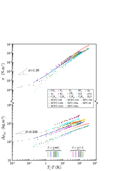
Figure 1: (Color online) a) Singular behavior (log-log scale) of the interfacial tension $\sigma$ (expressed in $\text{N}\,\text{m}^{-1}$) and b) singular behavior of the symmetrized order parameter density $\Delta\rho_{LV}$ (expressed in $\text{kg}\,\text{m}^{-3}$), as a function of the temperature distance $T_{c}-T$ (expressed in K), for one-component fluids (see text, Appendix A and references in Table I). Inserted Table gives colour indexation of each selected fluid. The temperature axis is labelled by vertical arrows which indicate the practical values $T=0.99\,T_{c}$ and $T=0.7\,T_{c}$, respectively (see text for details).

Now, we introduce the squared capillary length $\left(\ell_{Ca}\right)^{2}$ [also called the Sugden factor Sugden1921 ; Sugden1924 , noted $S_{g}$], related to $\sigma$ and $\Delta\rho_{LV}$ by

$$\left(\ell_{Ca}\right)^{2}\equiv S_{g}=\frac{2\sigma}{g\Delta\rho_{LV}},$$ (6)

where $g$ is the gravitational acceleration. Equation (6) expresses the balance between interfacial forces and volumic forces which define the shape and position of the liquid-gas interface in a gravity field of constant acceleration $g$. The asymptotic singular behavior of $S_{g}$ can be read as a Wegner-like expansion

$$S_{g}=S_{0}\left|\Delta\tau^{*}\right|^{\varphi}\left[1+\overset{i=\infty}{\underset{i=1}{\sum}}S_{i}\left|\Delta\tau^{*}\right|^{i\Delta}\right].$$ (7)

leading to the scaling law

$$\varphi=\phi-\beta$$ (8)

with $\varphi\approxeq 0.934$, and to the canonical amplitude combination

$$S_{0}=\frac{\sigma_{0}}{g\rho_{c}B}$$ (9)

Equations (4) to (9) are of basic interest as well for measurement techniques of interfacial properties as for theoretical crossover descriptions when the temperature distance to $T_{c}$ takes a finite value (see Appendix A).

The singular behavior of the Sugden factor $S_{g}$ as a function of the temperature distance $T_{c}-T$ was illustrated in Fig. 1 of Ref. Garrabos2007cal for about twenty pure compounds selected among inert gases, normal compounds and highly associating polar fluids. For the references of the $S_{g}$ and $\sigma$ data sources see the reviews of Refs. Gielen1984 ; LeNeindre2002 ; Garrabos2007cal ; Moldover1985 . Here, we have added the data sources Okada1986 ; Okada1987 ; Higashi1992 ; Okada1995 ; Moldover1988 ; Chae1990 of some hydrofluorocarbons (HFCs) and hydrocholorofluorocarbons (HCFCs) for related discussion in Appendix A. The raw data for the surface tension $\sigma\left(T_{c}-T\right)$ and the symmetrized order parameter density $\Delta\rho_{LV}\left(T_{c}-T\right)$ are reported in Figs. 1a and 1b, respectively. For the $\Delta\rho_{LV}$ data sources see for example the references given in Refs. Broseta2005 , LeNeindre2002 , and Okada1986 ; Okada1987 ; Higashi1992 ; Okada1995 ; Moldover1988 ; Chae1990 . In each case, the universal Ising-like slope of the asymptotic singular behavior appears compatible with the experimental results. From these figures, it is also expected about one-decade variation for each fluid-dependent amplitude $2\rho_{c}B\left(T_{c}\right)^{-\beta}$ and $\sigma_{0}\left(T_{c}\right)^{-\phi}$ of the leading terms of Eqs. (4) and (5), respectively.

As in the Sugden factor case Garrabos2007cal , it also appears evident that the raw data used in present Fig. 1 cover a large temperature range of the coexisting liquid-vapor phases since this range approaches the triple point temperature $T_{\text{TP}}$. We have then adopted the same practical distinction between asymptotic critical range and triple point region in the temperature axis, using vertical arrows for the temperature distances where $T=0.7\,T_{c}$ (i.e. the temperature distance where the fluid-dependent acentric factor $\omega$ is defined) and $T=0.99\,T_{c}$. In a large temperature range defined by $0.3\leq\left|\Delta\tau^{*}\right|\leq 1-\frac{T_{\text{TP}}}{T_{c}}$, the nonuniversal nature of each fluid is certainly dominant (see for example Appendix A), while, in the temperature range $\left|\Delta\tau^{*}\right|\leq 0.01$, the singular behavior descriptions by Wegner like expansions, and asymptotic two-scale-factor universality of their restricted two term form, hold.

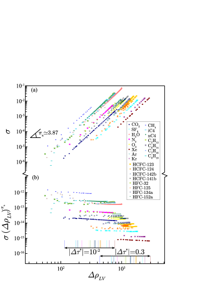
Figure 2: (Color on line) a) Asymptotic singular behavior of $\sigma$ as a function of $\Delta\rho_{LV}$ obtained from Fig. 1 b) As in a) for the confluent quantity $\frac{\sigma}{\left(\Delta\rho_{LV}\right)^{\pi_{a}}}$ (see caption of Fig. 1 and text for details and inserted Table for fluid colour indexation).

Selecting $\sigma$ and $\Delta\rho_{LV}$ measurements at identical values of $T_{c}-T$, we have constructed the corresponding $\sigma$-$\Delta\rho_{LV}$ data pairs. The singular behavior of $\sigma\left(\Delta\rho_{LV}\right)$ is illustrated in Fig. 2a, while the corresponding behavior of $\sigma\left(\Delta\rho_{LV}\right)^{-\pi_{a}}$ as a function of $\Delta\rho_{LV}$ is given in Fig. 2b, as usually made to enlighten the contribution of the confluent corrections to scaling and to have better estimation of the uncertainty attached to the value of the leading amplitude. Simultaneously, from xenon to n-octane, we also underline about a three-decade variation for the fluid-dependent amplitude of this quantity, leading to about a half-decade variation of the effective parachor (expressed in $\left[\text{J}\,\text{mole}^{-1}\,\text{m}^{3\pi_{a}-2}\right]$ unit when $\sigma$, $\Delta\rho_{LV}$, and $M_{\text{mol}}$ are expressed in $\left[\text{J}\,\text{m}^{-2}\right]$ (or $\left[\text{N}\,\text{m}^{-1}\right]$), $\left[\text{kg}\,\text{m}^{-3}\right]$, and $\left[\text{kg}\,\text{mole}^{-1}\right]$, respectively). Accordingly, by straightforward elimination of $\left|\Delta\tau^{*}\right|$ in Eqs. (4) to (7), we find the exact Ising-like asymptotic form

$$\begin{array}[]{cl}\sigma=&\left(\frac{P_{0}}{M_{\text{mol}}}\Delta\rho_{LV}\right)^{\pi_{a}}\\ &\left\{1+P_{1}\left(\Delta\rho_{LV}\right)^{\frac{\Delta}{\beta}}+\mathcal{O}\left[\left(\Delta\rho_{LV}\right)^{\frac{2\Delta}{\beta}}\right]\right\},\end{array}$$ (10)

where (as previously mentioned in the introduction part)

$$\pi_{a}=\frac{\phi}{\beta}=\frac{\varphi}{\beta}+1\approxeq 3.87,$$ (11)

The Ising-like asymptotic value $P_{0}$ of the effective parachor $P_{e}$ can be estimated using the leading terms of Eqs. (4) to (7) and reads

$$P_{0}=\left(\sigma_{0}\right)^{\frac{\beta}{\phi}}\frac{M_{\text{mol}}}{2\rho_{c}B}=\left(gS_{0}\right)^{\frac{\beta}{\phi}}\frac{M_{\text{mol}}}{2\left(\rho_{c}B\right)^{1-\frac{\beta}{\phi}}},$$ (12)

depending on the pair of selected variables, either $\left\{\sigma;\Delta\rho_{LV}\right\}$ or $\left\{S_{g};\Delta\rho_{LV}\right\}$. Equations (10) and (11) clearly demonstrate the critical scaling nature of Eq. (1), with an essential consequence: the parachor $P_{0}$ is a nonuniversal leading amplitude which must satisfy the two-scale-factor universality of the Ising-like universality class.

How to estimate the parachor appears thus as a basic question in a sense that only two nonuniversal leading amplitudes are sufficient to characterize the complete singular behavior of a one-component fluid when $T\rightarrow T_{c}$ and $\Delta\rho_{LV}\rightarrow 0$.

II.2 The basic set of fluid-dependent parameters

Fluid	$m_{\bar{p}}$	$T_{c}$	$p_{c}$	$\rho_{c}$	$\gamma_{c}^{{}^{\prime}}$	$\left(\beta_{c}\right)^{1}$	$\alpha_{c}$	$Z_{c}$	$Y_{c}$
	$\left(10^{-26}\,\text{kg}\right)$	$\left(\text{K}\right)$	$\left(\text{MPa}\right)$	$\left(\text{kg}\,\text{m}^{-3}\right)$	$\left(\text{MPa}\,\text{K}^{-1}\right)$	$\left(10^{-21}\,\text{J}\right)$	$\left(\text{nm}\right)$
Ar	$6.6335$	$150.725$	$4.865$	$535$	$0.19025$	$2.08099$	$0.7535$	$0.289871$	$4.89423$
Kr	$13.9153$	$209.286$	$5.500$	$910$	$0.1562$	$2.8895$	$0.8069$	$0.291065$	$4.94372$
Xe	$21.8050$	$289.740$	$5.840$	$1113$	$0.1185$	$4.0003$	$0.8815$	$0.286010$	$4.87914$
N2	$4.6517$	$126.200$	$3.400$	$314$	$0.1645$	$1.74258$	$0.8002$	$0.289078$	$5.10585$
O2	$5.3136$	$154.58$	$5.043$	$436$	$0.1953$	$2.13421$	$0.7508$	$0.287972$	$4.98641$
CO2	$7.3080$	$304.107$	$7.732$	$467.8$	$0.173$	$4.19907$	$0.8289$	$0.274352$	$6.13653$
SF6	$24.2555$	$318.687$	$3.76$	$741.5$	$0.084$	$4.40062$	$1.054$	$0.281243$	$6.11960$
H2O	$2.9969$	$647.067$	$22.046$	$322.8$	$0.2676319$	$8.93373$	$0.7400$	$0.229117$	$6.85520$
C2H4	$4.658$	$282.345$	$5.042$	$214.5$	$0.11337$	$3.89820$	$0.91781$	$0.28131$	$5.34856$
CH4	$2.6640$	$190.564$	$4.59920$	$162.7$	$0.14746$	$2.63102$	$0.8301$	$0.285752$	$4.981927$
C2H6	$4.99324$	$305.322$	$4.872$	$206.58$	$0.10304$	$4.21554$	$0.95290$	$0.27935$	$5.45505$
C3H8	$7.32248$	$369.825$	$4.2462$	$220$	$0.077006$	$5.106$	$1.063$	$0.27679$	$5.70688$
n-C4H10	$9.6518$	$425.38$	$3.809$	$229$	$0.0643$	$5.87301$	$1.155$	$0.273352$	$6.17774$
i-C4H10	$9.6518$	$407.85$	$3.65$	$225$	$0.0643$	$5.63102$	$1.155$	$0.278056$	$6.18173$
C5H12	$11.9808$	$469.70$	$3.3665$	$232$	$0.0511$	$6.48491$	$1.244$	$0.270875$	$6.12956$
C6H14	$14.3100$	$507.85$	$3.0181$	$234$	$0.043658$	$7.00666$	$1.319$	$0.266670$	$6.30719$
C7H16	$16.6393$	$540.13$	$2.727$	$234$	$0.038068$	$7.45731$	$1.398$	$0.262180$	$6.64356$
C8H18	$18.9685$	$568.88$	$2.486$	$232$	$0.033768$	$7.85424$	$1.467$	$0.258978$	$6.82776$
HFC-32	$8.6386$	$351.26$	$5.782$	$423$	$0.124088$	$4.849676$	$0.9431$	$0.243384$	$6.53842$
HCFC-123	$25.3948$	$456.82$	$3.666$	$554$	$0.005711$	$6.30764$	$1.1982$	$0.266439$	$6.11647$
HCFC-124	$22.6622$	$395.35$	$3.615$	$566$	$0.063205$	$5.45840$	$1.1473$	$0.265179$	$5.91234$
HFC-125	$19.9301$	$339.17$	$3.618$	$568$	$0.078665$	$4.68275$	$1.0898$	$0.271100$	$6.37446$
HFC-134a	$16.9426$	$374.30$	$4.065$	$512.7$	$0.083109$	$5.16777$	$1.0833$	$0.259940$	$6.65260$
HCFC-141b	$19.42$	$477.31$	$4.250$	$460$	$0.060522$	$6.58998$	$1.1575$	$0.272268$	$5.79119$
HCFC-142b	$16.6876$	$410.26$	$4.041$	$447$	$0.071972$	$5.66426$	$1.1191$	$0.266338$	$6.30691$
HFC-152a	$10.9680$	$386.41$	$4.512$	$369$	$0.086345$	$5.33497$	$1.0574$	$0.251384$	$6.39463$

Table 1: Critical parameters for the selected one-components fluids.

As proposed by Garrabos Garrabos1982 ; Garrabos1985 , a phenomenological response to the above basic question relies on the hypothesis that the set

$$Q_{c,a_{\bar{p}}}^{\text{min}}=\left\{p_{c},v_{\bar{p},c},T_{c},\gamma_{c}^{{}^{\prime}}\right\},$$ (13)

of four critical coordinates which localize the gas-liquid critical point on the $p,v_{\bar{p}},T$ phase surface, contains all the needed critical information to calculate any nonuniversal leading amplitude of the selected fluid (here neglecting the quantum effects Garrabos2006qe to simplify the presentation). The mass $m_{\bar{p}}$ of each molecule is also hypothesized known to infer the total amount $N$ of fluid particles by measurements of the fluid total mass $M=N_{A}m_{\bar{p}}$. $p$ ($p_{c}$) is the (critical) pressure. $v_{\bar{p}}=\frac{\bar{v}}{N_{A}}=\frac{m_{\bar{p}}}{\rho}$ ($v_{\bar{p},c}=\frac{m_{\bar{p}}}{\rho_{c}}$) is the molecular volume (critical volume). The total volume $V=Nv_{\bar{p}}$ is the extensive variable conjugated to $p$. $\gamma_{c}^{{}^{\prime}}=\left[\left(\frac{\partial p}{\partial T}\right)_{v_{\bar{p},c}}\right]_{\text{CP}}$ is the common critical direction in the $p;T$ diagram of the critical isochore and the saturation pressure curve $p_{\text{sat}}\left(T\right)$ at critical point (CP), thus defined by

$$\gamma_{c}^{{}^{\prime}}=\left(\frac{\partial p}{\partial T}\right)_{\rho_{c},T\rightarrow T_{c}^{+}}=\left(\frac{dp_{\text{sat}}}{dT}\right)_{T\rightarrow T_{c}^{-}}$$ (14)

Rewriting Eq. (13) as a four-scale-factor set

$$Q_{c}^{\text{min}}=\left\{\beta_{c}^{-1},\alpha_{c},Z_{c},Y_{c}\right\}$$ (15)

where,

$$\beta_{c}^{-1}=k_{B}T_{c}\sim\left[\text{energy}\right]$$ (16)

$$\alpha_{c}=\left(\frac{k_{B}T_{c}}{p_{c}}\right)^{\frac{1}{d}}\sim\left[\text{length}\right]$$ (17)

$$Z_{c}=\frac{p_{c}m_{\bar{p}}}{k_{B}T_{c}\rho_{c}}$$ (18)

$$Y_{c}=\gamma_{c}^{{}^{\prime}}\frac{T_{c}}{p_{c}}-1$$ (19)

we introduce the energy unit [$\beta_{c}^{-1}$], the length unit [$\alpha_{c}$], the (isothermal) scale factor [$Z_{c}$] of the order parameter density [see Eq. (3)] along the critical isothermal line, and the (isochoric) scale factor [$Y_{c}$] of the temperature field [see Eq. (2)] along the critical isochoric line.

Table 1 provides values of the critical parameters involved in Eqs. (13) and (15) for the $23$ pure fluids selected in this paper.

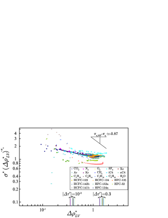
Figure 3: (Color online) Singular behavior (log-log scale) of the dimensionless quantity $\frac{\sigma^{*}}{\left(\Delta\tilde{\rho}_{LV}\right)^{\pi_{a}}}$ as a function of the symmetrized order parameter density $\Delta\tilde{\rho}_{LV}$; inserted slope: direction difference $\pi_{a,\text{MF}}-\pi_{a}=-0.87$ from $\pi_{a,\text{MF}}=3$ (see text); arrow sets in lower horizontal axis: $\left|\Delta\tau^{*}\right|=10^{-2}$ and $\left|\Delta\tau^{*}\right|=0.3$ (see text and caption of 1); Inserted Table gives the fluid colour indexation.

Indeed, our dimensional scale units of energy $\left(\beta_{c}\right)^{-1}$ [Eq. (16)], and length $\alpha_{c}$ [Eq. (17)], provide equivalent description as $T_{c}$ and $p_{c}$ of the basic (2-parameter) corresponding-states principle. The customary dimensionless forms of $\sigma$ and $\Delta\rho_{LV}$ are $\sigma^{*}=\left(\alpha_{c}\right)^{d-1}\beta_{c}\sigma$ and $\Delta\tilde{\rho}_{LV}=\frac{\Delta\rho_{LV}}{2\rho_{c}}$. As for the Sugden factor case, Fig. 3 gives distinct curves of $\sigma^{*}\left(\Delta\tilde{\rho}_{LV}\right)^{-\pi_{a}}$ as a function of $\Delta\tilde{\rho}_{LV}$, which confirms the failure of any description based on the two-parameter corresponding-states principle. Moreover, the direction difference $\pi_{a,\text{MF}}-\pi_{a}\approxeq-0.87$ with a classical power law of mean field exponent $\pi_{a,\text{MF}}=3$ also disagrees with experimental trends at large temperature distance, as illustrated in Fig. 3.

On the other hand, the set $Q_{c}^{min}$ [Eqs. (15) to (19)] conforms to the general description provided from appropriate 4-parameter corresponding-states modelling, as mentioned in our introductive part. For example, we retrieve that the scale factor $Y_{c}$ [Eq. (19)] is related to the Riedel factor $\alpha_{c,R}=\gamma_{c}^{{}^{\prime}}\frac{T_{c}}{p_{c}}$ by $Y_{c}+1=\alpha_{c,R}$, as mentioned in our introductive part. However, as we will extensively show in this paper, the scale dilatation approach brings a theoretical justification to these critical parameters, initially introduced only to build extended corresponding-states principle.

First, the microscopic meaning of $\left(\beta_{c}\right)^{-1}$ and $\alpha_{c}$, related to the minimum value [$\epsilon$$\sim$$\left(\beta_{c}\right)^{-1}$], of the interaction energy between particle pairs at equilibrium position [$r_{e}$$\sim$$\frac{1}{2}$$\alpha_{c}$] , takes primary importance. Thus, $\alpha_{c}$ appears as the mean value of the finite range of the attractive interaction forces between particles. So that,

$$v_{c,I}=\left(\alpha_{c}\right)^{d}$$ (20)

is the microscopic volume of the critical interaction cell at the exact ($T=T_{c}$ and $p=p_{c}$) critical point. Using thermodynamic properties per particle, it is straight to show that the critical interaction cell is filled by the critical number of particles

$$N_{c,I}=\frac{1}{Z_{c}}$$ (21)

since, rewriting Eq. (18), we have

$$\frac{k_{B}T_{c}}{p_{c}}=v_{c,I}=N_{c,I}\times v_{\bar{p},c}=\frac{1}{Z_{c}}\times\frac{m_{\bar{p}}}{\rho_{c}}$$ (22)

Second, since in the critical phenomena description only one length scale unit is needed to express correctly the non-trivial length dimensions of thermodynamic and correlation variables Privman1991 , the above microscopic analysis is of primary importance. By chosing $\alpha_{c}$, the two dimensionless scale factors $Z_{c}$ and $Y_{c}$ are then characteristic properties of the critical interaction cell of each one-component fluid. Specially, $\frac{1}{Z_{c}}$ takes similar microscopic nature of the coordination number in the lattice description of the three-dimensional Ising systems, while $\alpha_{c}$ takes similar microscopic nature of their lattice spacing $a_{\text{Ising}}$.

On the basis of this microscopic understanding, we are now in position to estimate the Ising-like parachor from $Q_{c}^{\text{min}}$, using scale dilatation of the physical fields Garrabos1982 .

Fluid	$\phi_{e}$	$\sigma_{0,e}$	Ref.	$\sigma_{0}$	$\mathcal{Z}_{\sigma,\text{exp}}$	$\delta\mathcal{Z}_{\sigma,\text{exp}}$	Ref
		$\left(10^{-3}\,\text{N}\,\text{m}^{-1}\right)$		$\left(10^{-3}\,\text{N}\,\text{m}^{-1}\right)$		$\%$
Ar				$31.55$	$1.162$	$0.5$	Moldover1988
				$30.48$	$1.123$	$-2.9$	Gielen1984
	$1.281$	$38.07$	Stansfield1958	$31.42$	$1.158$	$0.1$	This work
	$1.277$	$37.78$	Sprow1966	$31.76$	$1.170$	$1.2$	This work
Xe				$45.69$	$1.179$	$2.0$	Moldover1985
				$45.61$	$1.177$	$1.8$	Gielen1984
	$1.302\left(\pm 0.006\right)$	$62.9\left(\pm 1.8\right)$	Zollweg1971	$47.1$	$1.215$	$5.1$	This work
	$1.290$	$53.9$	Smith1967 (from Leadbetter1965 )	$42.68$	$1.101$	$-4.8$	This work
	$1.287\left(\pm 0.017\right)$	$54.6\left(\pm 0.1\right)$	Smith1967	$43.83$	$1.131$	$-2.2$	This work
N2				$25.75$	$1.212$	$4.8$	Gielen1984
O2				$34.04$	$1.186$	$2.6$	Gielen1984
CO2				$70.05$	$1.209$	$4.6$	Moldover1985
				$65.93$	$1.138$	$-1.5$	Gielen1984
	$1.26$	$76$	Gielen1984 (from Herpin1973 )	$69.1$	$1.193$	$3.2$	This work
	$1.281$	$84.72$	Grigull1969	$69.92$	$1.207$	$4.4$
SF6				$47.85$	$1.230$	$6.4$	Moldover1985
				$44.09$	$1.134$	$-1.9$	Gielen1984
	$1.285\left(\pm 0;016\right)$	$55.13\left(\pm 2.6\right)$	Wu1973	$46$	$1.183$	$2.3$	Gielen1984
	$1.285\left(\pm 0;016\right)$	$55.13\left(\pm 2.6\right)$	Wu1973	$44.64$	$1.148$	$-0.7$	This work
	$1.286$	$54.28$	Rathjen1980	$43.78$	$1.126$	$-2.6$	This work
CBrF3	$1.279$	$54.05$	Rathjen1980	$45.02$	$1.106$	$-4.3$
CClF3	$1.30$	$58.84$	Grigull1969	$44.5$	$1.135$	$-1.8$	This work
	$1.283$	$52.53$	Rathjen1980	$42.96$	$1.096$	$-5.2$	This work
CHClF2	$1.283$	$69.03$	Rathjen1980	$56.44$	$1.139$	$-1.5$	This work
CCl2F2	$1.283$	$59.63$	Rathjen1980	$48.76$	$1.172$	$1.4$	This work
CCl3F	$1.263$	$63.24$	Rathjen1980	$56.78$	$1.196$	$3.5$	This work
H2O				$218$	$1.135$	$-1.8$	Moldover1985
				$220.7$	$1.149$	$-0.6$	Gielen1984
CH4				$30.22$	$1.012$	$-12.4$	Gielen1984
C2H4				$45.08$	$1.166$	$0.8$	Moldover1985
C2H6				$45.15$	$1.145$	$-1.0$	Moldover1985
i-C4H10				$45.9$	$1.159$	$0.2$	Moldover1988
$mean$					$1.167$	$1.0$
$standard$					$0.062$	$5.4$

Table 2: Effective values of the critical exponent (column 2) and asymptotic amplitudes of interfacial tension (column 3) from references given in column 4. Related estimations of the leading asymptotic amplitude $\sigma_{0}$ (column 5) (see text for details). Calculated values of the corresponding master amplitudes $\mathcal{Z}_{\sigma,\text{exp}}=\mathcal{\sigma}_{0}\left(\alpha_{c}\right)^{2}\beta_{c}\left(Y_{c}\right)^{-\phi}$ (column 6) of the master interfacial tension (see Table 1 for the values of $\alpha_{c}$, $\beta_{c}$, and $Y_{c}$). The % differences $\delta\mathcal{Z}_{\sigma,\text{exp}}=100\left(\frac{\mathcal{Z}_{\sigma,\text{exp}}}{\mathcal{Z}_{\sigma}}-1\right)$ from the values $\mathcal{Z}_{\sigma}=1.156$ estimated from universal amplitude combinations are given in column 7. For references see column 8.

II.3 The scale dilatation of the physical variables

The asymptotic master critical behavior for interfacial properties when $T\rightarrow T_{c}$ and $\Delta\rho_{LV}\rightarrow 0$, can be observed by using the following dimensionless physical quantities

$$\Delta\tau^{*}=k_{B}\beta_{c}\left(T_{c}-T\right)$$ (23)

$$\Delta\mu_{\bar{p}}^{*}=\beta_{c}\left(\mu_{\bar{p}}-\mu_{\bar{p},c}\right)$$ (24)

$$\Delta m^{*}=\left(\alpha_{c}\right)^{d}\left(n-n_{c}\right)=\left(Z_{c}\right)^{-1}\Delta\tilde{\rho}$$ (25)

and the following master (rescaled) quantities,

$$\mathcal{T}^{*}=Y_{c}\left|\Delta\tau^{*}\right|$$ (26)

$$\mathcal{H}^{*}=\left(Z_{c}\right)^{-\frac{d}{2}}\Delta\mu_{\bar{p}}^{*}=\left(Z_{c}\right)^{-\frac{1}{2}}\Delta\tilde{\mu}_{\rho}$$ (27)

$$\mathcal{M}^{*}=\left(Z_{c}\right)^{\frac{d}{2}}\Delta m^{*}=\left(Z_{c}\right)^{\frac{1}{2}}\Delta\tilde{\rho}$$ (28)

$$\Sigma^{*}\equiv\sigma^{*}$$ (29)

$$\mathcal{S}_{g^{*}}^{*}=g^{*}\left(Z_{c}\right)^{-\frac{3}{2}}\left(\ell_{Ca}^{*}\right)^{d-1}$$ (30)

where, in Eqs. (26) to (30), we have only used the two scale factors $Y_{c}$ and $Z_{c}$ to rescale the dimensionless quantities, with $\sigma^{*}=\left(\alpha_{c}\right)^{d-1}\beta_{c}\sigma$; $\ell_{Ca}^{*}=\left(\alpha_{c}\right)^{-1}\ell_{Ca}$ and $g^{*}=m_{\bar{p}}\beta_{c}\alpha_{c}g$. $\mu_{\bar{p}}$ ($\mu_{\bar{p},c}$) is the molecular chemical potential (critical molecular chemical potential). $n$ ($n_{c}$) is the number density (critical number density). The normalized variable $n=\frac{N}{V}$, where $\mu_{\bar{p}}$ is conjugated to the total amount of matter $N$, is then related to the order parameter (number) density expressing thermodynamic properties per molecule. As mentionned in the introduction, the (mass) density $\rho=\frac{M}{V}$, where $\mu_{\rho}$ is conjugated to the total mass of matter $M$, is related to the order parameter density, but expressing thermodynamic properties per volume unit. Here we have noted $\mu_{\rho}=\frac{\mu_{\bar{p}}}{m_{\bar{p}}}$ the chemical potential per mass unit. The dimensionless form of $\mu_{\rho}$ is $\tilde{\mu}_{\rho}=\mu_{\rho}\frac{\rho_{c}}{p_{c}}$, while the one of $\mu_{\bar{p}}$ is $\mu_{\bar{p}}^{*}=\mu_{\bar{p}}\beta_{c}$, with $\frac{1}{Z_{c}}\mu_{\bar{p}}^{*}=\tilde{\mu}_{\rho}$. $g$ is the gravitational acceleration needed to perform conventional measurements by capillary rise or drop techniques Sugden1924 ; Rowlinson 1984 . $g^{*}$ is the dimensionless gravitational acceleration, where we have used $\alpha_{c}\left(m_{\bar{p}}\beta_{c}\right)^{\frac{1}{2}}\sim\left[\frac{\text{mass}\left(\text{length}\right)^{2}}{\text{energy}}\right]^{\frac{1}{2}}$ as a time unit.

In Eqs. (26) and (27), $Y_{c}$ and $Z_{c}$ are two independent scale factors that dilate the temperature field along the critical isochore and the ordering field along the critical isotherm, respectively. These Eqs. (26) and (27) are formally analogous to analytical relations Wilson1971 linking two relevant fields of the so-called $\Phi_{d=3}^{4}\left(n=1\right)$ model with two physical variables of a real system belonging to the universality class. That implicitely imposes that only a single microscopic length is characteristic of the system Privman1991 , which then can be related to the inverse coupling constant of the model taking appropriate length dimension, precisely for the $d=3$ case. When a single length is the common unit to the thermodynamic and correlation functions, the singular part of free energy of any system belonging to the universality class remains proportional to a universal quantity which generally refers to the (physical) value of the critical temperature. In the case of one-component fluids, the single characteristic length originates from thermodynamic considerations [see above $\alpha_{c}$ of Eq. (17)]. Accordingly, the universal singular free energy density is expressed in units of $\left(\beta_{c}\right)^{-1}=k_{B}T_{c}$ [see Eq. (16)]. The master fields $\mathcal{T}^{*}$ and $\mathcal{H}^{*}$ have similar Ising-like nature to the renormalized fields $t$ and $h$ in field theory applied to critical phenomena.

II.4 Master crossover behavior for interfacial properties of the one-component fluid subclass

The observation of the critical crossover behavior of a master property $\mathcal{P}^{*}$ in a $\mathcal{P}^{*}-\mathcal{T}^{*}$ diagram, generates a single curve which can be described by a master Wegner-like expansion $\mathcal{P}^{*}\left(\mathcal{T}^{*}\right)$. Asymptotically, i.e. for $\mathcal{T}^{*}\rightarrow 0$, the universal features of fluid singular behaviors are at least valid in the Ising-like preasymptotic domain Bagnuls1985 ; Garrabos2006gb where only two asymptotic amplitudes and one first confluent amplitude characterize each one-component fluid. In our present formulation of the liquid-vapor interfacial properties, we define $\mathcal{M}_{LV}^{*}=\left(Z_{c}\right)^{\frac{3}{2}}\Delta m_{LV}^{*}=\left(Z_{c}\right)^{\frac{1}{2}}\Delta\tilde{\rho}_{LV}$, $\Delta m_{LV}^{*}=\left(\alpha_{c}\right)^{d}\left(n_{L}-n_{V}\right)=\left(Z_{c}\right)^{-1}\Delta\tilde{\rho}_{LV}$, $\Delta\tilde{\rho}_{LV}=\frac{\rho_{L}-\rho_{V}}{2\rho_{c}}$, and we introduce the following master equations of interest, here restricted to the first order of the critical confluent correction to scaling to be in conformity with the above universal faetures,

$$\mathcal{M}_{LV}^{*}=\mathcal{Z}_{M}\left(\mathcal{T}^{*}\right)^{\beta}\left[1+\mathcal{Z}_{M}^{\left(1\right)}\left(\mathcal{T}^{*}\right)^{\Delta}+...\right]$$ (31)

$$\Sigma^{*}=\mathcal{Z}_{\sigma}\left(\mathcal{T}^{*}\right)^{\phi}\left[1+\mathcal{Z}_{\sigma}^{\left(1\right)}\left(\mathcal{T}^{*}\right)^{\Delta}+...\right]$$ (32)

$$\mathcal{S}_{g^{*}}^{*}=\mathcal{Z}_{S}\left(\mathcal{T}^{*}\right)^{\varphi}\left[1+\mathcal{Z}_{S}^{\left(1\right)}\left(\mathcal{T}^{*}\right)^{\Delta}+...\right]$$ (33)

with their interrelation [see Eqs. (8) and (6)]

$$\mathcal{S}_{g^{*}}^{*}=\frac{\Sigma^{*}}{\mathcal{M}_{LV}^{*}}$$ (34)

The master asymptotic behaviors of $\mathcal{M}_{LV}^{*}$ and $\mathcal{S}_{g^{*}}^{*}$ as a function of $\mathcal{T}^{*}$ were observed and analyzed in Refs. Garrabos2002 and Garrabos2007cal for several pure fluids. The corresponding master amplitudes take the values $\mathcal{Z}_{M}\approxeq 0.468\,\left(\pm 0.001\right)$ and $\mathcal{Z}_{S}\approxeq 2.47\,\left(\pm 0.17\right)$ (for the quoted error-bars see Refs. Garrabos2002 ; Garrabos2007cal ). ¿From Eq. (34), the leading master amplitude for the surface tension case is then $\mathcal{\mathcal{Z}_{\sigma}}=\mathcal{Z}_{M}\mathcal{Z}_{S}\approxeq 1.156\,\left(\pm 0.087\right)$. Here, using a method similar to the one applied to the Sugden factor case, we show in Table 2 that this master value is compatible with the results obtained from experiments performed sufficiently close to the critical point. Therefore, only surface tension measurements already analyzed by Moldover Moldover1985 and Gielen et al Gielen1984 are considered. The respective effective values $\phi_{e}$ and $\mathcal{\sigma}_{0,e}$ of the exponent-amplitude pair corresponding to data fits by an effective power law $\sigma=\sigma_{0,e}\left|\Delta\tau^{*}\right|^{\phi_{e}}$ are reported in columns 2 and 3, when needed for the present analysis (see the corresponding Refs. Stansfield1958 ; Leadbetter1965 ; Sprow1966 ; Smith1967 ; Zollweg1971 ; Herpin1973 ; Wu1973 ; Grigull1969 ; Rathjen1980 in column 4). The estimated values of the leading amplitude $\sigma_{0}$ for the Ising value $\phi\approxeq 1.260$ of the critical exponent are given in column 5. The references reported in column 8 precise the origin of these estimations, which are mainly dependent on the accuracy of the interfacial property measurements in the vicinity of $\left|\Delta\tau^{*}\right|\simeq 0.01$. For example, in the present work we have estimated $\sigma_{0}$ by the following relation $\sigma_{0}=\frac{\mathcal{\sigma}_{0,e}\left(0.01\right)^{\phi_{e}-1.260}}{1.1}$, using data sources of columns 2 and 3. Our estimation is then compatible with surface tension measurements at $\left|\Delta\tau^{*}\right|=0.01$, neglecting confluent corrections in Sugden factor measurements Garrabos2007cal , and averaging (for all the selected fluids) the confluent correction contributions in density measurements to $10\%$ at this finite distance to the critical temperature Garrabos2002 . The values of $\mathcal{Z}_{\sigma,\text{exp}}=\mathcal{\sigma}_{0}\left(\alpha_{c}\right)^{2}\beta_{c}\left(Y_{c}\right)^{-\phi}$ (column 6) calculated from these $\mathcal{\sigma}_{0}$ estimations are in close agreement with our master value $\mathcal{Z}_{\sigma}=1.156$. The residuals $\delta\mathcal{Z}_{\sigma,\text{exp}}=100\left(\frac{\mathcal{Z}_{\sigma,\text{exp}}}{\mathcal{Z}_{\sigma}}-1\right)$ (column 7) expressed in %, are of the same order of magnitude than the experimental uncertainties [see for example Refs. Moldover1985 and Gielen1984 ]. We note that the $+1\%$ residuals between the experimental mean value $\left\langle\mathcal{Z}_{\sigma,\text{exp}}\right\rangle=1.167$ and the estimated master one $\mathcal{Z}_{\sigma}=1.156$, have a standard deviation ($\pm 5.4\%$) comparable to the experimental uncertainties ($\sim 7.5\%$). However, this good agreement on the central value is noticeable in regards to significant contributions of confluent corrections, as reflected by the effective exponent values $\phi_{e}\approx 1.28-1.31$ larger than $\phi\approxeq 1.260$ at finite distance from $T_{c}$ (see also a complementary discussion related to the analysis of data at large distance from $T_{c}$ given in Appendix A).

Similarly, each confluent amplitude $\mathcal{Z}_{M}^{\left(1\right)}$, $\mathcal{Z}_{\sigma}^{\left(1\right)}$, and $\mathcal{Z}_{S}^{\left(1\right)}$, takes a master constant value for all one-component fluids. Among all $\mathcal{Z}_{P}^{\left(1\right)}$, only one is independent and characteristic of the pure fluid subclass.

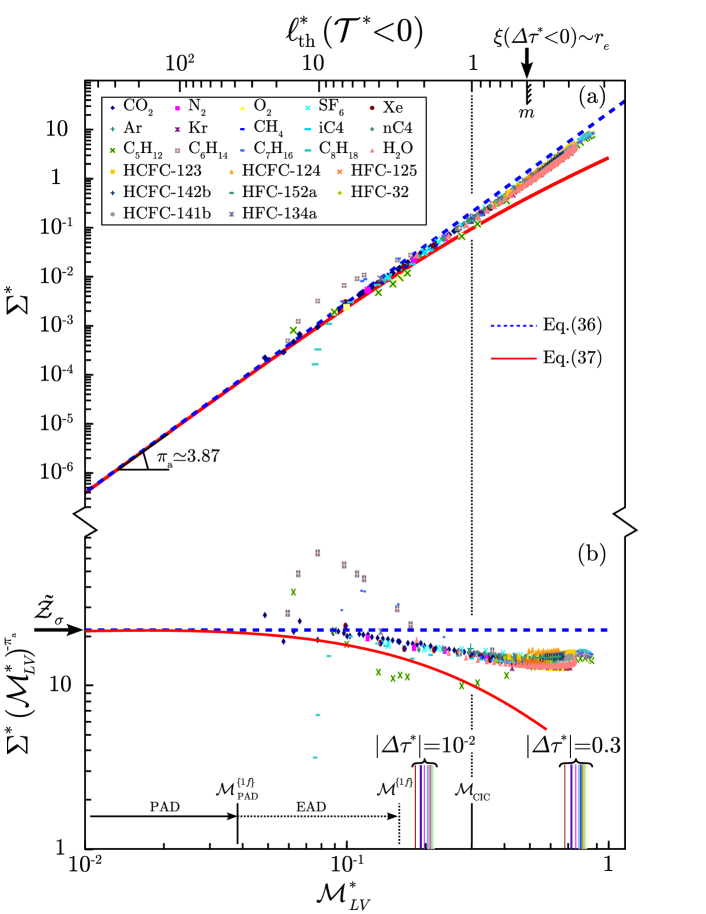
Figure 4: (Colour online) a) Master singular behavior (log-log scale) of the renormalized surface tension $\Sigma^{*}=\sigma^{*}$ [Eq. (29)], as a function of the renormalized (symmetrized) order parameter density $\mathcal{M}_{LV}^{*}$ in the nonhomogeneous domain [see Eq. (28) and text]; b) As in a) for the “confluent” quantity $\frac{\Sigma^{*}}{\left(\mathcal{M}_{LV}^{*}\right)^{\pi_{a}}}$ (see text). In a) and b): Dashed blue curve: Eq. (36); full red curve: (37); full arrow with label PAD:$\mathcal{M}_{LV}^{*}<\mathcal{M}_{\text{PAD}}^{\left\{1f\right\}}$ extension of the preasymptotic domain; dotted arrow with label EAD: $\mathcal{M}_{LV}^{*}<\mathcal{M}^{\left\{1f\right\}}$extension of the extended asymptotic domain; The graduation of the upper horizontal axis gives $\ell^{*}\left(\mathcal{T}^{*}<0\right)$ calculated from theoretical crossover (see text and Ref. Garrabos2007cal ); arrow sets in lower horizontal axis:$\left|\Delta\tau^{*}\right|=10^{-2}$ and $\left|\Delta\tau^{*}\right|=0.3$, respectively; Inserted Table gives the fluid color indexation.

Despite their great interest for the validation of theoretical predictions, the exact forms of Eqs. (31) to (33) are not essential to understand the independent scaling role of the two scale factors $Y_{c}$ and $Z_{c}$. Moreover, our present interest is mainly focused on the scaling nature of $Z_{c}$. More precisely, by a variable exchange from $\Delta\tilde{\rho}$ to $\left(Z_{c}\right)^{\frac{1}{2}}\Delta\tilde{\rho}$, the expected master behavior must be observed when the master order parameter density $\mathcal{M}^{*}=\left(Z_{c}\right)^{\frac{1}{2}}\Delta\tilde{\rho}$ is used as a $x$- axis, generating then each “collapsed” curve of master equation $\mathcal{P}^{*}\left(\mathcal{M}^{*}\right)$ in the Ising-like preasymptotic domain, i.e. for $\mathcal{M}^{*}\rightarrow 0$. Usually, such a master behavior of the singular fluid (bulk) properties occurs along the critical isothermal line $T=T_{c}$, i.e., for $\mathcal{T}^{*}=\Delta\tau^{*}=0$, which provides disappearing of the scale factor $Y_{c}$ and which only preserves the contribution of the scale factor $Z_{c}$ in the determination of the fluid-dependent amplitudes Garrabos1985 ; Garrabos1986 . However, in the nonhomogeneous domain, the order parameter density spontaneously takes a finite value to distinguish the two coexisting phases in equilibrium. Thus, along the critical isochore, it is also possible to observe the master behavior of any singular (interfacial) property expressed as a function of the “symmetrized” order parameter density, starting with the surface tension as a typical example.

¿From $\sigma$ and $\Delta\rho_{LV}$ at identical $T_{c}-T$, we can construct data points of master coordinates $\Sigma^{*}=\left(\alpha_{c}\right)^{d-1}\beta_{c}\sigma$ and $\mathcal{M}_{LV}^{*}=\left(Z_{c}\right)^{\frac{1}{2}}\frac{\Delta\rho_{LV}}{2\rho_{c}}$ in the $\Sigma^{*}$-$\mathcal{M}_{LV}^{*}$ diagram. As illustrated in Fig. 4a, all these data collapse to define a master behavior of $\Sigma^{*}\left(\mathcal{M}_{LV}^{*}\right)$ for $\mathcal{M}_{LV}^{*}\rightarrow 0$. This collapse is well-enlightened in Fig. 4b which illustrates the corresponding master behavior of $\Sigma^{*}\left(\mathcal{M}_{LV}^{*}\right)^{-\pi_{a}}$, without any reference to a fitting master equation. To have a better appreciation of the real temperature range of the VLE domain, the values of $\left|\Delta\tau^{*}\right|=0.01$ and $\left|\Delta\tau^{*}\right|=0.3$ are also given by (fluid-dependent) arrows in the $\mathcal{M}_{LV}^{*}$ axis.

Obviously, using Wegner-like expansions to eliminate $\mathcal{T}^{*}$ between Eqs. (31) and (32), the leading power law of $\Sigma^{*}$ as a function of $\mathcal{M}_{LV}^{*}$ reads as follows

$$\Sigma^{*}=\mathcal{\widetilde{Z}}_{\sigma}\left(\mathcal{M}_{LV}^{*}\right)^{\frac{\phi}{\beta}}\left\{1+\mathcal{O}\left[\left(\mathcal{M}_{LV}^{*}\right)^{\frac{\Delta}{\beta}}\right]\right\}$$ (35)

where $\mathcal{\widetilde{Z}}_{\sigma}=\frac{\mathcal{Z}_{\sigma}}{\left(\mathcal{Z}_{M}\right)^{\frac{\phi}{\beta}}}\approxeq 21.88$. This asymptotical amplitude is illustrated by an arrow in the vertical axis of Fig. 4b and the related horizontal dashed (blue) line indicates clearly that the observed master behavior at finite distance to the critical point seems in “asymptotical” agreement.

In addition, the formal analogy between the basic hypotheses of the renormalization theory and the scale dilatation method makes also easy to probe that the effective fluid crossover behavior estimated from the massive renormalization scheme is consistent with the asymptotical power law of Eq. (35)] when $\mathcal{M}_{LV}^{*}\rightarrow 0$. As a matter of fact, along the critical isochore, the theoretical estimations of the fluid master behaviors in a whole thermal field range $0<\left|\mathcal{T}^{*}\right|<\infty$ can be made using the recent modifications Garrabos2006gb ; Garrabos2006mcf of the crossover functions calculated by Bagnuls and Bervillier Bagnuls2002 for the classical-to-critical crossover of the Ising-like universality class. However, as already noted in the Sugden factor case Garrabos2007cal , the theoretical function giving the classical-to-critical crossover of the interfacial tension is not available. Thus, to estimate $\Sigma_{\text{th}}^{*}$, we must use two alternative routes, introducing the theoretical estimations of either $\mathcal{M}_{\text{th}}^{*}\left(\mathcal{T}^{*}<0\right)$ or $\ell_{\text{th}}^{*}\left(\mathcal{T}^{*}<0\right)$.

A first straightforward route consists in using as an entry quantity the theoretical value $\mathcal{M}_{\text{th}}^{*}$ of the master order parameter density, admitting then that $\mathcal{M}_{\text{th}}^{*}\left(\mathcal{T}<0\right)\equiv\mathcal{M}_{LV}^{*}\left(\left|\mathcal{T}\right|\right)$, an identity already validated at least in the preasymptotic domain $\left|\mathcal{T}\right|\lesssim\mathcal{L}_{\text{PAD}}^{\left\{1f\right\}}$ (see Ref. Garrabos2002 ). As a result, the theoretical parachor function reads as follows

$$\Sigma_{\text{th,}\mathcal{M}}^{*}=\mathcal{\widetilde{Z}}_{\sigma}\left(\mathcal{M}_{\text{th}}^{*}\right)^{\frac{\phi}{\beta}}$$ (36)

justifying precisely the dashed blue curves in Figs. 4a and b, for the complete $\mathcal{M}_{LV}^{*}$-range. Unfortunately, at large values of $\mathcal{T}^{*}$, the theoretical function $\mathcal{M}_{\text{th}}^{*}\left(\mathcal{T}^{*}<0\right)$ is certainly not able to reproduce the experimental behavior of $\mathcal{M}_{LV}^{*}\left(\left|\mathcal{T}\right|\right)$ and, in the absence of this dedicated analysis, we cannot indicate easily the true extension of the $\mathcal{M}_{LV}^{*}$-range where the identity $\mathcal{M}_{\text{th}}^{*}\left(\mathcal{T}<0\right)\equiv\mathcal{M}_{LV}^{*}\left(\left|\mathcal{T}\right|\right)$ holds.

To pass round this difficulty, a second route combines the theoretical functions $\ell_{\text{th}}^{*}\left(\mathcal{T}^{*}<0\right)$ and $\mathcal{M}_{\text{th}}^{*}\left(\mathcal{T}^{*}<0\right)$ in a whole thermal field range $0<\left|\mathcal{T}^{*}\right|<\infty$, to infer numerically the function $\ell_{\text{th}}^{*}\left(\mathcal{M}_{\text{th}}^{*}\right)$ by exchanging the $\left|\mathcal{T}^{*}\right|$-dependence of $\ell_{\text{th}}^{*}$ by the $\mathcal{M}_{\text{th}}^{*}$-dependence of $\left|\mathcal{T}^{*}\right|$ (i.e., reversing the function $\mathcal{M}_{\text{th}}^{*}\left(\mathcal{T}^{*}<0\right)$). Anticipating the introduction of the universal number $R_{\sigma\xi}^{-}$ recalled below, the following asymptotic scaling form of the renormalized interfacial tension

$$\Sigma_{\text{th},\ell}^{*}=R_{\sigma\xi}^{-}\left[\ell_{\text{th}}^{*}\left(\mathcal{M}_{th}^{*}\right)\right]^{1-d}$$ (37)

provides the correct asymptotic behavior of $\ell_{\text{th}}^{*}\left(\mathcal{M}_{\text{th}}^{*}\right)$ in the Ising limit $\mathcal{M}_{\text{th}}^{*}\rightarrow 0$, as illustrated by the full red curves in Figs. 4a and b. However, in spite of the increasing difference observed in Fig. 4 between these two theoretical estimations, or between them and the observed master behavior, when $\mathcal{M}_{LV}^{*}$ increase, we can now give a well-defined estimation of the effective extension of the VLE domain where the master crossover behavior of $\Sigma^{*}$have physical meaning.

Indeed, in a similar way as in our previous analysis of $S_{g}$, the universal prefactor of Eq. (37) accounts for the “Ising-like” behaviors of the correlation length $\xi\left(\Delta\tau^{*}<0\right)$ and the surface tension $\sigma\left(\left|\Delta\tau^{*}\right|\right)$, where we have used the universal ratio $\frac{\xi\left(\Delta\tau^{*}>0\right)}{\xi\left(\Delta\tau^{*}<0\right)}=1.96$ and the universal amplitude combinations given by the products of the interfacial tension by the squared correlation length Gielen1984 ; Moldover1985 , i.e.,

$$R_{\sigma\xi}^{\pm}=\lim\left\{\beta_{c}\sigma\left(\left|\Delta\tau^{*}\right|\right)\left[\xi\left(\Delta\tau^{*}\right)\right]^{d-1}\right\}_{\Delta\tau^{*}\rightarrow 0^{\pm}}$$ (38)

where $R_{\sigma\xi}^{+}\approxeq 0.376=\left(1.96\right)^{2}R_{\sigma\xi}^{-}$, so that $R_{\sigma\xi}^{-}\approxeq 0.979$ (for the estimated error-bars see also Ref. Garrabos2007cal ). The superscripts $\pm$ refer to the singular behavior of $\xi$ above ($+$) or below ($-$) $T_{c}$. Equation (38) means that the interfacial energy of a surface area $\xi^{d-1}$ tends to a universal value [expressed in units of $\left(\beta_{c}\right)^{-1}$] for any system belonging to the Ising-like universality class (we recall that the thickness of the interface is then of order $\xi\left(\Delta\tau^{*}<0\right)$). In such a description, the Wegner-like expansion of the correlation length, along the critical isochore, above and below $T_{c}$, reads as follows

$$\xi=\xi_{0}^{\pm}\left|\Delta\tau^{*}\right|^{-\nu}\left[1+\overset{i=\infty}{\underset{i=1}{\sum}}\xi_{i}\left|\Delta\tau^{*}\right|^{i\Delta}\right]$$ (39)

where the fluid-dependent amplitudes $\xi_{0}^{+}$ and $\xi_{0}^{-}$ are such that $\frac{\xi_{0}^{+}}{\xi_{0}^{-}}\approxeq 1.96$ (see above), while the contribution of the confluent corrections is hypothesized the same above and below $T_{c}$. Accordingly, the master correlation length $\ell_{\text{th}}^{*}=\frac{\xi}{\alpha_{c}}$ (where we neglect here the quantum effects at the microscopic length scale of the order of $\alpha_{c}$ Garrabos2006qe ), can be estimated using the asymptotical modifications Garrabos2006cl ; Garrabos2006mcf of the crossover function for the correlation length in the homogeneous domain Bagnuls2002 . This master asymptotic behavior of $\ell^{*}$ as a function of $\mathcal{T}^{*}>0$ was analyzed in Ref. Garrabos2006cl for seven different pure fluids, demonstrating that two specific $\ell_{\text{th}}^{*}$-values in the range $\ell_{\text{th}}^{*}>1$ provide convenient marks to define:

i) the extension of the Ising-like preasymptotic domain (i.e., $\ell_{\text{th}}^{*}\gtrsim 80$), where the fluid characterization is exactly conform to the universal features calculated from the massive renormalization scheme;

ii) the extension of the effective fluid master bahavior at finite distance to the critical temperature where $\ell_{\text{th}}^{*}\gtrsim 3$.

Introducing $\ell_{\text{th}}^{*}\left(\mathcal{T}^{*}<0\right)=\frac{\ell_{\text{th}}^{*}\left(\mathcal{T}^{*}>0\right)}{1.96}$, we can then complete the restricted two-term master forms of Eqs. (31) to (33) valid in the Ising-like preasymptotic domain, by the following two-term equation

$$\ell^{*}\left(\mathcal{T}^{*}<0\right)=\mathcal{Z}_{\xi}^{-}\left|\mathcal{T}^{*}\right|^{-\nu}\left[1+\mathcal{Z}_{\xi}^{1}\left|\mathcal{T}^{*}\right|^{\Delta}+...\right]$$ (40)

where $\mathcal{\mathcal{Z}_{\xi}^{\mathrm{-}}}\approxeq\frac{\mathcal{Z}_{\xi}^{+}}{1.96}\approxeq 0.291$ (with $\mathcal{Z}_{\xi}^{+}\approxeq 0.570$) and $\mathcal{Z}_{\xi}^{1}=\mathcal{Z}_{\xi}^{1,+}=0.377$ Garrabos2006cl . The universal features of the interfacial properties within the Ising-like preasymptotic domain are in conformity with the three-master amplitude characterization of the one-component fluid subclass defined in Ref. Garrabos2006mcf . The related singular behaviors of the dimensionless interfacial properties of each pure fluid can be estimated only knowing $Y_{c}$ and $Z_{c}$. Using now the numerical function $\ell_{\text{th}}^{*}\left(\mathcal{M}_{\text{th}}^{*}\right)$, we have also normed the upper $x$-axis in Fig. 4 to illustrate the singular divergence of $\ell_{\text{th}}^{*}\left(\mathcal{T}^{*}<0\right)$ in complete equivalence to the upper $x$-axis of Fig. 3 in Ref. Garrabos2007cal .

¿From $\left|\mathcal{T}^{*}\right|=\mathcal{L}_{\text{PAD}}^{\left\{1f\right\}}\simeq 5\times 10^{-4}$ where $\ell_{\text{th}}^{*}\simeq 40$ [see Fig. 3 in Ref. Garrabos2007cal ], the $\mathcal{M}_{LV}^{*}$-extension of the preasymptotic domain is

$$\mathcal{M}_{LV}^{*}<\mathcal{M}_{\text{PAD}}^{\left\{1f\right\}}\simeq 4\times 10^{-2}$$ (41)

as shown by the arrow labeled PAD in Fig. 4. Within this Ising-like preasymptotic domain, the agreement between the two theoretical estimations of $\Sigma^{*}$ are (qualitatively) conform to the three-amplitude characterization of the universal features. The quantitative conformity cannot be exactly accounted for within a well-estimated theoretical erro-bar, due to the absence of theoretical prediction for the crossover of the surface tension, large error-bar in the estimation of the amplitude of the first-order confluent correction term of the order-parameter density, and hypothesized contribution of the (homogeneous) confluent corrections in the correlation length case. Since $\alpha_{c}$ measures the shorted-range of the microscopic molecular interaction, $\ell^{*}=\frac{\xi}{\alpha_{c}}$ gives the relative order of magnitude of the true correlation length $\xi$, and we can retrieve for the properties of a vapor-liquid interface of thickness $\sim\xi$, the similar physical meaning of the two-scale factor universality in the close vicinity of the critical point, i.e., when the conditions $\xi\gg\alpha_{c}$, or equivalently $\ell^{*}\gg 1$, are satisfied. Practically, the asymptotic singular behaviors of $\sigma$ (respectively $\Sigma^{*}$) and $\Delta\rho_{LV}^{*}$ (respectively $\mathcal{M}_{LV}^{*}$), including then the first order confluent correction to scaling as given by Eqs. (31) to (33), are observed when the correlation length in the non-homogeneous domain estimated from Eq. (40) is such that $\xi\gtrsim 40\,\alpha_{c}$, or $\left\{\mathcal{M}_{LV}^{*}\lesssim\mathcal{M}_{\text{PAD}}^{\left\{1f\right\}}\simeq 0.04;\left|\mathcal{T}^{*}\right|\lesssim\mathcal{L}_{\text{PAD}}^{\left\{1f\right\}}\simeq 0.0005\right\}$, equivalently. This finite extension of the non-homogeneous Ising-like preasymptotic domain, corresponds to a correlation volume $\xi^{d}$ of the fluctuating interface (of typical thickness $\sim 40\,nm$, see Table 1) which contains more than $6\times 10^{4}$ “microscopic” (i.e., $v_{c,I}$) volumes, and therefore, at least $2\times 10^{5}$ cooperative particles for which the microscopic details of their molecular interaction at the $\alpha_{c}$-scale (typically $\sim 1\,nm$, see 1) are then unimportant (here admitting that mean number of fluid particles filling $v_{c,I}$ is typically $\frac{1}{Z_{c}}\simeq 3.5$).

Simarly, using $\left|\mathcal{T}^{*}\right|=\mathcal{L}^{\left\{1f\right\}}\simeq 0.03$ [see Eq. (55) in Ref. Garrabos2007cal ] where $\ell_{\text{th}}^{*}\simeq 3$, the $\mathcal{M}_{LV}^{*}$-extension of the extended asymptotic domain is

$$\mathcal{M}_{LV}^{*}<\mathcal{M}^{\left\{1f\right\}}\simeq 0.16$$ (42)

as shown by the arrow labeled EAD in Fig. 4). As expected, the master behavior of $\Sigma^{*}$ is readily observed in this extended critical domain and in Appendix A, we give a convenient master modification of Eq. (36) to account for it precisely. Such an extended domain of the master behavior of the fluid subclass can be still understood since $\xi\gtrsim 3\,\alpha_{c}$, so that $\xi^{d}\gtrsim 30\,v_{c,I}$, and then more than $100$ particles in cooperative interaction. However, it is noticeable that the practical relative values $T=0.99\,T_{c}$ of the temperature distance to $T_{c}$ frequently referred to define the critical region for each pure fluid are not inside the effective extension of the observed master singular behavior (see also Appendix A).

Finally, using $\left|\mathcal{T}^{*}\right|=\mathcal{L}_{\text{CIC}}\simeq 0.2$ where the size of the correlation length is equal to the size of the critical interaction cell filled by three or four particles, i.e., $\ell_{\text{th}}^{*}\simeq 1$ [see Fig. 3 in Ref. Garrabos2007cal ], the related value of the order parameter density is

$$\mathcal{M}_{\text{CIC}}\simeq 0.3$$ (43)

as illustrated by vertical dotted line in Fig. 4. We note that the pratical limit $T=0.99\,T_{c}$ with $\xi\backsim 2\,\alpha_{c}$, is in between $\mathcal{M}^{\left\{1f\right\}}$ and $\mathcal{M}_{\text{CIC}}$, so that $\xi^{d}\sim 8\,v_{c,I}$ only involving $\sim 28$ particles in interaction. Such a microscopic situation make questionable the critical nature of the fluid properties measured at this finite distance to $T_{c}$, and more generally, shows that the range $\mathcal{M}_{LV}^{*}\gtrsim 0.3$ can be considered as non-Ising-like in nature. Especially, Fig. 4 indicates unambiguously that the temperature $T=0.7\,T_{c}$ where the acentric factor is defined, leads to a correlation length smaller than the mean equilibrium distance $r_{e}$ between two-interacting particles, since the value $\ell^{*}\simeq\frac{1}{2}$ (see the hatched limit labeled m in upper $x$-axis of Fig. 4) corresponds approximatively to $\xi\backsim\frac{1}{2}\alpha_{c}\backsim r_{e}$. Appendix A provides complementary analysis of this “nonuniversal” fluid crossover over the complete temperature range.

The remaining correlative problem applying the scale dilatation method to liquid-vapor interfacial measurements, is to estimate the respective contribution of each scale factor $Y_{c}$ and $Z_{c}$ in the fluid-dependent amplitudes of the surface tension, expressed either as a function of $\mathcal{T}^{*}$, or as a function of $\mathcal{M}_{LV}^{*}$. This problem is treated in the next section.

III Independent scaling roles of the two scale factors

III.1 The thermal field dependence characterized by the $Y_{c}$ scale factor

By inverting Eqs. (26) to (30), we can easily recover the asymptotical form for the interfacial properties of Eqs. (4) to (7) from the asymptotic form of the master Eqs. (31) to (33). For example, the leading physical amplitudes $B$, $\sigma_{0}$, and $S_{0}$, can be estimated from the following relations

$$B=\left(Z_{c}\right)^{-\frac{1}{2}}\left(Y_{c}\right)^{\beta}\mathcal{Z}_{M}$$ (44)

$$\sigma_{0}=\left(\beta_{c}\right)^{-1}\left(\alpha_{c}\right)^{1-d}\left(Y_{c}\right)^{\phi}\mathcal{Z}_{\sigma}$$ (45)

$$S_{0}=\left(\alpha_{c}\right)^{d-1}\left(g^{*}\right)^{-1}\left(Z_{c}\right)^{\frac{3}{2}}\left(Y_{c}\right)^{\varphi}\mathcal{Z}_{S}$$ (46)

Similarly, from comparison of Eqs. (39) and (40), the amplitudes $\xi_{0}^{\pm}$ of the (bulk) correlation length can be estimated from the following relation

$$\xi_{0}^{\pm}=\alpha_{c}\left(Y_{c}\right)^{-\nu}\mathcal{Z}_{\xi}^{\pm}$$ (47)

As expected, the leading amplitudes are combinations of the fluid scale factors. However, we underline the universal hyperscaling feature of Eqs. (45) and (47), where $\sigma_{0}$ and $\xi_{0}^{\pm}$ appear unequivocally related only to the scale factor $Y_{c}$. This result is obtained from Widom’s scaling law

$$\left(d-1\right)\nu=\phi$$ (48)

with $d=3$ in our present study. Using Eqs. (45), (47) and Widom’s scaling law [see Eq. (48)], it is then easy, thanks to the formal analogy between the scale dilatation method and the analytic hypothesis of the renormalization theory, to validate the well-known universal amplitude combination previously introduced [see Eq. (38)]

$$R_{\sigma\xi}^{\pm}=\beta_{c}\sigma_{0}\left(\xi_{0}^{\pm}\right)^{d-1}=\mathcal{Z}_{\sigma}\left(\mathcal{Z}_{\xi}^{\pm}\right)^{d-1}$$ (49)

We underline also the microscopic analogy between the scale units $\left\{\beta_{c}^{-1},\alpha_{c}\right\}$ of the one-component fluid and the scale units $\left\{k_{B}T_{c},a_{\text{Ising}}\right\}$ used in Monte Carlo simulations of the simple cubic Ising-model, where $a_{\text{Ising}}$ is the spacing lattice size Zinn1996 . Such simulations give $\sigma_{0}=\left(\text{universal}\,\text{const}\right)\times\frac{k_{B}T_{c}}{\left(a_{\text{Ising}}\right)^{2}}$, [which compares to Eq. (45)], and $\xi_{0}^{+}=\left(\text{universal}\,\text{const}\right)\times a_{\text{Ising}}$, [which compare to Eq. (47)], to provide a Monte Carlo estimation of the above universal ratio Privman1991 ; Zinn1996 .

In addition to the universal combination (49), we also briefly recall that equivalent universal combinations exist between the interfacial tension amplitude $\sigma_{0}$ and the heat capacity amplitudes $A^{\pm}$ as a following form

$$R_{\sigma A}^{\pm}=\beta_{c}\sigma_{0}\left(A^{\pm}\right)^{\frac{d-1}{d}}$$ (50)

where $R_{\sigma A}^{+}\approxeq 0.275\approxeq\left(0.537\right)^{\frac{2}{3}}R_{\sigma A}^{-}$ Gielen1984 ; Moldover1985 ; Bagnuls2002 . Such universal amplitude combinations are related to the mixed hyperscaling laws

$$\frac{\phi}{d-1}=\nu=\frac{2-\alpha}{d}$$ (51)

which give common universal features for interfacial properties (with dimension $d-1$) and bulk properties (with dimension $d=3$). $\alpha\approxeq 0.11$ is the universal critical exponent associated to the singular heat capacity. The above Eq. (51) can be obtained by combining Widom’s scaling law,

$$\left(d-1\right)\nu=\phi$$

[see Eq. (48)] and hyperscaling law

$$d\nu=2-\alpha$$ (52)

Equation (52) means that the free energy of a fluctuating bulk volume $\xi^{d}$ also tends to an universal value [expressed in units of $\left(\beta_{c}\right)^{-1}$] for any system belonging to the Ising-like universality class. We can then focuss our interest in the singular part $\Delta c_{V,\bar{p}}\left(\Delta\tau^{*}\right)$ of the heat capacity at constant volume expressed per particle, along the critical isochore (ignoring the classical background part of the total heat capacity at constant volume). Indeed, the heat capacity per particle $c_{V,\bar{p}}\sim\left[\frac{\text{particle}\,\text{energy}}{\text{temperature}\,\text{increment}}\right]$ is the unique thermodynamic property which can be made dimensionless by only using the “universal” Boltzmann factor $k_{B}$, i.e. without reference to $\alpha_{c}$ and $\left(\beta_{c}\right)^{-1}$. Therefore, when the singular heat capacity at constant volume, normalized per particle, obeys the asymptotic power law

$$\Delta c_{V,\bar{p}}=\frac{A_{0,\bar{p}}^{\pm}}{\alpha}\left|\Delta\tau^{*}\right|^{-\alpha}\left[1+\mathcal{O}\left\{\left|\Delta\tau^{*}\right|^{\Delta}\right\}\right]$$ (53)

along the critical isochore, one among the two dimensionless amplitudes $\frac{A_{0,\bar{p}}^{+}}{k_{B}}$ and $\frac{A_{0,\bar{p}}^{-}}{k_{B}}$ is mandatorily a characteristic fluid-particle-dependent number. ¿From the basic hypothesis of the scale dilatation method, this number should be related to $Y_{c}$ and $Z_{c}$ in a well-defined manner to account for extensive and critical natures of the fluid system, as will be shows below [see Eq. (56)].

For a 3D Ising-system Privman1991 , the singular part of the heat capacity normalized by $k_{B}$ can be expressed in units of $\left(a_{\text{Ising}}\right)^{d}$. In the case of the one-component fluid, the normalized heat capacity is expressed in units of $\left(\alpha_{c}\right)^{d}$, which is the volume of the critical interaction cell. For the one-component fluid subclass, the number of particles filling the critical interaction cell is $\frac{1}{Z_{c}}$, leading then to define the singular part of the master heat capacity per critical interaction cell volume (neglecting quantum effects), as follows

$$\mathcal{C}_{S}^{*}=\left[\left(Y_{c}\right)^{2}Z_{c}\right]^{-1}\Delta c_{V,\bar{p}}^{*}$$ (54)

with $\Delta c_{V,\bar{p}}^{*}=\frac{\Delta c_{V,\bar{p}}}{k_{B}}$. As needed from thermodynamics, such master heat capacity corresponds to a second derivative, $\mathcal{C}_{S}^{*}=-\frac{\partial^{2}\mathcal{A}_{S}^{*}\left(\mathcal{T}^{*}\right)}{\partial\mathcal{T}^{*2}}$ of a master free energy $\mathcal{A}_{S}^{*}\left(\mathcal{T}^{*}\right)$ with respect to master thermal field $\mathcal{T}^{*}$ (we do not consider here the critical contribution of an additive master constant $\mathcal{A}_{c}^{*}$ and the regular background contribution $\mathcal{A}_{B}^{*}\left(\mathcal{T}^{*}\right)$ characteristic of each one-component fluid). Admitting now that the leading singular part of the master free energy behaves as $\mathcal{A}_{S}^{*}=\frac{\mathcal{Z}_{A}^{\pm}}{\alpha\left(1-\alpha\right)\left(2-\alpha\right)}\left|\mathcal{T}^{*}\right|^{2-\alpha}\left[1+\mathcal{O}\left\{\left|\mathcal{T}^{*}\right|^{\Delta}\right\}\right]$, the master asymptotic behavior of the heat capacity reads as follows (ignoring the critical and background contributions due to derivatives)

$$\mathcal{C}_{S}^{*}=\frac{\mathcal{Z}_{A}^{\pm}}{\alpha}\left|\mathcal{T}^{*}\right|^{-\alpha}\left[1+\alpha\mathcal{Z}_{A}^{1,\pm}\left|\mathcal{T}^{*}\right|^{\Delta}\right]$$ (55)

The constant values of the master amplitudes are $\mathcal{Z}_{A}^{+}\approxeq 0.1057\approxeq 0.537\mathcal{Z}_{A}^{-}$, so that $\mathcal{Z}_{A}^{-}\approxeq 0.1967$, in conformity with their universal ratio $\frac{\mathcal{Z}_{A}^{+}}{\mathcal{Z}_{A}^{-}}\approxeq 0.537$ Bagnuls2002 for $d=3$. Therefore, the corresponding typical asymptotic amplitudes $A_{0,\bar{p}}^{\pm}$ in Eq. (53) can be estimated from

$$\frac{1}{Z_{c}}\frac{A_{0,\bar{p}}^{\pm}}{k_{B}}=\left(Y_{c}\right)^{2-\alpha}\mathcal{Z}_{A}^{\pm}$$ (56)

where the respective scale factor contributions (i.e., the master nature of the critical interaction cell volume characterized by $\frac{1}{Z_{c}}$, and the field scale dilatation along the critical isochore characterized by $Y_{c}$), are well-identified using a single amplitude which de facto characterizes the particle.

Now, for comparison with standard notations used in the literature on fluid-related critical phenomena where all the thermodynamic potentials are taken per unit volume, and not per particle, we also introduce the heat capacity at constant volume per unit volume, $\Delta c_{V=1}=\frac{\Delta c_{V,\bar{p}}}{v_{\bar{p},c}}$ (labeled here with the subscript $V=1$). Expressed in our above unit length scale [Eq. (17)], the associated dimensionless form is

$$\Delta c_{V=1}^{*}=\frac{\Delta c_{V,\bar{p}}}{k_{B}}\times\frac{1}{v_{\bar{p},c}\left(\alpha_{c}\right)^{-d}}=\frac{\Delta c_{V=1}}{k_{B}\left(\alpha_{c}\right)^{-d}}$$ (57)

Obviously, $\Delta c_{V=1}^{*}$ is strictly identical to the usual dimensionless form $\Delta c_{V}^{*}=\Delta C_{V}\frac{T_{c}}{Vp_{c}}$ of the total singular heat capacity $\Delta C_{V}=N$$\Delta c_{V,\bar{p}}$ of the constant total fluid volume $V$, filled with the constant amount $N$ of particles. Using the total Helmholtz free energy $A\left(T,V,N\right)$ where $T,V,N$ are the selected three natural variables , we obtain $\frac{C_{V}}{T}=-\left(\frac{\partial^{2}A}{\partial T^{2}}\right)_{V,N}$ . From the corresponding quantities normalized per unit volume, $\frac{A\left(T,1,n=\frac{N}{V}\right)}{V}$, we obtain $\frac{C_{V}}{VT}=-\left(\frac{\partial^{2}\left(\frac{A}{V}\right)}{\partial T^{2}}\right)_{n}$ , which can be considered to define their related singular dimensionless parts $\left(\frac{A}{V}\right)_{S}^{*}=\frac{A\left(\frac{T}{T_{c}},1,n_{c}=\frac{N_{c}}{V}\right)}{Vp_{c}}$ and $\frac{T_{c}\Delta c_{V}^{*}}{T}=-\left(\frac{\partial^{2}\left(\frac{A}{V}\right)_{S}^{*}}{\partial\left(\frac{T}{T_{c}}\right)^{2}}\right)_{n=n_{c}}$ along the critical isochore. Admitting now that the leading singular term of the free energy divergence behaves as $\left(\frac{A}{V}\right)_{S}^{*}=\frac{A^{\pm}}{\alpha\left(1-\alpha\right)\left(2-\alpha\right)}\left|\Delta\tau^{*}\right|^{2-\alpha}\left[1+\mathcal{O}\left\{\left|\Delta\tau^{*}\right|^{\Delta}\right\}\right]$ (ignoring critical constant and regular background terms), the asymptotic behavior of the singular heat capacity is

$$\Delta c_{V}^{*}=\frac{A^{\pm}}{\alpha}\left|\Delta\tau^{*}\right|^{-\alpha}\left[1+\alpha A_{1}^{\pm}\left|\Delta\tau^{*}\right|^{\Delta}\right]$$ (58)

Therefore, the leading amplitudes $A^{\pm}$ can be estimated from

$$A^{\pm}=\left(Y_{c}\right)^{2-\alpha}\mathcal{Z}_{A}^{\pm}$$ (59)

which relates $A^{\pm}$ only to the single scale factor $Y_{c}$. However the implicit role [see Eq. (56)] of the particle number $\frac{1}{Z_{c}}$ filling the critical interaction cell, cannot be ignored for basic understanding of the master thermophysical properties of the one-component fluid subclass.

As expected, using Eqs. (45) and (59), we retrieve the universal amplitude combinations of Eqs. (50), such as

$$R_{\sigma A}^{\pm}=\beta_{c}\sigma_{0}\left(A^{\pm}\right)^{\frac{d-1}{d}}=\mathcal{Z}_{\sigma}\left(\mathcal{Z}_{A}^{\pm}\right)^{\frac{d-1}{d}}$$ (60)

Simultaneously, using Eqs. (47) and (59), we also retrieve the well-known universal quantities

$$\begin{array}[]{cl}\mathcal{A}_{S}^{*}\times\left(\ell^{*}\right)^{d}&\sim\left(\mathcal{T}^{*}\right)^{2}\times\mathcal{C}_{S}^{*}\times\left(\ell^{*}\right)^{d}=\left(R_{\xi}^{\pm}\right)^{d}\\ &=\left[\mathcal{Z}_{\sigma}\left(\mathcal{Z}_{A}^{\pm}\right)^{\frac{1}{d}}\right]^{d}\\ &=\left[\xi^{\pm}\left(A^{\pm}\right)^{\frac{1}{d}}\right]^{d}\end{array}$$ (61)

where $R_{\xi}^{+}\approxeq 0.2696$ and $R_{\xi}^{-}\approxeq 0.1692$, for $d=3$ Bagnuls2002 .

Summarizing the above results for (seven) singular behaviors [surface tension, ($\pm$)-correlation length, ($\pm$)-heat capacity, and ($\pm$)-isothermal susceptibility], we note that the (five) Eqs. (44), (45), (46), (47), and (58) close the hyperscaling universal features along the critical isochore above and below $T_{c}$, in conformity with the two-scale-factor universality. Therefore, among the three universal exponents $\nu$, $\phi$, and $\alpha$, only one is readily independent [see Eqs. (48) and (52)]. The related master - physical amplitudes $\mathcal{Z}_{\sigma}$ - $\sigma_{0}$, $\mathcal{Z}_{\xi}^{\pm}$ - $\xi^{\pm}$, and $\mathcal{Z}_{A}^{\pm}$ - $A^{\pm}$, depend on uniquely $Y_{c}$ [see Eqs. (45), (47) and (59)].

As a partial but essential conclusion, amplitude $\sigma_{0}$ of the interfacial tension, is only characterized by the scale factor $Y_{c}$ accounting for the nonuniversal microscopic nature of each fluid crossing its critical point along the critical isochore.

III.2 The order parameter density dependence characterized by the $Z_{c}$ scale factor

The use of Eq. (35) to estimate the effective parameters of Eqs. (1) or (10), leads to the Ising-like expressions for the parachor exponent,

$$\pi_{a}=\frac{\phi}{\beta},$$ (62)

and the (asymptotical) parachor,

$$\begin{array}[]{cl}P_{0}&=\frac{M_{mol}}{2\rho_{c}}\frac{\left(Z_{c}\right)^{\frac{1}{2}}\left[\alpha_{c}p_{c}\mathcal{Z}_{\sigma}\right]^{\pi_{a}}}{\mathcal{Z}_{M}}\\ &=\left(Z_{c}\right)^{\frac{3}{2}}\left(\alpha_{c}\right)^{d-\left(d-1\right)\frac{\phi}{\beta}}\left\{\frac{\left[\left(\beta_{c}\right)^{-1}\mathcal{Z}_{\sigma}\right]^{\pi_{a}}}{2\mathcal{Z}_{M}}\right\},\end{array}$$ (63)

In spite of the complex combination of scale factors, we note that $Y_{c}$ does not appear in the right hand side of Eq. (63). However, as clearly shown in the above 3.1, $Y_{c}$ is the characteristic scale factor of the critical isochoric path where interfacial properties are defined. This amazing and important result is entirely due to the hyperscaling universal feature associated to the critical isothermal path, as will be discussed below.

Indeed, to close the discussion on hyperscaling in critical phenomena, we need to introduce the two universal exponents $\eta\approx 0.035$ and $\delta\approx 4.82$, characterizing universal features of correlation function at the critical point and thermodynamic function along the critical isotherm, respectively hyperscaling . $\eta$ and $\delta$ are related by the hyperscaling law

$$\frac{2-\eta}{d}=\frac{\delta-1}{\delta+1}$$ (64)

Equation (64), added to the previous Eq. (52), relate in a unequivocal manner the two (independent) exponents $\delta$ and $\alpha$ describing the thermodynamics, and the two (independent) exponents $\eta$ and $\nu$ describing the correlations, via $d$ uniquely. In addition, each {thermodynamic-correlation} exponent pair, either $\left\{\delta;\eta\right\}$, or $\left\{\alpha;\nu\right\}$, characterizes each independent thermodynamic path to reach the critical point, either the critical isothermal line and the critical point itself, or the critical isochoric line, respectively Garrabos1985 .

Obviously, universal values of the corresponding amplitude combinations have been theoretically estimated Privman1991 . We have already given the universal amplitude combination$\left(R_{\xi}^{\pm}\right)^{d}=A^{\pm}\left(\xi^{\pm}\right)^{d}$ (valid along the critical isochore), associated to the scaling law $d\nu=2-\alpha$. So that, to close the presentation of the two-scale-factor universality, we can also consider the universal amplitude combination

$$R_{D}=D_{\rho}^{c}\left(\widehat{D}_{\rho}\right)^{\frac{\delta+1}{2}}=D_{n}^{c}\left(\widehat{D}_{n}\right)^{\frac{\delta+1}{2}}$$ (65)

along the critical isotherm, associated to the hyperscaling law of Eq. (64). Here, we have anticipated (see below) the introduction of the leading amplitudes $D_{\rho}^{c}$ ($D_{n}^{c}$) and $\widehat{D}_{\rho}$ ($\widehat{D}_{n}$) associated to the singular shape of the ordering field along the critical isotherm and to the singular decreasing of the correlation function at the critical point, respectively. In the $D_{x}^{y}$, $\widehat{D}_{x}$ notations, i) superscript $y=c$ recalls for the non-zero value of the order parameter density in a fluid maintained at constant critical temperature; ii) decorated hat recalls for the infinite size of the order parameter density fluctuations in a critical fluid maintained exactly at the critical point; iii) subscript $x=\rho$ recalls for a thermodynamic potential which is normalized per volume unit and a definition of the order parameter density related to the mass density, namely $\Delta\tilde{\rho}=\frac{\rho-\rho_{c}}{\rho_{c}}$ (then $D_{\rho}^{c}\equiv D$, where $D$ is the customary notation of this leading amplitude); and iv) subscript $x=n$ recalls for a thermodynamic potential which is normalized per particle and a definition of the order parameter density related to the number density, namely $\Delta m^{*}=\left(\alpha_{c}\right)^{d}\left(n-n_{c}\right)$.

Considering the {thermodynamic-correlation} pairs $\left\{D_{\rho}^{c};\widehat{D}_{\rho}\right\}$, or $\left\{D_{n}^{c};\widehat{D}_{n}\right\}$ defined along the critical isotherm and at the critical point, and the {thermodynamic-correlation} pair $\left\{A^{\pm};\xi^{\pm}\right\}$ defined along the critical isochore, from Eqs. (61) and (65), a single amplitude characterizes each thermodynamic path crossing the critical point, either at constant critical temperature, or at constant critical density, respectively. Considering the {interfacial-bulk} pairs $\left\{\sigma_{0};A^{\pm}\right\}$ and $\left\{\sigma_{0};\xi^{\pm}\right\}$, the previous section has shown that $Y_{c}$ is precisely the single scale factor of the temperature field which characterizes the critical isochore. Therefore, in conformity with the two-scale-factor universality, we are now concerned by the existence of the equivalent {interfacial-bulk} pairs, which should involve Ising-like leading mplitude of the parachor correlations and either $D_{\rho}^{c}$ or $\widehat{D}_{\rho}$. Closing their respective $Z_{c}$-dependence demonstrates then that $Z_{c}$ is precisely the single scale factor of the ordering field which characterizes the critical isotherm. Obviously, the above Eq. (63) where $P_{0}$ appears only $Z_{c}$-dependent is already in agreement with such an universal feature.

Starting with the scaling law,

$$\beta\left(\delta+1\right)=2-\alpha$$ (66)

and using the hyperscaling law of Eq. (64), we can recalculate $\pi_{a}=\frac{\phi}{\beta}$ [see Eq. (62]. We obtain

$$\frac{\pi_{a}}{d-1}=\frac{2}{d-\left(2-\eta\right)}=\frac{\delta+1}{d}$$ (67)

with $d=3$. The unequivocal link between the Ising-like parachor exponent $\pi_{a}$ and either $\eta$, or $\delta$, is now undoubtedly due to mixed hyperscaling along the critical isotherm and at the critical point itself, expliciting the respective interface ($d-1$) and bulk ($d$) dimensions. This Eq. (67) completes the similar mixed hyperscaling link $\frac{\phi}{d-1}=\nu=\frac{2-\alpha}{d}$ [see Eq. (48)] between interfacial exponent $\phi$ and either $\nu$, or $\alpha$, along the critical isochore.

To find the universal amplitude combinations associated with Eq. (67), we need to introduce an unambiguous definition of the parachor correlations from the corresponding Wegner-like expansions expressed in terms of the order parameter density. The following (master and physical) power laws

$$\Sigma^{*}=\mathcal{\widetilde{Z}}_{\sigma}\left(\mathcal{M}_{LV}^{*}\right)^{\pi_{a}}\left\{1+\mathcal{O}\left[\left(\mathcal{M}_{LV}^{*}\right)^{\frac{\Delta}{\beta}}\right]\right\}$$ (68)

$$\begin{array}[]{cl}\sigma^{*}&=D_{n}^{\sigma}\left(\Delta m_{LV}^{*}\right)^{\pi_{a}}\left\{1+\mathcal{O}\left[\left(\Delta m_{LV}^{*}\right)^{\frac{\Delta}{\beta}}\right]\right\}\\ &=D_{\rho}^{\sigma}\left(\Delta\tilde{\rho}_{LV}\right)^{\pi_{a}}\left\{1+\mathcal{O}\left[\left(\Delta\tilde{\rho}_{LV}\right)^{\frac{\Delta}{\beta}}\right]\right\}\end{array}$$ (69)

are more appropriate than Eqs. (1), or (10) in the sense where Eq. (68) [or (69)] acts as a two-dimensional equation of state for the liquid-vapor interface (along the critical isochore). The dimensionless amplitudes $D_{n}^{\sigma}$ and $D_{\rho}^{\sigma}$ are called Ising-like parachors to distinguish them from dimensional $P_{0}$ [see Eq. (63)] called parachor. We recall that Eq. (69) refers to the dimensionless interfacial tension, $\sigma^{*}\equiv\frac{\sigma}{\alpha_{c}p_{c}}$. Now, the superscript $y=\sigma$ in $D_{x}^{y}$ notations, recalls for the thermodynamic definition of the interfacial tension of a non-homogeneous fluid where the order parameter density spontaneously is non-zero, along the critical isochore. As mentioned above, $x=n$ and $x=\rho$ reflect the two forms $\Delta m^{*}$ and $\Delta\tilde{\rho}$ of the order parameter density, leading to the r.h.s. forms of Eq. (69). The related $Z_{c}$-dependence between $D_{n}^{\sigma}$ and $D_{\rho}^{\sigma}$ is

$$D_{n}^{\sigma}=\left(Z_{c}\right)^{\pi_{a}}D_{\rho}^{\sigma}$$ (70)

Using Eqs. (27) and (29) to compare the leading terms of master and physical Eqs. (68) and (69), we obtain

$$\begin{array}[]{lll}D_{n}^{\sigma}=\left(Z_{c}\right)^{\frac{d}{2}\pi_{a}}\mathcal{\widetilde{Z}}_{\sigma}&=\left(Z_{c}\right)^{\delta+1}\mathcal{\widetilde{Z}}_{\sigma}&=\left(Z_{c}\right)^{\frac{d\left(d-1\right)}{d-2+\eta}}\mathcal{\widetilde{Z}}_{\sigma}\\ D_{\rho}^{\sigma}=\left(Z_{c}\right)^{\frac{\pi_{a}}{2}}\mathcal{\widetilde{Z}}_{\sigma}&=\left(Z_{c}\right)^{\frac{\delta+1}{d}}\mathcal{\widetilde{Z}}_{\sigma}&=\left(Z_{c}\right)^{\frac{d-1}{d-2+\eta}}\mathcal{\widetilde{Z}}_{\sigma}\end{array}$$ (71)

As expected, Eqs. (71) provide unequivocal determinations of $D_{n}^{\sigma}$ and $D_{\rho}^{\sigma}$ from the scale factor $Z_{c}$ (selecting either $\pi_{a}$, or $\delta$, or $\eta$, as independent exponent).

We can define in a similar manner the $Z_{c}$-dependence of $D_{x}^{c}$ and $\widehat{D}_{x}$ introduced through Eq. (65).

First, the amplitude $D_{x}^{c}$ are associated to the singular behavior of the ordering field in a three-dimensional homogeneous fluid in contact with a particle reservoir, fixing the non-zero value of the order parameter density, and thermostated at constant (critical) temperature $T=T_{c}$. In that thermodynamic situation, it is established that the (master and physical) ordering fields obey the following power laws

$$\mathcal{H}^{*}=\pm\mathcal{Z}_{H}^{c}\left|\mathcal{M}^{*}\right|^{\delta}\left\{1+\mathcal{O}\left[\left|\mathcal{M}^{*}\right|^{\frac{\Delta}{\beta}}\right]\right\}$$ (72)

$$\begin{array}[]{cc}\Delta\mu_{\bar{p}}^{*}&=\pm D_{n}^{c}\left|\Delta m^{*}\right|^{\delta}\left\{1+\mathcal{O}\left[\left|\Delta m^{*}\right|^{\frac{\Delta}{\beta}}\right]\right\}\\ \Delta\tilde{\mu}_{\rho}&=\pm D_{\rho}^{c}\left|\Delta\tilde{\rho}\right|^{\delta}\left\{1+\mathcal{O}\left[\left|\Delta\tilde{\rho}\right|^{\frac{\Delta}{\beta}}\right]\right\}\end{array}$$ (73)

where $\mathcal{Z}_{H}^{c}\approx 252$ is a master value for the one-component fluid subclass. As in the above case of dimensionless interfacial tension, the r.h.s. forms of Eqs. (73) refer to distinct order parameter densities, $\Delta m^{*}$ and $\Delta\tilde{\rho}$, leading to the following $Z_{c}$-dependence between $D_{n}^{c}$ and $D_{\rho}^{c}$

$$D_{n}^{c}=\left(Z_{c}\right)^{\delta}D_{\rho}^{c}=\left(Z_{c}\right)^{\frac{d+2-\eta}{d-2+\eta}}D_{\rho}^{c}$$ (74)

In the case of a critical isothermal fluid, a convenient rewriting of the leading term in Eq. (73) is Levelt1981

$$\left(\mu_{\rho}-\mu_{\rho,c}\right)\frac{\rho_{c}}{p_{c}}=\frac{p-p_{c}}{p_{c}}=\pm D_{\rho}^{c}\left|\Delta\rho^{*}\right|^{\delta}$$ (75)

Using Eqs. (27) and (28) and accounting for dual definitions of the ordering field - order parameter density with respect to appropriate free energies, the comparison of the leading terms in Eqs. (72) and (73) gives the following results

$$\begin{array}[]{cc}D_{n}^{c}=\left(Z_{c}\right)^{\frac{d}{2}\left(\delta+1\right)}\mathcal{Z}_{H}^{c}&=\left(Z_{c}\right)^{\frac{d^{2}}{d-2+\eta}}\mathcal{Z}_{H}^{c}\\ D_{\rho}^{c}=\left(Z_{c}\right)^{\frac{\delta+1}{2}}\mathcal{Z}_{H}^{c}&=\left(Z_{c}\right)^{\frac{d}{d-2+\eta}}\mathcal{Z}_{H}^{c}\end{array}$$ (76)

Selecting then either $\delta$, or $\eta$, as an independent exponent, Eqs. (76) relate unequivocally each respective physical amplitude $D_{n}^{c}$ or $D_{\rho}^{c}$, to the scale factor $Z_{c}$.

Second, the amplitude $\widehat{D}_{x}$ is associated to the singular behavior of the dimensionless spatial correlation function $G^{*}\left(\Delta\tau^{*}=0,\Delta x^{*}=0,r^{*}=\frac{r}{\alpha_{c}}\right)\propto\left(\frac{1}{r^{*}}\right)^{\frac{1}{d-2+\eta}}$ at the exact critical point ($r$ is the direct space position, $x=n$ or $x=\rho$ following the order parameter density choice). More precisely, introducing the static structure factor $\chi_{x}\left(T-T_{c},x-x_{c},q\right)$, where $q$ is the wavenumber in the reciprocal space, such as $\chi_{x}\left(T-T_{c},x-x_{c},0\right)$ takes the same dimension as the corresponding isothermal susceptibility (see below and reference ), we define the following dimensionless singular form of the master and physical structure factors

$$\mathcal{X}^{*}\left(\mathcal{T}^{*}=0,\mathcal{M}^{*}=0,\mathcal{Q}^{*}\equiv q^{*}\right)\propto\widehat{\mathcal{Z}}_{G}\left(\mathcal{Q}^{*}\right)^{\eta-2}$$ (77)

$$\begin{array}[]{rl}\chi_{n}^{*}\left(\Delta\tau^{*}=0,\Delta m^{*}=0,q^{*}=q\alpha_{c}\right)&\propto\widehat{D}_{n}\left(q^{*}\right)^{\eta-2}\\ \chi_{\rho}^{*}\left(\Delta\tau^{*}=0,\Delta\tilde{\rho}=0,q^{*}=q\alpha_{c}\right)&\propto\widehat{D}_{\rho}\left(q^{*}\right)^{\eta-2}\end{array}$$ (78)

where $\widehat{\mathcal{Z}}_{G}$ is a master constant for the one-component fluid subclass. Starting from the isothermal susceptibilities $\chi_{T,n}=\left(\frac{\partial n}{\partial\mu_{\bar{p}}}\right)_{T}$ and $\chi_{T,\rho}=\left(\frac{\partial\rho}{\partial\mu_{\rho}}\right)_{T}$, associated to the order parameter densities $\Delta m^{*}$ and $\Delta\tilde{\rho}$, respectively, it is easy to obtain the following relation between the amplitudes of the right hand side of Eq. (78)

$$\widehat{D}_{n}=\left(Z_{c}\right)^{-2}\widehat{D}_{\rho}$$ (79)

Similarly, using Eqs. (77), (78), and adding the relations between the master isothermal susceptibility $\mathcal{X}^{*}=\left(\frac{\partial\mathcal{M}^{*}}{\partial\mathcal{H}^{*}}\right)_{\mathcal{T}^{*}}$ and their associated physical dimensionless forms (neglecting quantum effects), we obtain the following relations

$$\begin{array}[]{c}\left(Z_{c}\right)^{d}\widehat{D}_{n}=\widehat{\mathcal{Z}}_{G}\\ Z_{c}\widehat{D}_{\rho}=\widehat{\mathcal{Z}}_{G}\end{array}$$ (80)

Each one of Eqs. (80) gives the expected unequivocal link between $\widehat{D}_{n}$, or $\widehat{D}_{\rho}$, and $Z_{c}$. We note that $\widehat{D}_{n}$, or $\widehat{D}_{\rho}$, and $Z_{c}$ are true critical numbers, i.e. dimensionless quantities defined at the critical point, exactly. One among these critical numbers characterizes the selected one-component fluid. Therefore, the above link is “basic” because it only depends of the hypothesized linear relation between master and physical conjugated (ordering field-order parameter density) variables. Eliminating $Z_{c}$ between Eqs. (76) and (80) provides the universal amplitude combination of Eq. (65), which closes the universal features along the critical isotherm and at the exact critical point, in conformity with the two-scale-factor universality. Finally, Eqs. (56) and (80) are the necessary closure equations which unequivocally relates the two (independent) leading amplitudes and the two (independent) scale factors characteristics of each one-component fluid, selecting $\eta$ and $\alpha$ as two (independent) critical exponents.

¿From Eq. (71) and Eqs. (76) or (80), associated with hyperscaling law of Eq. (67), it is immediate to construct the following new combinations between interfacial amplitudes and bulk amplitudes, whose values are expected to be universal

$$R_{D\sigma}=\frac{D_{n}^{c}}{\left(D_{n}^{\sigma}\right)^{\frac{d}{d-1}}}=\frac{D_{\rho}^{c}}{\left(D_{\rho}^{\sigma}\right)^{\frac{d}{d-1}}}=\frac{\mathcal{Z}_{H}^{c}}{\left(\mathcal{\widetilde{Z}}_{\sigma}\right)^{\frac{d}{d-1}}}$$ (81)

$$\begin{array}[]{cl}R_{\widehat{D}\sigma}&=\widehat{D}_{n}\left(D_{n}^{\sigma}\right)^{\frac{d-2+\eta}{d-1}}=\widehat{D}_{\rho}\left(D_{\rho}^{\sigma}\right)^{\frac{d-2+\eta}{d-1}}\\ &=\widehat{\mathcal{Z}}_{G}\left(\mathcal{\widetilde{Z}}_{\sigma}\right)^{\frac{d-2+\eta}{d-1}}\end{array}$$ (82)

To complete our understanding of the universal features related to a (constrained or spontaneous) non-zero value of the order parameter density, we must compare also the bulk properties of each (liquid-like or gas-like) single phase at critical temperature $T=T_{c}$, and the bulk properties of each (liquid or gas) coexisting phase in the non-homogenous domain $T<T_{c}$ (admitting then a symmetrical one-component fluid close to the critical point). In these comparable three-dimensional situations where the symmetrized order parameter density can take the same non-zero value at two different temperatures, the existence of universal proportionality (in units of $\left(\beta_{c}\right)^{-1}$) is expected for the singular bulk free energy $E^{*}$ of a homogeneous phase, either maintained at constant (critical) temperature $T=T_{c}$ [i.e., $\frac{\text{bulk}\,\text{free}\,\text{energy}}{V}\propto D_{\rho}^{c}\left|\Delta\tilde{\rho}\right|^{\delta+1}\propto D_{n}^{c}\left|\Delta m^{*}\right|^{\delta+1}$], or at constant (critical) volume at $T$ below $T_{c}$ [i.e., $\frac{\text{bulk}\,\text{free}\,\text{energy}}{V_{L,V}}\propto\frac{A^{-}}{\alpha\left(1-\alpha\right)\left(2-\alpha\right)}\left|\Delta\tau^{*}\right|^{2-\alpha}$]. We account then for the thermodynamic constraints for coexisting phases, expressed by $\left|\Delta\tau^{*}\right|\propto\left(\frac{\left|\Delta\tilde{\rho}\right|}{B_{\rho}}\right)^{\frac{1}{\beta}}\propto\left(\frac{\left|\Delta m^{*}\right|}{B_{n}}\right)^{\frac{1}{\beta}}$, and for the universal features above and below the critical temperature along the critical isochore, expressed by the universal ratio $\frac{A^{+}}{A^{-}}\simeq 0.537$. As a result, we obtain the following universal amplitude combinations [with $B_{\rho}\equiv B$ and $B_{n}=\left(Z_{c}\right)^{-1}B$, where $B$ is the customary notation of this leading amplitude, see Eq. (4)]

$$\left(Q_{B}^{\pm}\right)^{\delta+1}=\frac{B^{\delta+1}}{A^{\pm}}D_{\rho}^{c}=\frac{\left(B_{n}\right)^{\delta+1}}{A^{\pm}}D_{n}^{c}$$ (83)

This amplitude combination is related to the ”cross” scaling laws [see Eqs. (51) and (66)]

$$\frac{d\nu}{\beta}=\frac{2-\alpha}{\beta}=\delta+1$$ (84)

Hereabove, Eq. (84) combines exponent ratios $\frac{\nu}{\beta}$ or $\frac{2-\alpha}{\beta}$, which caracterize bulk properties expressed as a function of the order parameter density in the nonhomogeneous domain, to the exponent $\delta$ which caracterizes the ordering field as a function of the order parameter density along the critical isotherm. Equations (81) and (83) imply that the Ising-like parachors $D_{\rho}^{\sigma}$ (or $D_{n}^{\sigma}$, equivalently), can also be expressed in terms of the ratio $\frac{B^{\delta+1}}{A^{\pm}}$ (or $\frac{\left(B_{n}\right)^{\delta+1}}{A^{\pm}}$, equivalently), eliminating then $D_{\rho}^{c}$ (or $D_{\rho}^{c}$, equivalently). As a matter of fact, despite an explicit $Y_{c}$ dependence in the amplitudes $B\propto\left(Z_{c}\right)^{\frac{1}{2}}\left(Y_{c}\right)^{\beta}$ and $A^{\pm}\propto\left(Y_{c}\right)^{2-\alpha}\mathcal{Z}_{A}^{\pm}$, their ratio $\frac{B^{\delta+1}}{A^{\pm}}$ always takes appropriate forms to ensure the disappearance of the $Y_{c}$-scale factor, and only reflect hyperscaling attached to the critical isotherm, which is characterized by the $Z_{c}$-scale factor, uniquely. As a consequence, we obtain the universal combinations

$$\begin{array}[]{cl}\frac{\left(Q_{B}^{\pm}\right)^{\delta+1}}{R_{D\sigma}}&=\left(D_{n}^{\sigma}\right)^{\frac{d}{d-1}}\frac{\left(B_{n}\right)^{\delta+1}}{A^{\pm}}=\left(D_{\rho}^{\sigma}\right)^{\frac{d}{d-1}}\frac{B^{\delta+1}}{A^{\pm}}\\ &=\left(\mathcal{\widetilde{Z}}_{\sigma}\right)^{\frac{d}{d-1}}\frac{\left(\mathcal{Z}_{M}\right)^{\delta+1}}{\mathcal{Z}_{A}^{\pm}}\end{array}$$ (85)

Similarly, we note that the amplitude products $\Gamma^{\pm}B^{\delta-1}$ or $\Gamma_{n}^{\pm}\left(B_{n}\right)^{\delta-1}$ are associated to the “cross” scaling laws

$$\frac{d\nu}{\gamma\left(\delta+1\right)}=\frac{\beta}{\gamma}=\frac{1}{\delta-1}$$ (86)

which also reflect hyperscaling attached to the critical isotherm. Here above, $\Gamma^{\pm}\equiv\Gamma_{\rho}^{\pm}$ and $\Gamma_{n}^{\pm}=\left(Z_{c}\right)^{-2}\Gamma^{\pm}$ are the leading amplitudes of the singular behavior of $\tilde{\chi}_{T,\rho}$ and $\chi_{T,n}^{*}$, while $\gamma\simeq 1.24$ is the related critical exponent [where $\Gamma^{\pm}$ are the customary notations along the critical isochore, see below Eq. (87]. The (physical) dimensionless susceptibilities obey the following power laws

$$\begin{array}[]{cc}\tilde{\chi}_{T,\rho}&=\Gamma^{\pm}\left|\Delta\tau^{*}\right|^{-\gamma}\left[1+\overset{i=\infty}{\underset{i=1}{\sum}}\Gamma_{i}^{\pm}\left|\Delta\tau^{*}\right|^{i\Delta}\right]\\ \chi_{T,n}^{*}&=\Gamma_{n}^{\pm}\left|\Delta\tau^{*}\right|^{-\gamma}\left[1+\overset{i=\infty}{\underset{i=1}{\sum}}\Gamma_{i}^{\pm}\left|\Delta\tau^{*}\right|^{i\Delta}\right]\end{array}$$ (87)

The corresponding (two-term) singular behavior of the master susceptibility $\mathcal{X}^{*}=\left(Z_{c}\right)^{d}\chi_{T,n}^{*}=Z_{c}\tilde{\chi}_{T,\rho}$, is

$$\mathcal{X}^{*}=\mathcal{Z}_{\chi}^{\pm}\left|\mathcal{T}^{*}\right|^{-\gamma}\left[1+\mathcal{Z}_{\chi}^{1,\pm}\left|\mathcal{T}^{*}\right|^{\Delta}+...\right]$$ (88)

where $\mathcal{Z}_{\chi}^{+}\simeq 0.119$ and $\mathcal{Z}_{\chi}^{-}\simeq 0.0248$ are the master values of leading amplitudes, with universal ratio $\frac{\mathcal{Z}_{\chi}^{+}}{\mathcal{Z}_{\chi}^{-}}=\frac{\Gamma^{+}}{\Gamma^{-}}\simeq 4.79$ Guida1998 . Now, the explicit $Y_{c}$-dependence $B\propto\left(Z_{c}\right)^{\frac{1}{2}}\left(Y_{c}\right)^{\beta}$ and $\Gamma^{\pm}\propto\left(Z_{c}\right)^{-x}\left(Y_{c}\right)^{-\gamma}\mathcal{Z}_{\chi}^{\pm}$ desappear in their combination $\Gamma^{\pm}B^{\delta-1}$, due to Eq. (86). This latter product reflects hyperscaling attached to the $Z_{c}$-scale factor of the critical isotherm, uniquely. Introducing the universal combination

$$R_{\chi}=\Gamma^{+}B^{\delta-1}D=\Gamma_{n}^{+}\left(B_{n}\right)^{\delta-1}D_{n}^{c}$$ (89)

to eliminate $D_{\rho}^{c}\equiv D$ or $D_{n}^{c}$ using Eqs. (81) and (89), we obtain the following universal combinations which contain the Ising-like parachors

$$\begin{array}[]{cl}\frac{R_{\chi}}{R_{D\sigma}}&=\left(D_{n}^{\sigma}\right)^{\frac{d}{d-1}}\Gamma_{n}^{+}\left(B_{n}\right)^{\delta-1}\\ &=\left(D_{\rho}^{\sigma}\right)^{\frac{d}{d-1}}\Gamma^{+}B^{\delta-1}=\left(\mathcal{\widetilde{Z}}_{\sigma}\right)^{\frac{d}{d-1}}\mathcal{Z}_{\chi}^{+}\left(\mathcal{Z}_{M}\right)^{\delta-1}\end{array}$$ (90)

Summarizing the results for the above (seven) singular properties (surface tension, order parameter density, ordering field, ($\pm$)-heat capacity, and ($\pm$)-isothermal susceptibility), we note that (three) Eqs. (65), (83), (89), and (two) universal ratios $\frac{\mathcal{Z}_{A}^{+}}{\mathcal{Z}_{A}^{-}}=\frac{A^{+}}{A^{-}}$, $\frac{\mathcal{Z}_{\chi}^{+}}{\mathcal{Z}_{\chi}^{-}}=\frac{\Gamma^{+}}{\Gamma^{-}}=\frac{\Gamma_{n}^{+}}{\Gamma_{n}^{-}}$, close the hyperscaling universal features, at the critical point, along the critical isotherm, and in the nonhomogeneous domain, in conformity with the two-scale-factor universality. Therefore, among the exponents $\eta$, $\pi_{a}$, $\delta$, and exponent ratios $\frac{2-\alpha}{\beta}$, $\frac{\gamma}{\beta}$, only one is readily independent [see Eqs. (64), (67), (84), and (86)]. The related master - physical amplitudes $\mathcal{\widetilde{Z}}_{\sigma}$ - $D_{x}^{\sigma}$, $\mathcal{Z}_{H}^{c}$ - $D_{x}^{c}$, $\widehat{\mathcal{Z}}_{G}$ -$\widehat{D}_{x}$, and the related master - physical combinations $\frac{\mathcal{Z}_{A}^{\pm}}{\left(\mathcal{Z}_{M}\right)^{\delta+1}}$ - $\frac{A^{\pm}}{B^{\delta+1}}$, and $\mathcal{Z}_{\chi}^{\pm}\left(\mathcal{Z}_{M}\right)^{\delta-1}$ - $\Gamma^{\pm}B^{\delta-1}$, are uniquely $Z_{c}$-dependent (see Eqs. (71), (76), (81), (85), and (90)].

As a partial but essential conclusion, the Ising-like parachor of the interfacial tension, expressed as a function of the order-parameter density, is only characterized by the scale factor $Z_{c}$ proper to account for nonuniversal microscopic nature of each fluid at its critical point or crossing them along the critical isotherm.

IV Conclusions

In contrast with all previous studies on the parachor correlations, the present estimation of the behavior of interfacial tension as a function of the density difference of the coexisting vapor and liquid phases in the critical region, is made without adjustable parameter when $Q_{c}^{min}=\left\{\left(\beta_{c}\right),\alpha_{c},Z_{c},Y_{c}\right\}$ is known for a selected one-component fluid.

The interfacial-bulk universal features of exponent pairs, $\left\{\phi;\alpha\right\}$ and $\left\{\phi;\nu\right\}$, or amplitude pairs, $\left\{\sigma_{0};A^{\pm}\right\}$, and $\left\{\sigma_{0};\xi^{\pm}\right\}$, indicate that the singularities of the surface tension, the (thermodynamic) heat capacity, and the (correlation) length, expressed as a function of the temperature field along the critical isochore are well-characterized by a single characteristic scale factor. Using the scale dilatation method, we have shown that this (fluid-dependent) scale factor is $Y_{c}$, precisely. Similarly, the interfacial-bulk universal features of exponent pairs, $\left\{\pi_{a};\delta\right\}$ and $\left\{\pi_{a};\eta\right\}$, or amplitude pairs, $\left\{D_{x}^{\sigma};D_{x}^{c}\right\}$, and $\left\{D_{x}^{\sigma};\hat{D}_{x}\right\}$, indicate that the singularities of the surface tension, the (thermodynamic) ordering field and susceptibility, and the (correlation) length, expressed as a function of the order parameter density along the critical isotherm and in the nonhomogeneous domain, are well-characterized by a single characteristic scale factor. Using the scale dilatation method, we have also shown that this (fluid-dependent) scale factor is precisely $Z_{c}$. Moreover, the desappearence of the isochoric scale factor $Y_{c}$ in the estimation of the (Ising-like and effective) parachors, is here well-understood in terms of hyperscaling. $Y_{c}$ and $Z_{c}$ are two independent characteristic numbers. They are fundamental points for future developments of parachor correlations. Such results must also be accounted for, in equations of the saturated vapor pressure curve, the enthalpy of formation of the vapor-liquid interface, and, more generally, in ancillary equations where adjustable parameters can be estimated using a limited number of well-defined fluid-dependent quantities including $Y_{c}$ and $Z_{c}$.

Since the present approach accounts for complete universal features of critical phenomena, thanks to the scale dilatation method, in the absence of theoretical prediction for the surface tension, Fig. 4 may also be useful for correlating interfacial properties with master equation of the correlation length, incorporating a phenomenological contribution of the confluent corrections to the asymptotic limit here analyzed. As a special mention, the complete classical-to-critical crossover predicted from the Field Theory framework can be used with an exact knowledge of the density domain where the correlation length and the interface thickness reach the order of magnitude of the microscopic molecular interaction. When the two-phase fluid properties change from the critical point to the triple point in such a controlled situation, the introduction of supplementary parameters, either having crossover nature (such as the crossover temperature for example), or having empirical origin (such as the acentric factor, for example), should then be made to descriminate the non-universal character proper to each fluid system revealed from Fig. 4, at large values of $\mathcal{M}_{LV}^{*}$ [or from Fig. 3 of Ref. Garrabos2002 , at large values of $\mathcal{T}^{*}$]. However, in all cases, any supplementary parameter would be used in conformity to the above master singular behavior of the one-component fluid subclass, for which the two scale factors are now specified in terms of thermodynamic continuity across the critical point Garrabos1982 ; Garrabos2005 .

Appendix A Parachor correlation in the non-homogeneous domain

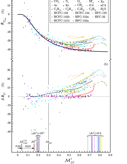
Figure 5: (Color online) lin-lin scale: a) Residuals (expressed in %) for the experimental master parachor from reference to the asymptotical master parachor calculated by Eq. (36), as a function of the master order parameter density; the full black curve corresponds to Eq. (92) (see text); b) Deviation (expressed in %) of the experimental residuals estimated in part (a), from reference to the full black curve of Eq. (92).

We have shown that the power law $\mathcal{\widetilde{Z}}_{\sigma}\left(\mathcal{M}_{\text{th}}^{*}\right)^{\pi_{a}}$ [see Eq. (36)], where $\mathcal{M}_{\text{th}}^{*}$ can be estimated as a modified theoretical function of $\mathcal{T}^{*}<0$, provides an asymptotic scaling behavior which agrees with the available experimental results in the range $\mathcal{M}_{LV}^{*}<\mathcal{M}_{\text{PAD}}^{\left\{1f\right\}}\simeq 0.04$ (see Figs. 4a and b). In this range close to the critical point, the Ising-like universal features estimated from the massive renormalization scheme are then correctly accounted for, in conformity with a (dimensionless) fluid characterization which only uses the two scale factors $Y_{c}$ and $Z_{c}$.

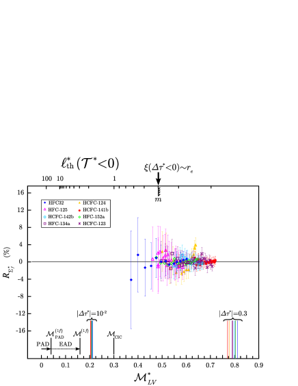
Figure 6: (Color online) lin-lin scale: Residuals (expressed in %) for the experimental master parachor of eight HFCs and HCFCs (see Refs. Okada1986 ; Okada1987 ; Higashi1992 ; Okada1995 ), from reference to the master parachor calculated by Eq. (101).

To magnify the relative master behavior at large values of $\mathcal{M}_{LV}^{*}$, i.e. beyond the preasymptotic range $\mathcal{M}_{LV}^{*}>\mathcal{M}_{\text{PAD}}^{\left\{1f\right\}}\simeq 0.04$, we have reported the (%)-residuals

$$R_{\Sigma_{\text{PAD}}^{*}}=100\left[\frac{\Sigma^{*}}{\mathcal{\widetilde{Z}}_{\sigma}\left(\mathcal{M}_{\text{th}}^{*}\right)^{\pi_{a}}}-1\right]$$ (91)

as a function of $\mathcal{M}_{LV}^{*}\equiv\mathcal{M}_{\text{th}}^{*}$ in Fig. 5a, using lin-lin scale. We have also reported the values $\mathcal{M}_{\text{PAD}}^{\left\{1f\right\}}$ [see Eq. (41)], $\mathcal{M}^{\left\{1f\right\}}$ [see Eq. (42)], and $\mathcal{M}_{\text{CIC}}$ [see Eq. (43)], which characterize the finite distances to the critical point where $\ell_{\text{th}}^{*}\simeq 40$, $\ell_{\text{th}}^{*}\simeq 3$, and $\ell_{\text{th}}^{*}\simeq 1$, respectively (as previously discussed in 2.4). This figure reveals the unambiguous non-universal nature of each fluid at large distance from the critical point, i.e., when $\ell_{\text{th}}^{*}\lesssim\frac{1}{2}$. Moreover, the observed master behavior in the extended asymptotic domain $\mathcal{M}_{\text{PAD}}^{\left\{1f\right\}}\lesssim\mathcal{M}_{LV}^{*}<\mathcal{M}^{\left\{1f\right\}}\simeq 0.16$, i.e., $40\gtrsim\ell_{\text{th}}^{*}\gtrsim 3$, needs to introduce a master correction which can reach $-(10-20)\%$ at the largest extension $\mathcal{M}^{\left\{1f\right\}}\simeq 0.16$.

To account for this correction in a quantitative manner, we have used the following convenient form,

$$R_{\Sigma_{\text{mas}}^{*}}=-100A_{\Sigma}\exp\left[-B_{\Sigma}\left(\frac{1}{\mathcal{M}_{\text{th}}^{*}}-\ln\left[\mathcal{M}_{\text{th}}^{*}\right]\right)\right]$$ (92)

which has two adjustable master parameters ($A_{\Sigma}$ and $B_{\Sigma}$) to control the following main features:

i) within the Ising-like preasymptotic domain, this function takes zero-value which preserves the Ising-like universal features contained in $\mathcal{M}_{\text{th}}^{*}\left(\left|\mathcal{T}^{*}\right|\right)$ , only characterized by $Y_{c}$ and $Z_{c}$;

ii) beyond the Ising-like preasymptotic domain, this function must provide an easy control of supplementary adjustable parameters needed to recover each real fluid behavior at large distance from the critical point.

Practically, the master values $A_{\Sigma}=0.575243$ and $B_{\Sigma}=0.302034$ of the adjustable parameters were thus obtained by optimizing the fit on the experimental %-residuals of the normal fluids Xe, Kr, N₂, and O₂, as illustrated by the corresponding black full curve in Fig. 5a. For any other selected fluid, it was then easy to estimate the related “non-universal” deviation, expressed in %, i.e., $\delta R_{\Sigma^{*}}=100\left[\frac{R_{\Sigma_{\text{PAD}}^{*}}}{R_{\Sigma_{\text{mas}}^{*}}}-1\right]$, as shown in Fig. 5b. We observe that, the larger the value of the renormalized order parameter density, the more the fluid behaviors differentiate and the “larger” is the deviation (in amplitude and shape) from the master crossover behavior.

Fluid	$\varphi_{e}$	$S_{0,e}$	$\beta_{e}$	$B_{e}$	$\phi_{e}$	$\sigma_{0,e}$	$\pi_{a,e}$	$\Sigma_{0,e}$	$p_{f}$	$\Sigma_{f}^{*}$
		($mm^{2}$)				($mN\,m^{-1}$)		($mN\,m^{-1}$)
HFC-32	$0.935257$	$8.88119$	$0.330003$	$2.00938$	$1.26526$	$74.0278$	$3.833665$	$5.098332$	$1,75798$	$0,145884$
HFC-125	$0.9220591$	$4.985323$	$0.3182363$	$1.897228$	$1.240295$	$52.68437$	$3,896303$	$4.342498$	$5,014323$	$0,5406810$
HFC-134a	$0.8912903$	$5.830025$	$0.3115459$	$1.876448$	$1.202836$	$50.00357$	$3.859691$	$4.843207$	$1,087740$	$0,1497465$
HFC-152a	$0.904293$	$8.575218$	$0.316563$	$1.903243$	$1.220856$	$59.05906$	$3.856065$	$4.936506$	$1,043043$	$0,1492084$
HCFC-123	$0.9785701$	$6.054669$	$0.2967141$	$1.795946$	$1.275284$	$59.07641$	$4.298258$	$4.769023$	$2,923514$	$0,4197302$
HCFC-124	$0.9073108$	$5.270590$	$0.289472$	$1.768259$	$1.196783$	$51.72997$	$4,116035$	$4.912059$	$2,015201$	$0,3815439$
HCFC-141b	$0.9246801$	$7.477146$	$0.3048532$	$1.794835$	$1.229533$	$60.5395$	$4,033156$	$5.721538$	$1,678934$	$0,1952588$
HCFC-142b	$0.9173884$	$7.002359$	$0.3062231$	$1.903243$	$1.223612$	$55.82877$	$3.996039$	$5.114294$	$1,939504$	$0,2315527$

Table 3: Fitting values of the effective exponent-amplitude parameters for power law description by Eqs. (93), (95), (96), (97), and (101) of experimental interfacial properties (see Refs. Okada1986 ; Okada1987 ; Higashi1992 ; Okada1995 ) of eight HFCs and HCFCs.

The theoretical estimation of these fluid differences, for example in the range of the VLE line which includes the temperature value $T=0.7\,T_{c}$ where the acentric factor is defined, is out of the present understanding of any fluid theory. However, we can use a practical approach detailed in Ref. LeNeindre2007 , where the main objective is to recover consistency with the usual description of the surface tension at large distance from the critical point by the equation

$$\sigma=\sigma_{0,e}\left|\Delta\tau^{*}\right|^{\phi_{e}}$$ (93)

In the above effective power law, $\sigma_{0,e}$ and $\phi_{e}$ are the two adjustable parameters which characterize each one-component fluid. Indeed, the noticeable result is a quasi-constant value of $\phi_{e}$ which is found in the $1.2-1.3$ range for most of the fluids, but which significantly differs from the mean-field value $\phi_{MF}=\frac{3}{2}$, as mentioned in our introduction. In this Appendix, we limit the analysis to the $S_{g}$ and $\sigma$ data which are tabulated as a function of $T$ data in Refs. Higashi1992 ; Okada1995 , for eight HCFCs and HFCs listed in Table 1 (for the complete study see Ref. LeNeindre2007 ). As in the large number of experimental works related to the determination of the surface tension, only the squared capillary length data were effectively measured from differential capillary rise method (DCRM), as a function of temperature. Then the surface tension data have been calculated using Eq. (6), where the density difference $\rho_{L}-\rho_{V}$ was estimated from published ancillary equations for the liquid density and vapor density, along the VLE line. Therefore, introducing the critical temperature $T_{c}$ and the critical density $\rho_{c}$ of each selected fluid given in Table, we can re-calculate the $\Delta\rho_{LV}^{*}$ data at each tabulated value of $T_{c}-T$, using thus the equation

$$\Delta\rho_{LV}^{*}=\frac{\sigma}{g\rho_{c}S_{g}}$$ (94)

where $g=9,80665\,\text{m}\text{s}^{-2}$ is the Earth’s gravitational acceleration.

We have fitted the tabulated $\sigma$ data, using Eq. (93). In addition we have also fitted the tabulated $S_{g}$ and recalculated $\Delta\rho_{LV}^{*}$ data, using the following equations

$$S_{g}=S_{0,e}\left|\Delta\tau^{*}\right|^{\varphi_{e}}$$ (95)

$$\Delta\rho_{LV}^{*}=B_{e}\left|\Delta\tau^{*}\right|^{\beta_{e}}$$ (96)

Thus, we have checked the consistency of the above results, by fitting the tabulated $\sigma$ data as a function of the recalculated $\Delta\rho_{LV}^{*}$ data, at the same tabulated $T_{c}-T$ data, using the following “parachor” equation

$$\sigma=\Sigma_{0,e}\left(\Delta\rho_{LV}^{*}\right)^{\pi_{a,e}}$$ (97)

The adjustable values of $\sigma_{0,e}$, $\phi_{e}$, $S_{0,e}$, $\varphi_{e}$, $B_{e}$, $\beta_{e}$, $\Sigma_{0,e}$, and $\pi_{a,e}$, are reported in Table 3 and permit to validate the interrelations $\beta_{e}=\phi_{e}-\varphi_{e}$, $\pi_{a,e}=\left(1-\frac{\varphi_{e}}{\phi_{e}}\right)^{-1}$, $B_{e}=\frac{\sigma_{0,e}}{g\rho_{c}S_{0,e}}$, and $\Sigma_{0,e}=\frac{g\rho_{c}S_{0,e}}{\left(B_{e}\right)^{\frac{\varphi_{e}}{\beta_{e}}}}$. As a conclusive remark, it appears that the Eqs. (93) and (97) are explicit results due to the initial use of “power laws” [see Eqs. (95) and (96)] to fit the “measured” $S_{g}$ data and $\Delta\rho_{LV}^{*}$ data, respectively, in the same restricted temperature range. The interfacial properties $S_{g}$, $\rho_{L}-\rho_{V}$, and $\sigma$, of each fluid are then characterized by two amplitude-exponent pairs, i.e., four adjustable parameters (in addition to the needed critical parameters which characterize the liquid-vapor critical point). Moreover, in such a self-consistent result of the fitting, the relative error-bar on the surface tension data can then be readily approximated by the sum of the relative error-bars on the squared capillary length and coexisting relative density measurements (thus including the relative uncertainty on the $\rho_{c}$ value, generally of the order of $1\%$).

In the next step, at each tabulated temperature, we have estimated:

1) the renormalized surface tension

$$\Sigma_{\text{tab}}^{*}=\left(\alpha_{c}\right)^{d-1}\beta_{c}\sigma$$ (98)

using the tabulated $\sigma$ data, and

2) the master surface tension

$$\begin{array}[]{cl}\Sigma_{\text{mas}}^{*}&=\mathcal{\widetilde{Z}}_{\sigma}\left[\left(Z_{c}\right)^{\frac{1}{2}}\Delta\rho_{LV}^{*}\right]^{\pi_{a}}\left\{1-\right.\\ &\left.A_{\Sigma}\exp\left[-B_{\Sigma}\left(\frac{1}{\left(Z_{c}\right)^{\frac{1}{2}}\Delta\rho_{LV}^{*}}-\ln\left[\left(Z_{c}\right)^{\frac{1}{2}}\Delta\rho_{LV}^{*}\right]\right)\right]\right\}\end{array}$$ (99)

using the recalculated $\Delta\rho_{LV}^{*}$ data. The %-deviations $\delta R_{\Sigma_{\text{mas}}}=100\left[\frac{\Sigma_{\text{tab}}^{*}}{\Sigma_{\text{mas}}^{*}}-1\right]$ at each value $\mathcal{M}_{LV}^{*}=\left(Z_{c}\right)^{\frac{1}{2}}\Delta\rho_{LV}^{*}$, have been fitted using the following power law

$$\delta R_{\Sigma_{\text{mas}}}=100\Sigma_{f}^{*}\left(\mathcal{M}_{LV}^{*}\right)^{p_{f}}$$ (100)

where $\Sigma_{f}^{*}$ and $p_{f}$ are two adjustable parameters, given in Table 3. As a final result, the parachor correlation now reads

$$\begin{array}[]{cl}\Sigma^{*}=&\mathcal{\widetilde{Z}}_{\sigma}\left(\mathcal{M}_{LV}^{*}\right)^{\frac{\beta}{\phi}}\\ &\left[1-A_{\Sigma}\exp\left[-B_{\Sigma}\left(\frac{1}{\mathcal{M}_{LV}^{*}}-\ln\left[\mathcal{M}_{LV}^{*}\right]\right)\right]\right.\\ &\left.+\Sigma_{f}^{*}\left(\mathcal{M}_{LV}^{*}\right)^{p_{f}}\right]\end{array}$$ (101)

where the “confluent” correction to the leading term contains two parts: i) a master contribution which is the same for all the pure fluids; ii) a non-universal contribution which is characterized by the exponent-amplitude pair $p_{f};\Sigma_{f}$ for each pure fluid. Figure 6 gives the corresponding residuals $R_{\Sigma_{f}^{*}}=100\left[\frac{\Sigma_{\text{tab}}^{*}}{\Sigma^{*}}-1\right]$ over the temperature range of the VLE line covered by the capillary rise measurements. In this figure, we have also reported each error-bar contribution of the experimental accuracy of $\pm 0.2\,\text{mN}\,\text{m}^{-1}$ claimed by the authors (ignoring the corresponding contribution of the claimed accuracy ($\pm 20\,\text{mK}$) on temperature measurements).

We conclude that the above practical approach based on the correct master description of the asymptotic Ising-like domain for the one-component fluid subclass, provides an easy control of the adjustable parameters needed to recover the experimental behavior at large distance from the critical temperature.

References

- (1) see for example, B. E. Poling, J. M. Prausnitz, and J. P. O’Connell, The properties of gases and liquids, 5th edition (McGraw Hill, New York, 2001).
- (2) see for example, J. S. Rowlinson and B. Widom, Molecular Theory of Capillarity (Clarendon, Oxford, 1984).
- (3) see for example, H.W. Xiang, Corresponding States Principle and Practice: Thermodynamics, Transport and Surface Properties of fluids (Elsevier, New York, 2005).
- (4) D. B. Macleod, Trans. Faraday Soc. 19, 38 (1923).
- (5) D. Broseta, Y. Melean, and C. Miqueu, Fluid Phase Equilib. 233, 86 (2005).
- (6) Guggenheim, J. Chem. Phys. 13, 253 (1945).
- (7) A. Anderko, in Equations of State for Fluids and Fluids Mixtures, edited by J. V. Sengers, R. F. Kayser, C. J. Peters, and H. J. White, Jr. (Elsevier, Amsterdam, 2000), Part I, pp. 75-126.
- (8) J. O. Hirschfelder, C. F. Curtiss, and R. B. Bird, Molecular Theory of Gases and Liquids (corrected edition), (Wiley, New York, 1964).
- (9) J. S. Rowlinson, Liquids and Liquid mixtures (Butterworths, London, 1971).
- (10) J. P. Hansen and I. R. McDonald, Theory of Simple Liquids, 2nd edition (Academic Press, London, 1986).
- (11) J. F. Ely and I. M. F. Marrucho, in Equations of State for Fluids and Fluids Mixtures, edited by J. V. Sengers, R. F. Kayser, C. J. Peters, and H. J. White, Jr. (Elsevier, Amsterdam, 2000), Part I, pp. 289-320.
- (12) G. C. Maitland, M. Rigby, E. B. Smith, and W. A. Wakeham, Intermolecular Forces, (Clarendon, Oxford, 1981).
- (13) J. D. van der Waals, Over de Continuiteit van den Gas- en Vloeistoftoestand, Ed. Sitjthoff, Leiden, 1973.
- (14) K. S. Pitzer, J. Am. Chem. Soc. 77, 3427 (1955); K. S. Pitzer, D. Z. Lippmann, R. F. Curl, C. M. Huggins, and D. E. Patersen, J. Am. Chem. Soc. 77, 3433 (1955); K. S. Pitzer and R. F. Curl, J. Am. Chem. Soc. 79, 2369 (1957); K. S. Pitzer and G.O. Hultgren, J. Am. Chem. Soc. 80, 4793 (1958); R. F. Curl and K. S. Pitzer, Ind. Eng. Chem. 50, 265 (1958).
- (15) O. Redlich and J. N. S. Kwong, Chem. Rev. 44, 233 (1949).
- (16) G. Soave, Chem. Eng. Sci. 27, 1197 (1972).
- (17) D. Y. Peng and D. B. Robinson, Ind. Eng. Chem. Fundam. 15, 59 (1976).
- (18) N. C. Patel and A. S. Teja, Chem. Eng. Sci. 37, 463 (1982).
- (19) N. C. Patel, Int. J. Thermophys. 17, 673 (1996).
- (20) L. Riedel, Chem Eng. Tech. 26, 83 (1954).
- (21) D. L. Schreiber and K. S. Pitzer, Fluid Phase Equilib. 46, 113 (1989).
- (22) C. Miqueu, D. Broseta, J. Satherley, B. Mendiboure, J. Lachaise, and A. Graciaa, Fluid Phase Equilib. 172, 169 (2000); and references therein.
- (23) R. I. Halm and T. I. Stiel, A. I. Ch. E. J. 13, 351 (1967).
- (24) S. B. Kiselev and J. F. Ely, J. Chem. Phys. 119, 8645 (2003).
- (25) V. L. Ginzburg, Sov. Phys. Solid State 2, 1824 (1960).
- (26) Y. Garrabos, Thesis, University of Paris VI, 1982.
- (27) Y. Garrabos, J. Phys. (Paris) 46, 281 (1985) [for an english version see cond-mat/0512347].
- (28) Y. Garrabos, J. Phys. (Paris) 47, 197 (1986).
- (29) Y. Garrabos, B. Le Neindre, R. Wunenburger, C. Lecoutre-Chabot, and D. Beysens, Int. J. Thermophys. 23, 997 (2002).
- (30) Y. Garrabos, Phys. Rev. E 74, 056110 (2006).
- (31) V. Privman, P. C. Hohenberg, A. Aharony, in Phase Transitions, Vol. 14 (Academic Press, 1991), Chap.1; and references therein.
- (32) see for example, J. Zinn-Justin, Quantum Field Theory and Critical Phenomena, 4th ed (Oxford University Press, 2002).
- (33) C. Bagnuls and C. Bervillier, Phys. Rev. E 65, 066132 (2002).
- (34) Y. Garrabos and C. Bervillier, Phys. Rev. E 74, 021113 (2006).
- (35) Y. Garrabos, C. Lecoutre, F. Palencia, B. LeNeindre, and C. Erkey, preprint (2006) [see cond-mat/].
- (36) C. Bagnuls and C. Bervillier, J. Phys. (France) - Lettres 45, L-95 (1984).
- (37) C. Bagnuls, C. Bervillier, and Y. Garrabos, J. Phys. (France)- Lettres 45, L-127 (1984).
- (38) A. E. van Giessen and B. Widom, Fluid Phase Equilib. 164, 1 (1999).
- (39) C. Miqueu, J. Satherley, B. Mendiboure, J. Lachaise, A. Graciaa, Fluid Phase Equilib. 180, 327 (2001).
- (40) see for example, M. A. Anisimov and J. V. Sengers, in Equations of State for Fluids and Fluids Mixtures, edited by J. V. Sengers, R. F. Kayser, C. J. Peters, and H. J. White, Jr. (Elsevier, Amsterdam, 2000), Part I, pp. 381-434.
- (41) B. Widom, J. Chem. Phys. 43, 3892 (1965); 43, 3898 (1965).
- (42) S. Fisk and B. Widom, J. Chem. Phys. 50, 3219 (1969).
- (43) R. Guida and J. Zinn-Justin, J. Phys. A: Math. Gen. 31, 8103 (1998).
- (44) B. Widom, J. Phys. Chem. 100, 13190 (1996).
- (45) F. J. Wegner, Phys. Rev. B 5, 4529 (1972).
- (46) J.M.H. Levelt-Sengers and J. V. Sengers, in Perspectives in Statistical Physics, edited by H. J. Ravech (North-Holland Pub. Comp., Amsterdam, 1981) pp. 241-271.
- (47) C. Bagnuls and C. Bervillier, Phys. Rev. B 32, 7209 (1985).
- (48) C. Bagnuls, C. Bervillier, D. I. Meiron, and B.G. Nickel, Phys. Rev. B 35, 3585 (1987); 65, 149901(E) (2002).
- (49) S. Sugden, J. Chem. Soc. 168, 38 (1924).
- (50) S. Sugden, J. Chem. Soc. Trans. 119, 1483-1492 (1921).
- (51) Y. Garrabos, F. Palencia, C. Lecoutre, D. Broseta, B. LeNeindre, and C. Erkey, Phys. Rev. E 75, 061112 (2007).
- (52) H. L. Gielen, O. B. Verbeke, and J. Thoen, J. Chem. Phys. 81, 6154 (1984).
- (53) M. R. Moldover, Phys. Rev. A 31, 1022 (1985).
- (54) is the (Fisher) exponent associated to the universal feature of the correlation function at the exact critical point (; ), while is the exponent associated to the universal feature of the ordering field along the critical isotherm (; ).
- (55) B. Le Neindre and Y. Garrabos, Fluid Phase Equilib. 198, 165 (2002).
- (56) M. Okada, T. Ohtake, M. Hattori, and K. Watanabe, in Proceedings of the Seventh Japan Symposium on Thermophysical Properties, 1986, pp. 183-186.
- (57) M. Okada, T. Ohtake, M. Hattori, and K. Watanabe, in Proceedings of the Eighth Japan Symposium on Thermophysical Properties, 1987, pp. 113-116.
- (58) Y. Higashi, T. Ikeda, K. Kuwana, and M. Okada, Trans. J. A. R. 9, 191 (1992).
- (59) M. Okada and Y. Higashi, Int. J. Thermophys. 16, 791 (1995).
- (60) M. R. Moldover and J. C. Rainwater, J. Chem. Phys. 88, 7772 (1988).
- (61) H. B. Chae, J. W. Schmidt, and M. R. Moldover, J. Chem. Eng. Data 35, 6 (1990).
- (62) K. G. Wilson, Phys. Rev. B 4, 3174 (1971); K.G. Wilson and J. K. Kogut, Phys. Rep. C 12, 75 (1974).
- (63) D. Stansfield, Proc. Phys. Soc. London, 72, 854 (1958).
- (64) A. J. Leadbetter and H. E. Thomas, Trans. Faraday Soc. London 61, 10 (1965).
- (65) F. B. Sprow and J. M. Prausnitz, Trans. Faraday Soc. London 62, 1097-1104 (1966).
- (66) B. L. Smith, P. R. Gardner, and E. H. C. Parker, J. Chem. Phys. 47, 1148 (1967).
- (67) J. Zollweg, G. Hawkins, and G. Benedek, Phys. Rev. Lett. 27, 1182 (1971).
- (68) J. S. Herpin and J. Meunier, J. Phys. (Paris) 35, 847 (1973).
- (69) E. S. Wu and W. W. Webb, Phys. Rev. A 8, 2077 (1973).
- (70) U. Grigull and J. Straub, in Progress in Heat and Mass Transfer, edited by T. F. Irvine, Jr., W. E. Ibele, J. P. Hartnett, and R. J. Goldstein (Pergamon, New York, 1969), Vol. 2, pp. 151-162.
- (71) W. Rathjen and J. Straub, Proceedings of the 7th Symposiumon Thermophysical Properties ASME, 1977, pp. 839-850; W rme- und Stoff bertragung 14, 59 (1980).
- (72) Y. Garrabos, F. Palencia, C. Lecoutre, C. Erkey, and B. LeNeindre, Phys. Rev. E 73, 026125 (2006).
- (73) see for example, S.-Y. Zinn and M. E. Fisher, Physica A 226, 168 (1996).
- (74) Y. Garrabos, Preprint 2005 [see cond-mat/0512408].
- (75) B. LeNeindre and Y. Garrabos, in preparation.