The Kinematics of Manipulators Built From Closed Planar Mechanisms

Abstract

The paper discusses the kinematics of manipulators builts of planar closed kinematic chains. A special kinematic scheme is extracted from the array of these mechanisms that looks the most promising for the creation of different types of robotic manipulators. The structural features of this manipulator determine a number of its original properties that essentially simplify its control. These features allow the main control problems to be effectively overcome by application of the simple kinematic problems. The workspace and singular configurations of a basic planar manipulator are studied. By using a graphic simulation method, motions of the designed mechanism are examined. A prototype of this mechanism was implemented to verify the proposed approach.

KEY WORDS : Kinematics, Manipulator, Closed Planar Mechanism, Singularity, Workspace

1 Introduction

Closed kinematic chains are promising building blocks to build novel and effective parallel manipulators. There are two principal directions in the synthesis of these machines. The first is based on the use of platform spatial manipulators. This approach has its origin in the Stewart-Gough platform [1] and has been studied extensively [2]. It is well known that platform manipulators are characterized by high stiffness and accuracy, but, at the same time, have a restricted workspace and pose some control difficulties because of their quite complicated direct kinematics.

Therefore, another direction is now under development, based on the use of closed planar kinematic chains as building blocks of spatial robots. We claim that this very promising approach has not yet been fully exploited.

The simplest example of a basic planar manipulator of this type, shown in Figure 1, has motivated intensive research (e.g., [3]). This mechanism is based on the use of a dyad, that is, a planar group of the second class, links 1 and 2, according to the classification of Assur-Artobolevskii [4].

Rotation about a vertical axis provides this mechanism with three-degree-of-freedom (dof) motion capabilities. The advantages of the mechanism are enhanced stiffness and driving motor placement on the base (joints $A$ and $B$), both advantages being common properties of parallel manipulators. However, only manipulators built on planar closed chains have the advantages of rather simple kinematics and a relatively large workspace. In fact, the layout of Fig. 1 was so effective that it has been the first closed kinematic chain used in one of the versions of the German “Kuka” industrial robot.

A disadvantage of the scheme shown in Fig. 1 is its somewhat restricted workspace, determined by the distance between the base joints $A$ and $B$. Based on kinematic considerations, this distance may be chosen to be near zero, as was practically implemented in the design of the “Kuka” robot.

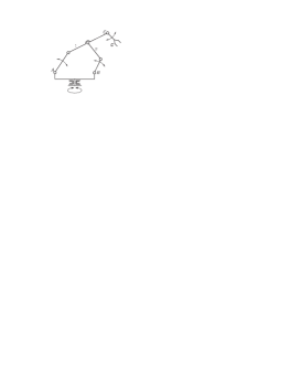
Fig. 1: Three-dof manipulator based on planar mechanism of second class

Another feature of the basic mechanism (Fig. 1) is that if we need to control the orientation of the gripper $G$, it is usually necessary to mount an additional actuator in the joint $C$ of the moving link 1.

A solution that allows one to solve this problem without putting a motor on the moving link involves the third class group [4] as a basic kinematic chain (Fig. 2).

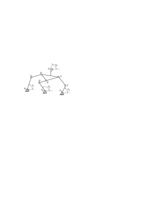
Fig. 2: Planar manipulator based on the mechanism of third class

This mechanism has gained its reputation thanks to Hunt (e.g., [2]) and the following publications [6, 7]. It is, in fact, very important and interesting because it serves as a link between the two above-mentioned approaches in organization of robot platform mechanisms. Indeed, it is possible to pass from the planar closed mechanism (Fig. 2) to the platform spatial manipulator by changing the revolute joints (points $D,E$ and $F$) by spherical joints and by removing the dyads $O_{1}A,AD;O_{2}B,BE;$ and $O_{3}C,CF$ onto different planes.

The third-class mechanisms are the most promising to organize prospective spatial industrial robots, as demonstrated in a patent [8]. In this design, the moving platform, link $DEF$, of the Assur group (Fig. 2) was attached to the prismatic kinematic pair directed orthogonally to the plane of group location.

Third-class mechanisms have good prospects because of a quite simple kinematics. In this connection, a number of investigations were carried out to determine theirs workspace, singular configurations and other characteristics ([6, 7]). Currently, some propositions have been made in which linear actuators of robotic mechanisms are used as input links [9].

This paper develops this approach in creating closed structural schemes for platform robot mechanisms. A special variation of the discussed mechanisms with a linear platform link [10] and other peculiarities, ensuring a high level of solution of the manipulation tasks to be performed, is proposed for development, their design and control features being analyzed in this paper.

2 Structure of the Three-DOF Manipulator

The design of a robot based on third-class chains becomes practical when the mechanism is specially constructed as discussed below. This section considers a special kind of the basic third-class planar chain, shown in the mechanism of Fig. 3.

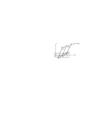
Fig. 3: A scheme of the proposed base planar manipulator

Specifically, its moving platform $C_{1}G$ carries three collinear joints, and its actuated joints are prismatic. The actuators of these joints are placed in different parallel planes. The collinear form of the platform element prevents collisions among the links. This base manipulator performs spatial motions by means of additional joints with suitably-oriented axes. Such a structure leads to a considerable simplification of the control as compared with the initial mechanism of Fig. 2.

3 Kinematics

The actuated joint variables are $\rho_{1}=||A_{1}B_{1}||$, $\rho_{2}=||A_{2}B_{2}||$ and $\rho_{3}=||A_{3}B_{3}||$ while the Cartesian variables are the $(x_{G},y_{G},\theta_{G})$ coordinates of the end-effector (Fig. 3). Lengths $L_{11}=||B_{1}C_{1}||$, $L_{22}=||B_{2}C_{2}||$, $L_{33}=||B_{3}C_{3}||$, $L_{1G}=||C_{1}G||$, $L_{2G}=||C_{1}G||$ and $L_{3G}=||C_{1}G||$ define the geometry of this manipulator entirely.

The velocity $\dot{\bf{g}}$ of the point $G$ can be obtained in three different forms, depending on the direction in which the loop is traversed [11, 12], namely:

$$\dot{{\bf{g}}}=\dot{{\bf{b}}}_{1}+\dot{\alpha_{1}}{\bf{E}}({\bf{c}}_{1}-{\bf{b}}_{1})+\dot{\theta_{G}}{\bf{E}}({\bf{g}}-{\bf{c}}_{1})$$ (1)

$$\dot{{\bf{g}}}=\dot{{\bf{b}}}_{2}+\dot{\alpha_{2}}{\bf{E}}({\bf{c}}_{2}-{\bf{b}}_{2})+\dot{\theta_{G}}{\bf{E}}({\bf{g}}-{\bf{c}}_{2})$$ (2)

$$\dot{{\bf{g}}}=\dot{{\bf{b}}}_{3}+\dot{\alpha_{3}}{\bf{E}}({\bf{c}}_{3}-{\bf{b}}_{3})+\dot{\theta_{G}}{\bf{E}}({\bf{g}}-{\bf{c}}_{3})$$ (3)

with matrix ${\bf E}$ defined as

$${\bf E}=\left[\begin{array}[]{cc}0&-1\\ 1&0\end{array}\right]$$

and ${\bf{b}}_{i}$ and ${\bf{c}}_{i}$ denoting the position vectors in the frame $x$-$y$ of Fig. 3 of the points $B_{i}$ and $C_{i}$ respectively, for $i=1,2,3$.

Furthermore, note that vectors $\dot{{\bf{b}}}_{i}$ are given by

$$\dot{{\bf{b}}}_{i}=\dot{\rho}_{i}\frac{{\mbox{\boldmath${\rho}$\unboldmath}_{i}}}{||{\bf{\rho}}_{i}||}.$$ (4)

We would like to eliminate the three idle joint rates $\dot{\alpha}_{1}$, $\dot{\alpha}_{2}$ and $\dot{\alpha}_{3}$ from eqs.(1-2-3), which we do upon dot-multiplying their two sides by ${\bf{c}}_{i}-{\bf{b}}_{i}$, thus obtaining

$$({\bf{c}}_{1}-{\bf{b}}_{1})^{T}\dot{{\bf{g}}}=({\bf{c}}_{1}-{\bf{b}}_{1})^{T}\dot{\rho}_{1}\frac{{\mbox{\boldmath${\rho}$\unboldmath}_{2}}}{||{\bf{\rho}}_{1}||}+({\bf{c}}_{1}-{\bf{b}}_{1})^{T}\dot{\theta_{G}}{\bf{E}}({\bf{g}}-{\bf{c}}_{1}),$$ (5)

$$({\bf{c}}_{2}-{\bf{b}}_{2})^{T}\dot{{\bf{g}}}=({\bf{c}}_{2}-{\bf{b}}_{2})^{T}\dot{\rho}_{2}\frac{{\mbox{\boldmath${\rho}$\unboldmath}_{2}}}{||{\bf{\rho}}_{2}||}+({\bf{c}}_{2}-{\bf{b}}_{2})^{T}\dot{\theta_{G}}{\bf{E}}({\bf{g}}-{\bf{c}}_{2}),$$ (6)

$$({\bf{c}}_{3}-{\bf{b}}_{3})^{T}\dot{{\bf{g}}}=({\bf{c}}_{3}-{\bf{b}}_{3})^{T}\dot{\rho}_{3}\frac{{\mbox{\boldmath${\rho}$\unboldmath}_{3}}}{||{\bf{\rho}}_{3}||}+({\bf{c}}_{3}-{\bf{b}}_{3})^{T}\dot{\theta_{G}}{\bf{E}}({\bf{g}}-{\bf{c}}_{3}).$$ (7)

Equations (5-6-7) can now be cast in vector form:

$${\bf A}\dot{{\bf{p}}}={\bf B\dot{\bf q}}$$ (8)

with $\dot{\bf q}$ defined as the vector of actuated joint rates, of components $\dot{\rho}_{1}$, $\dot{\rho}_{2}$ and $\dot{\rho}_{3}$ and $\dot{{\bf{p}}}$ defined as the planar twist vector of components $\dot{x_{G}}$, $\dot{y_{G}}$ and $\dot{\theta_{G}}$. Moreover ${\bf A}$ and B are, respectively, the direct-kinematics and the inverse-kinematics matrices of the manipulator, defined as

$${\bf A}=\left[\begin{array}[]{cc}({\bf{c}}_{1}-{\bf{b}}_{1})^{T}&({\bf{c}}_{1}-{\bf{b}}_{1})^{T}{\bf{E}}({\bf{g}}-{\bf{c}}_{1})\\ ({\bf{c}}_{2}-{\bf{b}}_{2})^{T}&({\bf{c}}_{2}-{\bf{b}}_{2})^{T}{\bf{E}}({\bf{g}}-{\bf{c}}_{2})\\ ({\bf{c}}_{3}-{\bf{b}}_{3})^{T}&({\bf{c}}_{3}-{\bf{b}}_{3})^{T}{\bf{E}}({\bf{g}}-{\bf{c}}_{3})\end{array}\right]$$ (9)

and

$${\bf B}\!\!\!\!=\!\!\!\!\left[\begin{array}[]{ccc}\!\!({\bf{c}}_{1}\!-\!{\bf{b}}_{1})^{T}{\mbox{\boldmath${\rho}$\unboldmath}_{1}}/||{\bf{\rho}}_{1}||\!\!\!\!\!&0&0\\ 0&\!\!\!\!\!\!\!\!({\bf{c}}_{2}\!-\!{\bf{b}}_{2})^{T}{\mbox{\boldmath${\rho}$\unboldmath}_{2}}/||{\bf{\rho}}_{2}||\!\!\!\!\!\!\!\!&0\\ 0&0&\!\!\!\!\!({\bf{c}}_{3}\!-\!{\bf{b}}_{3})^{T}{\mbox{\boldmath${\rho}$\unboldmath}_{3}}/||{\bf{\rho}}_{3}||\!\!\end{array}\right]$$ (10)

3.1 Control of Simple Motions

An original property of the manipulator under study is its ability to carry out simple motions either without performing any preliminary calculations, or by using some simple kinematic relationships [13]. We summarize below these results: Horizontal Translation In this case, $\dot{y}_{G}=0$, $\dot{\theta}_{G}=0$ and $\dot{x}_{G}$ is arbitrary. The solution leads to a simultaneous motion of all actuators with the same velocities, that is, $V_{1}=V_{2}=V_{3}=V_{G}$, while $V_{G}$ is the prescribed gripper velocity. Vertical Translation In this case, $\dot{x}_{G}=0$, $\dot{\theta}_{G}=0$, and $\dot{y}_{G}$ is arbitrary. Thus,

$$\dot{\rho_{i}}=V_{G}\tan\alpha_{i},\;i=1,2,3.$$ (11)

while $V_{G}$ is the prescribed gripper velocity.

In the general case, in order to obtain the vertical end-effector velocity, it is necessary to use the simple expressions (11) for calculations and to measure angles $\alpha_{i}$, for $i=1,2,3$. Gripper Rotation Here, $\dot{\theta}_{G}$ is arbitrary and $\dot{x}_{G}=\dot{y}_{G}=0$, thus obtaining

$$V_{i}=L_{iG}\dot{\theta}_{G}\frac{\sin(\alpha_{i}-\theta_{G})}{\cos\alpha_{i}},\;i=1,2,3.$$ (12)

It is apparent that the values $\alpha_{i}$ and $\theta_{G}$ have to be measured. The $\alpha_{i}$ values were already used for other calculations, but angle $\theta_{G}$ has to be measured only for this problem. This can be done by measuring the angle of rotation of one of the $C_{i}$ joints (Fig. 3), with the ensuring calculation of the angle $\theta_{G}$:

$$\theta_{G}=\beta+\alpha_{1}-180^{\circ}.$$

Thereafter, a pure rotation of the gripper can be implemented, which cannot be realized for any other design of spatial platform manipulators.

3.2 Singular Configurations of the Proposed Manipulator

A singularity occurs whenever A or B in (9) vanishes. Three types of singularities exist [6]:

$${\rm det}({\bf{A}}) = 0{\rm~{}or}$$

$${\rm det}({\bf{B}}) = 0{\rm~{}or}$$

$${\rm det}({\bf{A}}) = 0\quad{\rm and}\quad{\rm det}({\bf{B}})=0.$$

Parallel singularities occur when the determinant of the direct kinematics matrix A vanishes. The corresponding singular configurations are located inside the workspace. They are particularly undesirable because the manipulator cannot resist any force and control is lost.

For the manipulator study, there are two types of parallel singularities.

The first type is reached whenever the lines $B_{i}C_{i}$ intersect (Fig. 4). In such configurations, the manipulator cannot resist a wrench applies at the intersecting point.

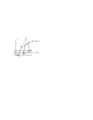
Fig. 4: A parallel singularity

The second type is reached whenever the lines $B_{i}C_{i}$ are parallel (Fig. 5). That is when $({\bf{c}}_{1}-{\bf{b}}_{1})\times({\bf{c}}_{2}-{\bf{b}}_{2})={\bf{0}}$ and $({\bf{c}}_{1}-{\bf{b}}_{1})\times({\bf{c}}_{3}-{\bf{b}}_{3})={\bf{0}}$.

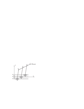
Fig. 5: A parallel singularity

Serial singularities occur when the determinant of the inverse kinematics matrix B vanishes. When the manipulator is in such a singularity, there is a direction along which no Cartesian velocity can be produced.

For the manipulator at hand, serial singularities occur whenever at least one of the lines $A_{i}B_{i}$ is perpendicular to $B_{i}C_{i}$, i.e $({\bf c_{i}}-{\bf b_{i}})^{T}\mbox{\boldmath${\rho_{i}}$\unboldmath}/||{\bf{\rho}}_{i}||=0$, for $i=1,2,3$ (Fig. 6). These singularities yield the boundary of the Cartesian workspace.

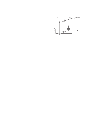
Fig. 6: A serial singularity

4 Manipulator Workspace

It is important to determine the manipulator workspace to exactly match its working zone. Generally, the planar manipulator workspace is limited by a rectangle with height $h$ and width $w$. The value $h$ may be determined as

$$h={\rm min}\{L_{1G}+L_{11},L_{2G}+L_{22},L_{3G}+L_{33}\},$$

where we refer to variables defined in Section 3 and Fig. 3. The value of $w$ is estimated as $w=2h+L$, where $L$ is the length of the actuator strokes.

To study manipulator workspace properties, a special numerical procedure has been developed. According to this procedure, the space of the above-mentioned rectangle was divided with a certain resolution into a number of points. For each of these points, a test was then done whether the mechanism with a corresponding set of parameters exists with a manipulator end-effector $G$ position at this point. If this condition is satisfied at least for one orientation of the output link or not satisfied for all orientations of the output link, a passage to the next point of the rectangle is performed. This numerical procedure gives us the possibility to obtain not only an envelope of the manipulator working zone but also configurations of its dead points.

One example of these results is displayed in Fig. 7.

Fig. 7: Example of a manipulator workspace (a part above the $x$ axis) for the following set of its model parameters: $L_{11}=L_{22}=L_{33}=25.0$, $||C_{1}C_{2}||=||C_{2}C_{3}||=||C_{3}G||=5.0,L=10.0$

From this graph as well as from geometric considerations, it is obvious that the value of the stroke $L$ influences the shape of the manipulator workspace. When $L$ decreases, dead zones appear inside the manipulator envelope. This study has been conducted and corresponding results are recorded in graph form (Fig. 8).

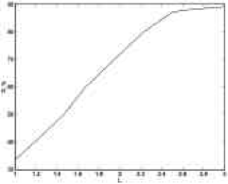
Fig. 8: The relative value $S$ of the manipulator workspace vs stroke length $L$

A study was carried out for the following set of manipulator parameters: $L_{11}=1.7,L_{22}=1.8,L_{33}=1.9;||C_{1}C_{2}||=||C_{2}C_{3}||=||C_{3}G||=1.0$; the value of $L$ was changed from 1 to 3. A characteristic of the value $S$ of the manipulator workspace was defined as a relation of the number of points, where there is at least one inverse kinematics solution, to a general quantity of the points studied in the rectangle. When studying the value $S$ dependence on the stroke length $L$, one should take into account that an increase in the stroke length will lead to an increase in the workspace. However, too long stroke value may lead to a bulky mechanism. This is why, when searching for the optimal value of the stroke, it would be worth to chose it not longer than the length allowing to exclude some dead zones inside the manipulator workspace (if there are no special requirements to manipulator performance). Then, from the graph of Fig. 8, it may be seen that the best result is obtained for $L=3$ (89.07%), but a result for the value $L=2.5$ (87.08%) is quite near to this maximum value.

Based on these data, one may conclude that this approach allows us to determine manipulator optimum parameters which lead to the design of the most versatile and compact device.

5 Simulation and Prototyping of the Proposed Manipulator

A graphic simulation of the proposed 3D manipulator based on the mechanism of Fig. 3 was performed by using an advanced robotics package on a Silicon Graphics workstation [13]. Typical positioning tasks were simulated and successive spatial motions of the robot from one location to another were tested. The kinematic structure was evaluated by animated, graphical representation of the time-varying solutions that includes built-in evaluation of trajectories to avoid collisions, and reachability. One rendering of the simulation results is shown in Fig. 9.

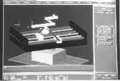
Fig. 9: Rendering of the manipulator

A prototype of the planar mechanism discussed here was also built (Fig. 10) when the first author was working at Kazakh State University (Alma-Ata, Kazakhstan, the former USSR).

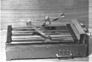
Fig. 10: Manipulator prototype

The mechanism is driven by three DC motors with on-off control. The prototype allowed, for instance, to validate issues of mechanism singularities and approaches to their avoidance.

6 Conclusions

This paper deals with closed-chain planar mechanisms with the purpose of using them for the design of 3D parallel robotic manipulators. The paper proposes some principles of spatial manipulator design via these mechanisms. A paradigm is proposed that appears to be the most promising for the design of multi-dof industrial robots. Its peculiarities are the platform link in the form of a collinear array of attachment points and actuators that are designed in the form of sliders placed in different parallel planes.

While using this mechanism as a basis for multi-dof manipulator design, the indicated structural features determine a number of its original properties that essentially simplify its control. A parallel manipulator of a practical form of this design has been previously developed, which was rather similar to one recently called the H-Robot [9]. This manipulator allows one to solve the principal control problems almost without the need to solve their inverse kinematics. In fact, the kinematic solutions are either extremely simple or do not require any calculations. For instance, the translation of the gripper along the $x$ axis (Fig. 3) may be obtained with the aid of the translation of the actuators in the required direction with equal velocities, that is, without performing any calculations. A vertical displacement of the end-effector is accomplished by moving the actuators by implementing some very simple calculations. These special features allow one to develop rather simple control algorithms for the robot.

Workspace and singular configurations were also studied for purpose of robot design. By using graphic simulations, the motions of the designed mechanism were examined. A prototype of the discussed mechanism was also built in order to test the proposed approach.

References

- [1] D.A. Stewart, “Platform with six degree of freedom,” Proceedings of the Institute of Mechanical Engineering, 66, Vol. 180, Part 1, No. 15, pp. 371-386, 1965.
- [2] K.H. Hunt, “Structural kinematics of in-parallel-actuated robot-arms,” ASME Journal of Mechanisms, Transmissions, and Automation in Design, Vol. 105, pp. 705-712, 1983.
- [3] A. Bajpai and B. Roth, “Workspace and mobility of a closed-loop manipulator,” The International Journal of Robotics Research, Vol. 5, No. 2, pp. 131-142, 1986.
- [4] I.I. Artobolevskii, Theory of Mechanisms and Machines, Nauka, Moscow, 1988 (in Russian).
- [5] G.N. Sandor and A.G. Erdman, Mechanical Design: Analysis and Synthesis, Prentice Hall, 1984.
- [6] C. Gosselin and J. Angeles, “Singularity analysis of closed loop kinematic chains,” IEEE Transactions on Robotics and Automation, Vol. 6, No. 3, pp. 281-290, 1990.
- [7] G. Pennok and D. Kassner, “The workspace of a general geometry planar three-degree-of-freedom platform-type manipulator,” ASME Journal of Mechanical Design, Vol. 115, pp. 269-276, 1993.
- [8] U.A. Djoldasbekov, M.S. Konstantinov, M.D. Markov, and L.I. Slutski, “Executing mechanism of a robot-manipulator,” USSR patent, author’s certificate # 1081919, 1983 (in Russian).
- [9] J.M. Hervé, “Design of parallel manipulators via the displacement group,” Proceedings Ninth World Congress on the Theory of Machines and Mechanisms, Vol. 3, 29 Aug. - 2 Sept., Italy, pp. 2079-2082, 1995.
- [10] J.-P. Merlet, “Singular configurations of parallel manipulators and Grassman geometry,” The International Journal of Robotics Research, Vol. 8, No. 5, pp. 45-56, 1989.
- [11] D. Chablat and Ph. Wenger, “Working modes and aspects in fully-parallel manipulator”, Proceeding IEEE International Conference on Robotics and Automation, pp. 1964-1969, May 1998.
- [12] H.R. Mohammadi Daniali, P. Zsombor-Murray, and J. Angeles, “Singular analysis of planar parallel manipulators,” Mechanism and Machine Theory, vol. 30, no. 5, pp. 665-678, 1995.
- [13] L. Slutski, “Closed plane mechanisms as a basis of parallel manipulators”. In: J. Lenarčič and V. Parenti-Castelli (eds.), Recent Advances in Robot Kinematics. Kluwer Academic Publishers, Dordrecht, pp. 441-450, 1996.