Emergence of scale-free behavior in networks from limited-horizon linking and cost trade-offs

Abstract

We study network growth from a fixed set of initially isolated nodes placed at random on the surface of a sphere. The growth mechanism we use adds edges to the network depending on strictly local gain and cost criteria. Only nodes that are not too far apart on the sphere may be considered for being joined by an edge. Given two such nodes, the joining occurs only if the gain of doing it surpasses the cost. Our model is based on a multiplicative parameter $\lambda$ that regulates, in a function of node degrees, the maximum geodesic distance that is allowed between nodes for them to be considered for joining. For $n$ nodes distributed uniformly on the sphere, and for $\lambda\sqrt{n}$ within limits that depend on cost-related parameters, we have found that our growth mechanism gives rise to power-law distributions of node degree that are invariant for constant $\lambda\sqrt{n}$. We also study connectivity- and distance-related properties of the networks.

I Introduction

Large-scale networks occurring in a variety of natural, technological, and social domains have been studied intensely in the last several years. In many cases, only superficial information is available on the topology of the network under study, so the most common approach has been to model it as a random graph Bollobás (2001) and to describe its properties statistically. Many of these properties seem to be related to the network’s degree distribution, which has then received considerable attention. In many instances of interest, including networks related to the Internet or to the WWW, the degree distribution is a power law. That is, the probability that a randomly chosen node has degree $k$ is proportional to $k^{-\tau}$, in general with $2<\tau<3$. For detailed information, we refer the reader to the papers collected in Bornholdt and Schuster (2003); Newman et al. (2006) and to Boccaletti et al. (2006).

An effort closely related to that of characterizing the degree distributions of existing networks has been to attempt to explain how a power law can emerge from the underlying mechanisms that govern network evolution. Many of the proposed explanations have been centered around the so-called Barabási-Albert model Barabási and Albert (1999); Barabási et al. (1999); Dorogovtsev et al. (2000); Krapivsky et al. (2000); Holme and Kim (2002); Bollobás and Riordan (2003); Cooper and Frieze (2003); Bollobás and Riordan (2004), which is essentially based on the mechanism, known as preferential attachment, according to which the appearance of a new edge connecting a new node to a preexisting one is dependent upon the latter node’s current degree in direct proportion. As we argued in an earlier work Barbosa et al. (2006), preferential attachment often leads to an unreasonable generative model for networks, since it makes network-growth decisions depend on global properties and also, for cases like that of computer networks, implies that node degrees are a more important growth factor than some cost or efficiency criterion. Other proposals, including our own in Barbosa et al. (2006), have relied on exclusively local properties Kumar et al. (2000); Caldarelli et al. (2002); Rosvall and Sneppen (2003).

The mechanism we suggested in Barbosa et al. (2006) promotes network growth by the addition of edges to a fixed set of nodes that, initially, are all part of a tree. At each time step, two nodes $i$ and $j$ not currently connected by an edge are randomly selected and an edge is placed between them if a gain function is found to surpass a cost function for the current network topology. The gain function seeks to reflect the shortening of distances on the graph that the new edge may cause between nodes in $i$’s neighborhood and nodes in $j$’s. The cost function refers to the cost of deploying the connection itself and also to the cost of possibly having to upgrade $i$ or $j$’s capabilities to accommodate the new connection. For selected parameter combinations, degree distributions comprising a two-tier hierarchy of power laws (one for the lower degrees, another for the higher) are seen to emerge.

One limitation of this mechanism is that any two nodes not currently connected by an edge may be selected to be the potential end nodes of a new edge. The trouble with this is not only the implausibility that comes with it in the context of computer networks, but also the limitation that is indirectly imposed on the gain functions that can be used. When $i$ and $j$ are selected, the gain function depends on the current distances between several node pairs, but all we may assume to be locally available without the need to probe the network beyond some reasonable depth are upper bounds on these distances. The results we reported in Barbosa et al. (2006) are then based on a gain function that uses such upper bounds and this is reflected as an oscillatory perturbation in the power laws.

Here we generalize our previous model by dispensing with the need of the initial spanning tree and also by attaching a geometric reference to each node. We take each node to be a point on the surface of a sphere and associate with it a maximum geodesic distance beyond which connections are forbidden. Not only does this render the model more plausible from the perspective of computer networks, it also allows our gain function to be expressed in terms of exact distances on the graph, since these are now obtainable from any node by controlled-depth incursions into the network.

If the maximum geodesic distance for node interconnection were the same for all nodes, then the graph obtained by joining all allowed pairs of nodes would be an instance of what is known as a two-dimensional random geometric graph with spherical boundary conditions Dall and Christensen (2002); Penrose (2003). Curiously, for such a graph the degree distribution is the same Poisson distribution that holds for the Erdős-Rényi classic random-graph case Erdős and Rényi (1959). As we see in the remainder of the paper, assuming degree-dependent maximum geodesic distances and deciding whether to interconnect two nodes based on the same trade-offs as in Barbosa et al. (2006) give rise to power-law degree distributions, now without the oscillations that were caused by using upper bounds on the distances on the graph. In addition to these distributions, we also study the emergence of a giant connected component and the relationship between distances on the graph and geodesic distances.

Our present work is related to the work described in Xulvi-Brunet and Sokolov (2007), where constraints similar to ours are imposed on the growing of the networks. However, the two works remain markedly distinct, since not only the constraints but also the growth criteria seem to be significantly different in the two cases. In particular, in Xulvi-Brunet and Sokolov (2007) both minimum and maximum geometric distances are taken into account (on the plane, which is where the authors assume the network lies) and, more importantly, a local version of preferential attachment is used.

II The model

We model network growth by the sequence $G^{0},G^{1},\ldots$ of undirected graphs, each on the same set of $n$ nodes, given that in $G^{0}$ all nodes are isolated (i.e., $G^{0}$ has no edges). We assume nodes to lie on the surface of a sphere of unit radius. For $i$ and $j$ any two nodes, there are two metrics of interest. One is $\delta_{ij}$, given by the geodesic distance between $i$ and $j$; the other, for $t=0,1,\ldots$, is $d^{t}_{ij}$, given by the distance between $i$ and $j$ in $G^{t}$ (i.e., the number of edges on the shortest path between $i$ and $j$ in $G^{t}$).

Let $n^{t}_{i}$ be the degree of node $i$ (its number of neighbors) in $G^{t}$ and $\rho^{t}_{i}$ the geodesic distance beyond which no node may be connected to $i$ in $G^{t}$. We use

$$\rho^{t}_{i}=\lambda\ln(e+n^{t}_{i})$$ (1)

throughout, where $\lambda$ is a parameter, indicating that $\rho^{t}_{i}=\lambda$ for isolated nodes (regardless of $t$) and that $\rho^{t}_{i}$ increases logarithmically with $n^{t}_{i}$ from then on. In order for $\rho^{t}_{i}$ to exclude no node from the possibility of being connected to $i$ for any $t$, it suffices to set $\lambda=\pi$.

For $i$ and $j$ any non-neighboring nodes of $G^{t}$, we define $N^{t}_{i}(j)$ to be the set comprising every neighbor $k$ of $i$ in $G^{t}$ for which $d^{t}_{jk}>2$. Clearly, any node in this set benefits from the addition of an edge between $i$ and $j$, in terms of acquiring a shorter path (of length $2$) to $j$. Not only this, but we also know that, if $k\in N^{t}_{i}(j)$, then

$$\max\{3,d^{t}_{ij}-1\}\leq d^{t}_{jk}\leq d^{t}_{ij}+1$$ (2)

(or else $d^{t}_{ij}$ could not be the distance between $i$ and $j$ in $G^{t}$). We also define $N^{t}_{ij}$ to be the set of all unordered pairs $(k,l)$ such that either $k$ or $l$ is a neighbor of $i$, the other node in the pair is a neighbor of $j$, and moreover $d^{t}_{kl}>3$. As before, any node pair in this set acquires a shorter path (of length $3$) between them as a result of adding an edge between $i$ and $j$. Additionally, for $(k,l)\in N^{t}_{ij}$,

$$\max\{4,d^{t}_{ij}-2\}\leq d^{t}_{kl}\leq d^{t}_{ij}+2.$$ (3)

[Note that both the inequality pair in (2) and the one in (3) define nonempty intervals, since $d^{t}_{ij}>1$.]

For $t\geq 0$, $G^{t+1}$ is obtained from $G^{t}$ by randomly selecting two nodes, say $i$ and $j$, such that $d^{t}_{ij}>1$ and adding an edge between them if the gain from doing so surpasses the cost, provided

$$\delta_{ij}\leq\min\{\rho^{t}_{i},\rho^{t}_{j}\}.$$ (4)

That is, we require not only a positive gain-cost trade-off, but also that the surface of the spherical cap centered on $i$ include $j$ and the one on $j$ include $i$ (in other words, the least connected node of the pair is the one that actually determines whether the connection is possible). If either condition does not hold, then $G^{t+1}=G^{t}$.

It is important to note that, even though by Eq. (1) the limitation on the horizon of admissible connections to a node is expected to grow (albeit weakly) with the node’s degree, no such trend exists regarding the probability that the node’s degree is in fact increased. Instead, it is only the size of the region inside which a new link to that node may be created that increases. Thus, clearly, our policy for adding new edges to the graph is not just a more local, weaker version of preferential attachment, but a wholly different concept.

The gain we use is denoted by $g^{t}_{ij}$ and gives the total number of edges by which certain paths become shorter when $i$ and $j$ become neighbors. These paths are the following: the one between $i$ and $j$, the one between each $k\in N^{t}_{i}(j)$ and $j$, the one between each $k\in N^{t}_{j}(i)$ and $i$, and finally the one between each pair $(k,l)\in N^{t}_{ij}$. We then have

$$g^{t}_{ij}=d^{t}_{ij}-1+\sum_{k\in N^{t}_{i}(j)}(d^{t}_{jk}-2)$$ (5)

$$+\sum_{k\in N^{t}_{j}(i)}(d^{t}_{ik}-2)+\sum_{(k,l)\in N^{t}_{ij}}(d^{t}_{kl}-3),$$

and it follows from our preceding discussion that

$$g^{t}_{ij}\geq 1+|N^{t}_{i}(j)|+|N^{t}_{j}(i)|+|N^{t}_{ij}|,$$ (6)

where $|X|$ denotes the number of elements of set $X$. Also, it is important to note that, by (4), $g^{t}_{ij}$ can be obtained by probing $G^{t}$ from $i$ nearly exclusively on the surface of $i$’s spherical cap (some of $j$’s neighbors may be excepted), and conversely from $j$. If nodes are distributed uniformly on the sphere’s surface, then by Eq. (1) this amounts to saying that, for fixed $\lambda$, probing $G^{t}$ from any node is expected to go no deeper than a distance on the graph that grows only logarithmically with the node’s degree.

The cost component of the trade-off is denoted by $c^{t}_{ij}$ and given exactly as in Barbosa et al. (2006), where the reader is referred to for complete details. The cost $c^{t}_{ij}$ is given simply by

$$c^{t}_{ij}=C+D[(n^{t}_{i})^{\gamma}+(n^{t}_{j})^{\gamma}],$$ (7)

where $C$ is the fixed cost of actually deploying the connection between $i$ and $j$ and the second term, weighted by the proportionality constant $D$, refers to amortizing the cost to upgrade the connection capabilities of $i$ and $j$.

III Computational results and discussion

Our results are based on computer simulations for which the parameter values needed in the cost function of Eq. (7) are $C=100$, $D=0.1$, and $\gamma=0.9$. These were the values identified in Barbosa et al. (2006) as giving rise to interesting scale-free behavior and here we use them exclusively. Each simulation is run through $t=3n^{2}$ from a randomly chosen $G^{0}$ instance, which in turn is obtained by placing the $n$ nodes on the unit-radius sphere uniformly at random. Most of the data we show are averages over at least $500$ independent runs (exceptions are the $n=2\,000$ cases with $\lambda\geq 0.4$, for which the number of runs is between $150$ and $500$).

Whenever necessary for use in the computation of the gain function of Eq. (5), distances on the current graph are obtained by searching it breadth-first from one of the two nodes involved. If $G^{t}$ is the graph in question and it has $m^{t}$ edges, then completing such a search requires $O(m^{t})$ time in the worst case Cormen et al. (2001). As we mentioned earlier, however, in our present case the search need not run over all of $G^{t}$. In fact, all necessary distances are expected to be found without the search proceeding any deeper in $G^{t}$ than a number of edges that depends only on $\lambda$ and a slow-growing function of node degrees, since nodes are distributed uniformly on the sphere.

Figures 1–3 show the final connectivity properties of the graph as a function of $\lambda$ (insets). While for very small $\lambda$ nearly every node is a connected component by itself, increasing the value of $\lambda$ eventually gives rise to the giant connected component, which encompasses practically all nodes. Characterizing the sharp transition that takes place between the two extremes is facilitated by a rescaling of the $\lambda$ parameter. For relatively small $\lambda$, the surface area of the spherical cap centered at node $i$ can be approximated by the area of the circle of radius $\rho^{t}_{i}$ centered at $i$. Using this approximation, and by Eq. (1), keeping $\lambda\sqrt{n}$ fixed as both $\lambda$ and $n$ vary implies that the expected number of nodes on the spherical cap remains fixed as well, provided nodes are uniformly distributed on the sphere. Rescaled plots for the connectivity-related quantities appear in the main plot sets of Figs. 1–3, indicating that the sudden rise of the giant connected component occurs at $\lambda\sqrt{n}\approx 3$.

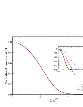
Figure 1: (Color online) Normalized number of connected components (CC) as a function of $\lambda$ (inset) and $\lambda\sqrt{n}$.

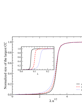
Figure 2: (Color online) Normalized size of the largest connected component (CC) as a function of $\lambda$ (inset) and $\lambda\sqrt{n}$.

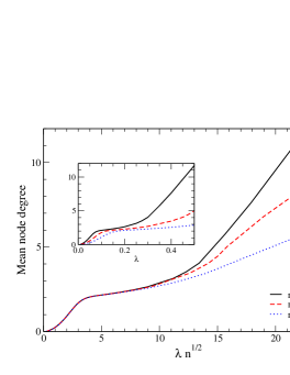
Figure 3: (Color online) Mean node degree as a function of $\lambda$ (inset) and $\lambda\sqrt{n}$.

The mean node degree increases steadily toward the values above $2$ that correspond to the presence of the giant connected component Molloy and Reed (1995); Newman et al. (2001), which already holds for values of $\lambda\sqrt{n}$ around $4$. Above this value, though, it seems that the existence of this component tends to discourage the creation of any significant number of additional edges for a relatively long stretch. As shown in Fig. 3, only for values larger than about $11$ are the gain-cost trade-offs once again effective, allowing for the sustained addition of further edges. It is curious to observe that the rescaling to $\lambda\sqrt{n}$ breaks down past this value, since the mean node degree behaves differently for different values of $n$. Part of the reason why this happens is the approximation of the surface area of the spherical cap by that of the circle, which becomes inappropriate for large $\lambda$. We have found, however, that this accounts for only a small fraction of the observed dependency on $n$. The main reason seems to be related to how distances on the graph behave as a function of geodesic distances. We return to this issue shortly.

Observed node-degree distributions are given in Figs. 4–6. Figure 4 is relative to $\lambda=\pi$ and as such refers back to the unbounded connection possibilities we explored in Barbosa et al. (2006). For this value of $\lambda$ and the three values of $n$ used in the figure, the network is well into the regime in which it almost surely has an all-encompassing connected component (cf. Fig. 2), so we expect essentially the same result we obtained in that earlier occasion. This is in fact what happens, including the power laws that describe the node-degree distributions up to roughly $100$ and the transition to a purported, higher-level power law for the higher degrees.

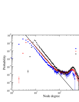
Figure 4: (Color online) Node-degree distributions for $\lambda=\pi$. The solid line gives a power law of exponent $-3.5$. Abscissae are log-binned.

For substantially smaller values of $\lambda$, notice first that, owing to the uniformity of the node distribution on the sphere, we expect $(1-\cos\rho^{t}_{i})n/2=n\sin^{2}(\rho^{t}_{i}/2)$ nodes to lie on node $i$’s spherical cap at time step $t$. This is then an upper bound on the expected value of $n^{t}_{i}$, node $i$’s degree in $G^{t}$. For fixed $\lambda$, it follows from the logarithmic dependency in Eq. (1) that this upper bound grows ever more slowly as $n^{t}_{i}$ increases. The latter, however, is ever less likely, since by Eq. (7) the process of increasing $n^{t}_{i}$ reflects back on itself negatively by increasing $c^{t}_{ij}$ regardless of $j$. It seems, then, that we are to expect node-degree distributions to undergo a somewhat sharp, $\lambda$-dependent cutoff at which probability may accumulate.

Node-degree distributions for values of $\lambda$ no greater than $0.5$ are given in Fig. 5. Notice that a power law does in fact get established that does not depend on $n$ or $\lambda$, but it is nevertheless subject to the cutoff mentioned above. The power-law regime lasts for increasingly larger stretches as $\lambda$ grows but ceases to hold as the cutoff is approached. For the larger values of $\lambda$ we do observe a certain accumulation of probability right before this point, but clearly nothing like the second power law of the $\lambda=\pi$ case seems to be happening now. If, as before, we now rescale the $\lambda$ parameter so that $\lambda\sqrt{n}$ remains constant as both $\lambda$ an $n$ vary, then by Fig. 6 we see that node degrees are limited by a cutoff value of about $80$. The plots in this figure are all such that $\lambda\sqrt{n}\approx 11$, which by Fig. 3 corresponds to the point beyond which the rescaling is no longer effective. Not only this, but from Fig. 3 we expect node-degree distributions to change significantly past this point, eventually approaching the distributions of Fig. 4 (the $\lambda=\pi$ case).

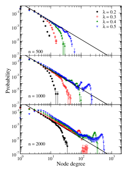
Figure 5: (Color online) Node-degree distributions for $\lambda\leq 0.5$. The solid lines give a power law of exponent $-2.6$. Abscissae are log-binned.

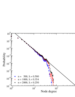
Figure 6: (Color online) Node-degree distributions for $\lambda\leq 0.5$ such that $\lambda\sqrt{n}$ is constant. The solid line gives a power law of exponent $-2.6$. Abscissae are log-binned.

One final set of plots is given in Fig. 7 for $\lambda\leq 0.5$ to illustrate the interdependency of distances on the graph and geodesic distances. Instead of plotting distances on the graph against geodesic distances directly, we first try to minimize the dependency on $n$ by once again evoking the uniform distribution of nodes on the sphere. Once we do this, it makes more sense to rescale each geodesic distance $\delta$ to the surface area of the spherical cap on which no two nodes are farther apart (geodesic-wise) than $2\delta$. If we further normalize to the surface area of the entire sphere, then the variable against which to plot distances on the graph is $(1-\cos\delta)/2=\sin^{2}(\delta/2)$. The resulting plots indicate an approximately linear growth of the distance on the graph, especially for the larger values of $\lambda$ or $\delta$. The rate of growth is less pronounced for larger values of $\lambda$ or $n$: in either case, distances on the graph are expected to be relatively insensitive to the geodesic distances.

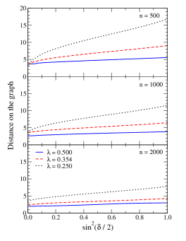
Figure 7: (Color online) Average distances on the graph as a function of geodesic distances for $\lambda\leq 0.5$. Abscissae correspond to $100$ fixed-width bins on the interval $[0,\pi]$.

In order to understand these trends, consider any two nodes $i$ and $j$ and recall that $\delta_{ij}$ is the geodesic distance between them. Depending on $\lambda$, the chance these two nodes constitute a feasible pair in terms of (4) varies considerably. When (4) does hold for some $t$, which by Eq. (1) tends to happen more often for the larger values of $\lambda$ or the larger values of $n$, establishing a direct connection between $i$ and $j$ once the two nodes have been selected depends exclusively on the gain-cost trade-off, which is a function of the current graph’s topology and independent of $\delta_{ij}$. When (4) does not hold, and this is more often observed for the smaller values of $\lambda$ or the smaller values of $n$, nodes $i$ and $j$ do not become directly interconnected just then and the distance between them on the graph tends to be larger for larger $\delta_{ij}$.

Figure 7 also helps complete our understanding of why the behavior of the mean node degree depends on $n$ for $\lambda\sqrt{n}>11$ in Fig. 3. Recall first that the motivation for the rescaling to $\lambda\sqrt{n}$ has been to keep the expected number of nodes on a node’s spherical cap fixed as both $\lambda$ and $n$ vary, and therefore induce an invariant expected behavior as far as the gain-cost trade-offs are concerned. What Fig. 7 indicates, however, is that distances on the graph depend on geodesic distances in different ways for fixed $\lambda\sqrt{n}$, and by Eq. (5) so do gains, since they depend crucially on distances on the graph. Our trade-offs can then be expected to operate differently for different values of $n$ even for fixed $\lambda\sqrt{n}$, indicating that in general it is not a spherical cap’s expected number of nodes that regulates their operation. But Fig. 7 also suggests that this effect is relatively negligible when $\sin^{2}(\delta/2)$ is very small. In fact, for all values of $\lambda\sqrt{n}$ up to about $11$, this is what happens in Fig. 3: in this range, we have mean node degrees of up to about $3$, and by Eq. (1) we expect to consider node pairs for joining that are no farther apart than some geodesic distance $\delta$ such that $\sin^{2}(\delta/2)<0.18$. This explains why the rescaling is effective in this region.

IV Conclusion

We have studied networks that grow from a fixed set of isolated nodes initially placed on the surface of a unit-radius sphere. Growth is promoted by considering node pairs that are not too far apart on the sphere and weighing, for each pair, a gain against a cost related to adding an edge between the two nodes. The edge is added to the network if the gain surpasses the cost. Our study has touched several relevant issues, such as the connectivity properties of the graph into which the network settles, the node-degree distribution of this graph, and also the relationship that exists between distances on the graph and geodesic distances.

Our mechanism of network growth depends crucially on the parameter, here called $\lambda$, that regulates, for each node and in a function of its current degree, the maximum geodesic distance to any node to which it may be connected by an edge in the graph. Relatively low values of $\lambda$ are attractive because they lend an additional degree of plausibility to the growth mechanism by letting nodes depend exclusively on locally available information to decide whether to get joined by an edge. We have found, by means of computer simulations, that node degrees at such values of $\lambda$ are distributed according to a fixed-exponent power law, provided $\lambda$ and $n$, the number of nodes, are such that $\lambda\sqrt{n}$ remains constant and bounded. For the cost parameters we used, the required bound on $\lambda\sqrt{n}$ is about $11$, and the power-law exponent is $-2.6$. This rescaling of $\lambda$ to $\lambda\sqrt{n}$ is based on the assumption that nodes are distributed uniformly over the sphere, and we have found it to provide a certain degree of independence of $n$ in questions related to network connectivity as well.

This paper’s study generalizes and extends our own previous work of Barbosa et al. (2006), respectively by using geometric coordinates to limit the reach of new edges as they enter the network, and by addressing issues other than that of node-degree distributions. What the two works have in common is the use of closely related gain-cost trade-offs as the main drives of network growth. The fact that, in essence, scale-free properties appear in both models seems to confirm that trade-offs such as the ones we have used have an important role to play in the evolution of real-world computer networks.