Thermodynamics and superfluid density in BCS-BEC crossover with and without population imbalance

Abstract

We address the thermodynamics, density profiles and superfluid density of trapped fermions undergoing BCS-BEC crossover. We consider the case of zero and finite population imbalance. Our approach represents a fully consistent treatment of ”pseudogap effects”. These effects reflect the distinction between the pair formation temperature $T^{*}$ and the pair condensation temperature $T_{c}$. As a natural corollary, this temperature difference must be accommodated by modifying the fermionic excitation spectrum $E_{\mathbf{k}}$ to reflect the fact that fermions are paired at and above $T_{c}$. It is precisely this natural corollary which has been omitted from all other many body approaches in the literature. At a formal level, we show how enforcing this corollary implies that pairing fluctuation or self energy contributions enter into both the gap and the number equations; this is necessary in order to be consistent with a generalized Ward identity. At a less formal level, we demonstrate that we obtain physical results for the superfluid density $n_{s}(T)$ at all temperatures. In contrast, previous work in the literature has led to non-monotonic, or multi-valued or discontinuous behavior for $n_{s}(T)$. Because it reflects the essence of the superfluid state, we view the superfluid density as a critical measure of the physicality of a given crossover theory. In a similarly unique fashion, we emphasize that in order to properly address thermodynamic properties of a trapped Fermi gas, a necessary first step is to demonstrate that the particle density profiles are consistent with experiment. Without a careful incorporation of the distinction between the pairing gap and the order parameter, the density profiles tend to exhibit sharp features at the condensate edge, which are never seen experimentally in the crossover regime. The lack of demonstrable consistency between theoretical and experimental density profiles, along with problematic behavior found for the superfluid density, casts doubt on previous claims in the literature concerning quantitative agreement between thermodynamical calculations and experiment.

I Introduction

There has been a resurgence of interest in studies of the crossover between the usual BCS form of fermionic superfluidity and that associated with Bose Einstein condensation (BEC). This is due, in part, to the widespread pseudogap phenomena which have been observed in high temperature superconductors in conjunction with the small pair size. The latter, in particular, was argued by Leggett to be a rationale Leggett (2006) for treating the cuprates as mid-way between BCS and BEC. Others have argued Randeria (1995); Chen et al. (2005a); Levin and Chen that the cuprate pseudogap can be understood as arising from pre-formed pairs which form due to the stronger-than-BCS attraction. Additional reasons for the interest in BCS-BEC crossover stem from the precise realization of this scenario in ultracold trapped Fermi gases,Chen et al. (2005a) where the attractive interaction can be continuously tuned from weak to strong via a Feshbach resonance in the presence of a magnetic field. A final rationale for interest in this problem stems from the fact that BCS theory is the prototype for successful theories in condensed matter physics; and we now have come to realize that this is a very special case of a much more general class of superfluidity.

BCS-BEC crossover theory is based on the observation Eagles (1969); Leggett (1980) that the usual BCS ground state wave function $\Psi_{0}=\Pi_{\bf k}(u_{\mathbf{k}}+v_{\mathbf{k}}c_{\bf k,\uparrow}^{\dagger}c_{\bf-k,\downarrow}^{\dagger})|0\rangle$ (where $c^{\dagger}_{\bf k,\sigma}$ and $c_{\bf k,\sigma}$ are the creation and annihilation operators for fermions of momentum ${\bf k}$ and spin $\sigma=\uparrow,\downarrow$) is far more general than was initially appreciated. If one tunes the attractive interaction from weak to strong, along with a self consistent determination of the variational parameters $v_{\mathbf{k}}$ and $u_{\bf k}$ the chemical potential passes from positive to negative and the system crosses continuously from BCS to BEC. The vast majority (with the possible exception of the high $T_{c}$ cuprates) of metallic superconductors are associated with weak attraction and large pair size. Thus, this more generalized form of BCS theory was never fully characterized or exploited until recently. There are a number of different renditions of BCS-BEC crossover theory. Each rendition can be represented by a selected class of many-body Feynman diagrams, often further simplified by various essential or non-essential approximations. There is no controlled small parameter and thus the selection process is based on highly variable criteria. For the most part the success or failure of a particular rendition is evaluated by comparing one or a set of numbers with experiment.

It is the goal of the present paper to discuss a criteria set for evaluating BCS-BEC crossover theories which captures the crucial physics, rather than the detailed numerics. We apply these criteria successfully to one particular version of BCS-BEC crossover theory which builds on the above ground state. In this context we address a wide range of physical phenomena. These include density profiles, thermodynamical properties and superfluid density with application to polarized as well as unpolarized gases. It is our philosophy that appropriate tests of the theory should relate to how qualitatively sound it is before assessing it in quantitative detail. Detailed quantitative tests are essential but if the qualitative physics is not satisfactory, quantitative comparisons cannot be meaningful.

Four important and inter-related physical properties are emphasized here. (i) There must be a consistent treatment of “pseudogap” effects.Levin and Chen As a consequence of the fact that the pairing onset temperature $T^{*}$ is different Micnas et al. (1990); Randeria (1995) from the condensation temperature $T_{c}$, the fermionic spectrum, $E_{\mathbf{k}}$ must necessarily reflect the formation of these pairs. To accommodate the pseudogap, $E_{\mathbf{k}}$ must be modified from the strict BCS form which has a vanishing excitation gap at and above $T_{c}$. Everywhere in the literature an unphysical form for $E_{\mathbf{k}}$ is assumed except in our own work and briefly in Ref. Pieri and Strinati, 2005. (ii) The theory must yield a consistent description of the superfluid density $n_{s}(T)$ from zero to $T_{c}$. The quantity $n_{s}(T)$ should be single valued, monotonic, NsF and disappear at the same $T_{c}$ one computes from the normal state instability. Importantly, $n_{s}(T)$ is at the heart of a proper description of the superfluid phase. (iii) The behavior of the density profiles, which are the basis for computing thermodynamical properties of trapped gases, must be compatible with experimental measurements. Near and at unitarity, and in the absence of population imbalance, they are relatively smooth and featureless, unlike a true BEC where there is clear bimodality. This can present a challenge for theories which do not accommodate pseudogap effects and which then deduce sharp features at the condensate edge. (iv) The thermodynamical potential $\Omega$ should be variationally consistent with the gap and number equations. It should satisfy appropriate Maxwell relations and at unitarity be compatible with the constraint Ho (2004); Thomas et al. (2005) relating the pressure $p$ to the energy, $E$: $p=\frac{2}{3}E$.

There has been widespread discussion about the role of collective modes in the thermodynamics of fermionic superfluids. And this has become, in some instances, a basis for additional evaluation criteria of a given BCS-BEC crossover theory. Because the Fermi gases represent neutral superfluids with low lying collective modes, one might have expected these modes to be more important than in charged superconductors. Nevertheless, the BCS wave function and its associated finite temperature behavior is well known to work equally well for charged superconductors and neutral superfluids such as helium-3. In strict BCS theory thermodynamical properties are governed only by fermionic excitations. This applies as well to the superfluid density (in the transverse gauge). Collective modes are important in strict BCS theory primarily to establish that $n_{s}(T)$ is properly gauge invariant.

One can argue Nozières and Schmitt-Rink (1985) that collective modes should enter thermodynamics as the pairing attraction becomes progressively stronger. The role of these modes at unitarity is currently unresolved. In the Bogoliubov description of a true Bose superfluid there is a coupling between the pair excitations and the collective modes, which results from inter-boson interactions. Thus it is reasonable to expect that the collective modes are important for thermodynamical properties in the BEC regime. At the level of the simple mean BCS-Leggett wave function we find that, just as in strict BCS theory, the collective modes do not couple to the pair excitations; this leads to a $q^{2}/2M^{*}$ form of the pair dispersion. The low-lying collective mode dispersion is,Kosztin et al. (2000) of course, linear in $q$. All inter-boson effects are treated in a mean field sense and enter to renormalize the effective pair mass $M^{*}$. To arrive at a theory more closely analogous to Bogoliubov theory, one needs to add additional terms to the ground state wave function– consisting of four and six creation operators Tan and Levin (2006) in the deep BEC. The complexity becomes even greater in the unitary regime, and there is, in our opinion, no clear indication one way or the other on how the pair excitations and collective modes couple.

Our rationale for considering the simplest ground state wave function (which minimizes this coupling) is as follows. It is the basis for zero temperature Bogoliubov-de Gennes (BdG) approaches which have been widely applied to the crossover problem. It is the basis for a $T=0$ Gross-Pitaevskii description in the far BEC regime.Pieri and Strinati (2003) It is the basis for the bulk of the work on population imbalanced gases. At unitarity the universality relation Ho (2004); Thomas et al. (2005) between pressure and energy holds – separately for the fermionic contribution (which is of the usual BCS form with an excitation gap distinct from the order parameter) and for the bosonic term, due to the $q^{2}$ form of the pair dispersion. Finally, this wave function is simple and accessible. Thus, it seems reasonable to begin by addressing the finite $T$ physics which is associated with this ground state, in a systematic way.

The remainder of this paper presents first the theoretical framework for the principal self consistent equations describing the total excitation gap, the order parameter, and the number equation or fermionic chemical potential. The consequences for thermodynamics, density profiles and the superfluid density are then presented in separate sections, along with numerically obtained results for each property. We discuss these properties at the qualitative as well as semi-quantitative level, in the context of comparison with experiment. In the conclusions section, we present a summary of the strengths and weaknesses of the present scheme.

II Theoretical Background

II.1 Early Relevant History of BCS-BEC Crossover

While the subject began with the seminal $T=0$ work by Eagles Eagles (1969) and Leggett,Leggett (1980) a discussion of superfluidity beyond the ground state was first introduced into the literature by Nozieres and Schmitt-Rink. Nozières and Schmitt-Rink (1985) Randeria and co-workers reformulated this approach Nozières and Schmitt-Rink (1985) and moreover, raised the interesting possibility that crossover physics might be relevant to high temperature superconductors Randeria (1995). Subsequently other workers have applied this picture to the high $T_{c}$ cuprates Chen et al. (1998); Micnas and Robaszkiewicz (1998); Ranninger and Robin (1996); Perali et al. (2002) and ultracold Fermi gases Milstein et al. (2002); Ohashi and Griffin (2002) as well as formulated alternative schemes Ohashi and Griffin (2003); Pieri et al. (2004) for addressing $T\neq 0$.

The recognition that one should distinguish the pair formation temperature $T^{*}$ from the condensation temperature $T_{c}$ was crucial. Micnas et al. (1990); Randeria (1995) Credit goes to those who noted that pseudogap effects would appear in the BCS-BEC crossover scenario of high temperature superconductors, notably first in the spin channel. Trivedi and Randeria (1995) Shortly thereafter, it was recognized that these important pseudogap phenomena also pertain to the charge channel. Jankó et al. (1997); Chen et al. (1999, 1998) And finally, we make note of those papers where the concept of pseudogap effects was introduced into studies of the ultra-cold gases. Stajic et al. (2004); Pieri et al. (2004); Chen et al. (2005a)

II.2 Pair Fluctuation Approaches to Crossover

In this section we discuss the present scheme for BCS-BEC crossover, as well as compare it with alternative approaches including that of Nozieres and Schmitt-Rink. Nozières and Schmitt-Rink (1985) The Hamiltonian for BCS-BEC crossover can be described by a one-channel model. In this paper, we address primarily a short range $s$-wave pairing interaction, which is often simplified as a contact potential $U\delta(\mathbf{x-x^{\prime}})$, where $U<0$. This Hamiltonian has been known to provide a good description for the crossover in atomic Fermi gases which have very wide Feshbach resonances, such as ⁴⁰K and ⁶Li. The details are presented elsewhere. Chen et al. (2005a)

We begin with a discussion of T-matrix based theories. Within a T-matrix scheme one considers the coupled equations between the particles (with propagator $G$) and the pairs [which can be represented by the $T$-matrix $t(Q)$] and drops all higher order terms. Without taking higher order Green’s functions into account, the pairs interact indirectly via the fermions, in an averaged or mean field sense. The propagator for the non-condensed pairs is given by

$$t_{pg}^{-1}(Q)=U^{-1}+\chi(Q)\,,$$ (1)

where $U$ is the attractive coupling constant in the Hamiltonian and $\chi$ is the pair susceptibility. The function $\chi(Q)$ is the most fundamental quantity in T-matrix approaches. It is given by the product of dressed and bare Green’s functions in various combinations. One could, in principle, have considered two bare Green’s functions or two fully dressed Green’s functions. Here, we follow the work of Ref.  Kadanoff and Martin, 1961. These authors systematically studied the equations of motion for the Green’s functions associated with the usual many body Hamiltonian for superfluidity and deduced that the only satisfactory truncation procedure for these equations involves a T-matrix with one dressed and one bare Green’s function. The presence of the bare Green’s function in the $T$-matrix and self-energy is a general, inevitable consequence of an equations of motion procedure. Chen (2000)

In this approach, the pair susceptibility is then

$$\hskip 28.45274pt\chi(Q)=\sum_{K}G_{0}(Q-K)G(K),\qquad$$ (2)

where $Q=(i\Omega_{l},\mathbf{q})$, and $G$ and $G_{0}$ are the full and bare Green’s functions respectively. Here $G_{0}^{-1}(K)=i\omega_{n}-\xi_{\mathbf{k}}$, $\xi_{\mathbf{k}}=\epsilon_{\mathbf{k}}-\mu$, $\epsilon_{\mathbf{k}}=\hbar^{2}k^{2}/2m$ is the kinetic energy of fermions, and $\mu$ is the fermionic chemical potential. Throughout this paper, we take $\hbar=1$, $k_{B}=1$, and use the four-vector notation $K\equiv(i\omega_{n},\mathbf{k})$, $Q\equiv(i\Omega_{l},\mathbf{q})$, $\sum_{K}\equiv T\sum_{n}\sum_{\bf k}$, etc, where $\omega_{n}=(2n+1)\pi T$ and $\Omega_{l}=2l\pi T$ are the standard odd and even Matsubara frequencies Fetter and Walecka (1971) (where $n$ and $l$ are integers).

The one-particle Green’s function is

$$G^{-1}(K) = i\omega_{n}-\xi_{k}-\Sigma(K)\,,$$ (3)

where

$$\hskip 28.45274pt\Sigma(K)=\sum_{Q}t(Q)G_{0}(Q-K),\qquad$$ (4)

More generally, either $G_{0}$ or the fully dressed $G$ is introduced into $\Sigma(K)$, according to the chosen $T$-matrix scheme. Finally, in terms of Green’s functions, we readily arrive at the number equation: $n=\sum_{K,\sigma}G_{\sigma}(K)$.

Because of interest from high temperature superconductivity, alternate schemes, which involve only dressed Green’s functions have been rather widely studied. In one alternative, one constructs a thermodynamical potential based on a chosen self-energy. Here there is some similarity to that $T$-matrix scheme which involves $G$ only. One variant of this “conserving approximation” is known as the fluctuation exchange approximation (FLEX) which has been primarily applied to the normal state. In addition to the particle-particle ladder diagrams which are crucial to superfluidity it also includes less critical diagrams in the particle-hole channel; the latter can be viewed as introducing spin correlation effects. Since it involves only dressed Green’s functions, one evident advantage of this approach is that it is $\Phi$-derivable Baym (1962) or conserving. This implies that because it is based on an analytical expression for the thermodynamical potential, thermodynamical quantities obtained by derivatives of the free energy are identical to those computed directly from the single particle Green’s function.

For a variety of reasons this FLEX scheme, as applied to superfluids and superconductors, has been found to be problematic. The earliest critique of the $GG$, T-matrix scheme is in Ref. Kadanoff and Martin, 1961. The authors noted that using two dressed Green’s functions “could be rejected by means of a variational principle”. They also observed that there would be an unphysical consequence: a low $T$ specific heat which contained a contribution proportional to $T^{2}$. In a related fashion it appears that the FLEX or $GG$, T-matrix scheme is not demonstrably consistent with the Hamiltonian-based equations of motion. There also is concern that considering only dressed fermion propagators, $G$, may lead to double counting of Feynman diagrams. Vilk et al Vilk and Tremblay (1997) noted that the FLEX scheme will not produce a proper pseudogap, due to the “inconsistent treatment of vertex corrections in the expression for the self energy.”

By dropping the non-dominant particle-hole diagrams, others have found a more analytically tractable scheme Tchernyshyov (1997). However, this scheme fails to yield back BCS-like spectral properties which would be anticipated above $T_{c}$ in a BCS-BEC crossover scenario. Among the unusual features found is a four excitation branch structure, Singer et al. (1997); Pedersen et al. (1997) not compatible with the expected pseudogap description, which should reflect precursor superconductivity effects in the normal state. In this pseudogap picture, Chen et al. (2005a) there would be two peaks in the spectral function, rather than four. More recently, the authors of Ref. Haussmann et al., 2007 applied a related conserving approximation below $T_{c}$. They did not consider particle-hole diagrams, but included in the particle-particle channel a “twisted” ladder diagram. These authors found that there was a discontinuity in the transition temperature calculated relative to that computed Haussmann (1993) above $T_{c}$. They, then, inferred that at unitarity there is a first order phase transition, which has not been experimentally observed.

In the NSR scheme, which is, perhaps, the most widely applied of all pair fluctuation theories, one uses two bare Green’s functions in $\chi(Q)$ for the normal state. Within this NSR approach, the results are generally extended below $T_{c}$ by introducing Perali et al. (2004a) into $\chi(Q)$ the diagonal and off-diagonal forms of the Nambu-Gor’kov Greens functions. At the outset, the fermionic excitation spectrum $E_{\mathbf{k}}=\sqrt{\xi_{\mathbf{k}}^{2}+\Delta_{sc}^{2}}$ involves only the superfluid order parameter, $\Delta_{sc}$, so that the fermions are treated as gapless at and above $T_{c}$, despite the fact that there is an expected “pseudogap” associated with pairing onset temperature $T^{*}$. The original authors Nozières and Schmitt-Rink (1985) suggested that pair fluctuations should enter into the number equation, but approximated their form based on only the leading contribution in the Dyson series. This approximate form was introduced via contribution to the thermodynamical potential $\Omega$. A more systematic approach, which is based on a full Dyson resummation leads to a form equivalent to Eq. (4), with a bare $\chi_{0}(Q)=\sum_{K}G_{0}(K)G_{0}(Q-K)$, as was first pointed out in Ref. Serene, 1989. This more complete scheme was implemented in Ref. Perali et al., 2004a.

Another important aspect of the NSR scheme should be noted. Because the pairing fluctuation contributions do not enter into the gap equation, the gap equation cannot be determined from a variational condition on the thermodynamic potential. In this regard, a rather different alternative to the approximated number equation of Ref. Nozières and Schmitt-Rink, 1985 was recently introduced in Ref. Dru, a, b. These authors argued one should compensate for the fact that $d\Omega/d\Delta_{sc}\neq 0$ by adding a new term (deriving from this discrepancy) to the number equation. We view this latter alternative as even more problematic since it builds on inconsistencies within the NSR approach in both the gap and the number equation. By far the most complete study of the NSR based theory for crossover was summarized in Ref. Pieri and Strinati, 2005. By systematically introducing a series of improved approximations, the authors ultimately noted that one must incorporate pairing fluctuation corrections into the gap as well as the number equation.

It should be stressed that (with or without the approximate form for the number equation) the NSR scheme at $T\neq 0$ was not designed to be consistent with the simple BCS-Leggett ground state, which they also discussed at length. This observation was implicitly made elsewhere Perali et al. (2004b) in the literature and can be verified by comparing the ground state density profiles based on the NSR scheme with those obtained in the Leggett mean field theory. Perali et al. (2004b) It should also be stressed that T-matrix theories do not incorporate a direct pair-pair interaction; rather the pairs interact in an average or mean field sense. If one tries to extract the effective pairing interaction from any $T$-matrix theory, the absence of coupling to higher order Green’s functions will lead to a simple factor of two relating the inter-boson and inter-fermion scattering lengths. More exact calculations of this ratio lead to a factor of 0.6. Petrov et al. (2004); Tan and Levin (2006); Pieri and Strinati (2006); Brodsky et al. (2006)

II.3 Present T-matrix Scheme

We now show that one obtains consistent answers between $T$-matrix based approaches and the BCS-Leggett ground state equations, provided the pair susceptibility contains one bare and one dressed Green’s function. Thus, for simplicity, we refer to the present approach as “$GG_{0}$ theory”. Throughout this paper we will emphasize the strengths of the present T-matrix scheme which rest primarily on a consistent treatment of pseudogap effects in the gap and number equations. This, in turn, leads to physical behavior for the thermodynamics, the superfluid density and the density profiles at all temperatures. Finally, we note that the present T-matrix scheme is readily related to a previously studied Patton (1971) approach to fluctuations in low dimensional, but conventional superconductors. A weak coupling limit of this $GG_{0}$ approach is equivalent to Hartree approximated Ginzburg-Landau theory. Stajic et al. (2004)

We begin with the situation in which there is an equal spin mixture, and then generalize to the population imbalanced case. In the present formalism, for all $T\leq T_{c}$, the gap equation is associated with a BEC condition which requires that the pair chemical potential $\mu_{pair}$ vanish. We will show below that because of this vanishing of $\mu_{pair}$ at and below $T_{c}$, to a good approximation one can move $G_{0}$ outside the summation in Eq. (4). As a result the self-energy is of the BCS-like form

$$\Sigma(K)=-\Delta^{2}G_{0}(-K)=\frac{\Delta^{2}}{i\omega_{n}+\xi_{k}}\,.$$ (5)

Thus

$$G^{-1}(K)=i\omega_{n}-\xi_{k}-\frac{\Delta^{2}}{i\omega_{n}+\xi_{k}}\,.$$ (6)

Now we are in a position to calculate the pair susceptibility at general $Q$, based on Eq. (2). After performing the Matsubara sum and analytically continuing to the real axis, $i\Omega_{l}\rightarrow\Omega+i0$) we find the relatively simple form

$$\chi(Q) = \sum_{\bf k}\Big{[}\frac{1-f(E_{\bf k})-f(\xi_{\bf k-q})}{E_{\bf k}+\xi_{\bf k-q}-\Omega-i0^{+}}u_{\bf k}^{2}$$ (7)

$${}-\frac{f(E_{\bf k})-f(\xi_{\bf k-q})}{E_{\bf k}-\xi_{\bf k-q}+\Omega+i0^{+}}v_{\bf k}^{2}\Big{]}\,,$$

where $u_{\mathbf{k}}^{2},v_{\mathbf{k}}^{2}=(1\pm\xi_{\mathbf{k}}/E_{\mathbf{k}})/2$ are the usual coherence factors, and $f(x)$ is the Fermi distribution function. It follows that $\chi(0)$ is given by

$$\chi(0)=\sum_{\mathbf{k}}\frac{1-2{f}(E_{k})}{2E_{k}}$$ (8)

The vanishing of $\mu_{pair}$ (or generalized Thouless criterion) then implies that

$$t_{pg}^{-1}(0)=U^{-1}+\chi(0)=0,\qquad T\leq T_{c}\;.$$ (9)

Substituting $\chi(0)$ into the above BEC condition, we obtain the familiar gap equation

$$0 = \frac{1}{U}+\sum_{\mathbf{k}}\frac{1-2{f}(E_{k})}{2E_{k}}\,.$$ (10)

Here $E_{\mathbf{k}}=\sqrt{\xi_{\mathbf{k}}^{2}+\Delta^{2}}$, which contains the total excitation gap $\Delta$ instead of the order parameter $\Delta_{sc}$.

The coupling constant $U$ can be replaced in favor of the dimensionless parameter, $1/k_{F}a$, via the relationship $m/(4\pi a)=1/U+\sum_{\mathbf{k}}(2\epsilon_{k})^{-1}$, where $a$ is the two-body $s$-wave scattering length, and $k_{F}$ is the noninteracting Fermi wave vector for the same total number density. Therefore the gap equation can be rewritten as

$$-\frac{m}{4\pi a}=\sum_{\mathbf{k}}\left[\frac{1-2{f}(E_{k})}{2E_{k}}-\frac{1}{2\epsilon_{k}}\right]\,.$$ (11)

Here the “unitary scattering” limit corresponds to resonant scattering where $a\rightarrow\infty$. For atomic Fermi gases, this scattering length is tunable via a Feshbach resonance by application of a magnetic field and we say that we are on the BCS or BEC side of resonance, depending on whether the fields are higher or lower than the resonant field, or alternatively whether $a$ is negative or positive, respectively.

Finally, inserting the self energy of Eq. (5), into the Green’s function, it follows that the number equation is given by

$$n = 2\sum_{\mathbf{k}}[f(E_{k})u_{\mathbf{k}}^{2}+f(-E_{k})v_{\mathbf{k}}^{2}]\,,$$ (12)

thus demonstrating that both the number and gap equation [see Eq. (10)] are consistent with the ground state constraints in BCS-Leggett theory.

Next we use this $T$-matrix scheme to derive Eq. (5) and separate the contribution from condensed and noncondensed pairs. The diagrammatic representation of our $T$-matrix scheme is shown in Fig. 1. The first line indicates the $T$-matrix, $t_{pg}$, and the second the total self energy. The $T$-matrix can be effectively regarded as the propagator for noncondensed pairs. One can see throughout the combination of one dressed and one bare Green’s function, as represented by the thick and thin lines. The self energy consists of two contributions from the noncondensed pairs or pseudogap ($pg$) and from the condensate ($sc$). There are, analogously, two contributions to the full $T$-matrix

$$t = t_{pg}+t_{sc}\,,$$ (13)

$$t_{pg}(Q) = \frac{U}{1+U\chi(Q)},\qquad Q\neq 0\,,$$ (14)

$$t_{sc}(Q) = -\frac{\Delta_{sc}^{2}}{T}\delta(Q)\,,$$ (15)

where we write $\Delta_{sc}=-U\sum_{\bf k}\langle c_{-{\bf k}\downarrow}c_{{\bf k}\uparrow}\rangle$. Similarly, we have for the fermion self energy

$$\Sigma(K)=\Sigma_{sc}(K)+\Sigma_{pg}(K)=\sum_{Q}t(Q)G_{0}(Q-K)\,.$$ (16)

We see at once that

$$\Sigma_{sc}(K)=\sum_{Q}t_{sc}(Q)G_{0}(Q-K)=-G_{0}(-K)\Delta_{sc}^{2}\,.$$ (17)

A vanishing chemical potential means that $t_{pg}(Q)$ diverges at $Q=0$ when $T\leq T_{c}$. Thus, we approximate Maly et al. (1999a) Eq. (16) to yield

$$\Sigma(K)\approx-G_{0}(-K)\Delta^{2}\,,$$ (18)

where

$$\Delta^{2}(T)\equiv\Delta_{sc}^{2}(T)+\Delta_{pg}^{2}(T)\,,$$ (19)

Importantly, we are led to identify the quantity $\Delta_{pg}$

$$\Delta_{pg}^{2}\equiv-\sum_{Q\neq 0}t_{pg}(Q).$$ (20)

Note that in the normal state (where $\mu_{pair}$ is non-zero), Eq. (18) is no longer a good approximation. We now have a closed set of equations for addressing the ordered phase. We show later how to extend this approach to temperatures somewhat above $T_{c}$, by self consistently including a non-zero pair chemical potential. This is a necessary step in addressing a trap as well. Chien et al. (2006a)

The propagator for noncondensed pairs can now be quantified, using the self consistently determined pair susceptibility. At small four-vector $Q$, we may expand the inverse of $t_{pg}$, after analytical continuation, to obtain

$$t_{pg}^{-1}(Q)\approx a_{1}\Omega^{2}+Z\left(\Omega-\frac{q^{2}}{2M^{*}}+\mu_{pair}+i\Gamma_{Q}\right),$$ (21)

where below $T_{c}$ the imaginary part $\Gamma_{Q}\rightarrow 0$ faster than $q^{2}$ as $q\rightarrow 0$. Because we are interested in the moderate and strong coupling cases, where the contribution of the $a_{1}\Omega^{2}$ term is small, we drop it in Eq. (21) so that

$$t_{pg}(Q)=\frac{Z^{-1}}{\Omega-\Omega_{q}+\mu_{pair}+i\Gamma_{Q}},$$ (22)

where we associate

$$\Omega_{\mathbf{q}}\approx\frac{q^{2}}{2M^{*}}\,.$$ (23)

This establishes a quadratic pair dispersion and defines the effective pair mass, $M^{*}$. This can be calculated via a small $q$ expansion of $\chi(Q)$,

$$Z=\left.\frac{\partial\chi}{\partial\Omega}\right|_{\Omega=0,\mathbf{q}=0},\qquad\frac{1}{2M^{*}}=-\left.\frac{1}{6Z}\frac{\partial^{2}\chi}{\partial q^{2}}\right|_{\Omega=0,\mathbf{q}=0}\,.$$ (24)

Finally, one can rewrite Eq. (20) as

$$\Delta_{pg}^{2}(T)=Z^{-1}\sum_{\mathbf{q}}b(\Omega_{q}),$$ (25)

where $b(x)$ is the Bose distribution function.

Figure 1: $T$-matrix and self-energy diagrams for the present $T$-matrix scheme. The self-energy comes from contributions of both condensed ($\Sigma_{sc}$) and noncondensed ($\Sigma_{pg}$) pairs. Note that there is one dressed and full Green’s function in the $T$-matrix. Here the $T$-matrix $t_{pg}$ can be regarded effectively as the propagator for the noncondensed pairs.

The superfluid transition temperature $T_{c}$ is determined as the lowest temperature(s) in the normal state at which noncondensed pairs exhaust the total weight of $\Delta^{2}$ so that $\Delta_{pg}^{2}=\Delta^{2}$. Solving for the “transition temperature” in the absence of pseudogap effects Machida et al. (2006); Yi and Duan (2006); Ric leads to the quantity $T_{c}^{MF}$. More precisely, $T_{c}^{MF}$ should be thought of as the temperature at which the excitation gap $\Delta(T)$ vanishes. This provides a reasonable estimate for the pairing onset temperature $T^{*}$. It is to be distinguished from $T_{c}$, below which a stable superfluid phase exists. We note that $T^{*}$ represents a smooth crossover rather than a thermodynamic phase transition.

It should be stressed that the dispersion relation for the noncondensed pairs is quadratic. While one will always find a linear dispersion in the collective mode spectrum, Kosztin et al. (2000) within the present class of BCS-BEC crossover theories, the restriction to a $T$-matrix scheme means that there is no feedback from the collective modes onto the pair excitation spectrum. In effect, the $T$-matrix approximation does not incorporate pair-pair interactions at a level needed to arrive at this expected linear dispersion in the pair excitation spectrum. Nevertheless, this level of approximation is consistent with the underlying ground state wave function.

III Generalization to Include Population Imbalance

It is relatively straightforward to include a difference in particle number between the two spin species, within the context of the BCS-Leggett wave function. This is closely analogous to solving for the spin susceptibility in BCS theory. The excitation energies are given by $E_{k\uparrow}=-h+E_{k}$ and $E_{k\downarrow}=h+E_{k}$, where $\xi_{k}=\epsilon_{k}-\mu$ and $E_{\mathbf{k}}=\sqrt{\xi_{\mathbf{k}}^{2}+\Delta^{2}}$. Here $\mu=(\mu_{\uparrow}+\mu_{\downarrow})/2$ and $h=(\mu_{\uparrow}-\mu_{\downarrow})/2$. We assume spin up fermions are the majority so that $n_{\uparrow}>n_{\downarrow}$ and $h>0$. It is important to note that depending on $h$, $\mu$, and $\Delta$, the quantity $E_{k\uparrow}$ may on occasion assume negative values for a bounded range of $k$-states. At $T=0$ this implies that there are regimes in $k$-space in which no minority component is present. This leads to what is often referred to as a “gapless” phase. It was first studied by Sarma Sarma (1963) at $T=0$ in the BCS regime.

It is natural to extend this ground state Sarma or “breached pair” phase to include BCS-BEC crossover effects Pao et al. (2006); Sheehy and Radzihovsky (2006); De Silva and Mueller (2006); Haque and Stoof (2006). The effects of finite temperatures were also studied using the current $GG_{0}$, T-matrix scheme Yi and Duan (2006); Chien et al. (2006a, b); Chen et al. (2006a), using the Nozieres Schmitt-Rink formalism Parish et al. (2007) as well as using an alternative many body approach. Haque and Stoof (2006); Ric It should be noted, however, that the Sarma phase is generally not stable at $T=0$ except on the BEC side of resonance. Studies of the Sarma phase closer to unitarity and at low temperature reveal negative superfluid density Pao et al. (2006) as well as other indications for instability. Chen et al. (2006a) More generally, closer to unitarity, the Sarma phase stabilizes only at intermediate temperatures, Chien et al. (2006b) while the ground state appears to exhibit phase separation.

The notion of phase separation between paired and unpaired states, separated by an interface, was first introduced in Cal in the BCS limit, and it was more extensively discussed at $T=0$ in the crossover regime in Ref. Sheehy and Radzihovsky, 2006 for the homogeneous case. A treatment of phase separation in a trap at zero De Silva and Mueller (2006); Haque and Stoof (2006) and at finite temperature Chien et al., 2007; Ric, has received considerable recent attention. In a harmonic trap, phase separation leads to a nearly unpolarized gas at the center surrounded by a polarized, but essentially uncorrelated normal Fermi gas. Here one sees that the excitation gap $\Delta$ decreases abruptly to zero. By contrast, at higher temperatures, where the Sarma phase is stabilized, $\Delta$ decreases to zero continuously and there is a highly correlated mixed normal region separating a superfluid core and normal (uncorrelated) gas.

We now extend the present $GG_{0}$ formalism to include polarization effects. Chen et al. (2007) Including explicit spin indices, the pair susceptibility is given by

$$\chi(Q)=\frac{1}{2}\big{[}\chi_{\uparrow\downarrow}(Q)+\chi_{\downarrow\uparrow}(Q)\big{]}$$

$$=\sum_{\mathbf{k}}\left[\frac{1-\bar{f}(E_{k})-\bar{f}(\xi_{q-k})}{E_{k}+\xi_{q-k}-i\Omega_{l}}u_{k}^{2}-\frac{\bar{f}(E_{k})-\bar{f}(\xi_{q-k})}{i\Omega_{l}+E_{k}-\xi_{q-k}}v_{k}^{2}\right],$$

where the coherence factors $u_{\mathbf{k}}^{2},v_{\mathbf{k}}^{2}=(1\pm\xi_{\mathbf{k}}/E_{\mathbf{k}})/2$ are formally the same as for an equal spin mixture. For notational convenience we define

$$\bar{f}(x)\equiv[f(x+h)+f(x-h)]/2,$$ (27)

Following the same analysis as for the unpolarized case, and using the above form for the pair susceptibility, the gap equation can be rewritten as

$$-\frac{m}{4\pi a}=\sum_{\mathbf{k}}\left[\frac{1-2\bar{f}(E_{k})}{2E_{k}}-\frac{1}{2\epsilon_{k}}\right]\,.$$ (28)

The mean field number equations can be readily deduced

$$n_{\sigma} = \sum_{\mathbf{k}}[f(E_{k\sigma})u_{\mathbf{k}}^{2}+f(-E_{k\bar{\sigma}})v_{\mathbf{k}}^{2}]\,,$$ (29)

where $\bar{\sigma}=-\sigma$. The pseudogap equation is then

$$\Delta_{pg}^{2}(T)=Z^{-1}\sum_{\mathbf{q}}b(\Omega_{q}).$$ (30)

Analytical expressions for $Z$ and $\Omega_{q}$ can be obtained via expansion of $\chi(Q)$ at small $Q$ (See, e.g., Ref. Chen et al., 2007). This theory can readily be extended to include a (harmonic) trap as will be discussed in more detail in Sec. VI. In case of a phase separation, equilibrium requires $T$, $\mu$, and and the pressure, $p$ to be continuous across the interface or domain wall. Finally, it is useful to define polarization $\delta$ in terms of

$$N_{\sigma}(r) = \int d^{3}r\,n_{\sigma}(r),\quad N=N_{\uparrow}+N_{\downarrow},$$ (31)

$$\delta = (N_{\uparrow}-N_{\downarrow})/N.$$ (32)

In this paper we do not discuss alternative phases such as the famous Larkin-Ovchinnikov-Fulde-Ferrell (LOFF) states FFL in which the condensate is associated with one or more non-zero momenta $\mathbf{q}$. The competition between various polarized phases is associated Chen et al. (2007) with the detailed structure of $\chi(Q)$. Indeed, there are strong similarities between these competing phases in polarized gases and Hartree-Fock theories which are used to establish whether ferro- or antiferromagnetic order will arise in a many body system. The latter is associated with zero or finite wave-vector, respectively, and depends on the nature of the particle-hole spin susceptibility, $\bar{\chi}^{part-hole}(Q)$. This, in turn, is given by $\bar{\chi}^{part-hole}(Q)\propto\bar{U}^{-1}+\bar{\chi}_{o}(Q)$, where $\bar{\chi}_{o}$ is the usual Lindhard function and $\bar{U}$ is the on-site repulsion. Here, by analogy the “ferromagnetic” case would correspond to the Sarma phase and the “antiferromagnetic” situation to a LOFF like phase. Note, however that the relevant $\chi(Q)$ necessarily involves the self consistently determined fermionic gap parameter $\Delta(T)$ and chemical potential $\mu$, whereas for the magnetic analogue the bare particle-hole susceptibility appears.

IV Normal-Phase Self-Consistent Equations

We next summarize the self consistent equations associated with the normal phase. We do not solve these at an exact level. This would require a numerical solution of the T matrix theory above $T_{c}$, which has been shown elsewhere Maly et al. (1999b) to be very complicated. Instead we extend our more precise $T\leq T_{c}$ equations in the simplest fashion above $T_{c}$, by continuing to parameterize the pseudogap contribution to the self energy in terms of an effective excitation gap $\Delta$, using Eq. (18), and thereby, ignoring the finite lifetime associated with the normal state (pre-formed) pairs. We will, however make some accommodation of this lifetime in the following section. The self consistent gap equation is obtained from Eqs. (21) and (14) as

$$t_{pg}^{-1}(0)=Z\mu_{pair}=U^{-1}+\chi(0)$$ (33)

which yields

$$U^{-1}+\sum_{\bf k}\frac{1-2f(E_{\mathbf{k}})}{2E_{\mathbf{k}}}=Z\mu_{pair}\,,$$ (34)

Similarly, above $T_{c}$, the pseudogap contribution to $\Delta^{2}(T)={\Delta}_{sc}^{2}(T)+\Delta_{pg}^{2}(T)$ is given by

$$\Delta_{pg}^{2}=\frac{1}{Z}\sum_{\bf q}\,b(\Omega_{q}-\mu_{pair})\,\,.$$ (35)

The density of particles can be written as

$$n=2\sum_{\bf k}\left[u_{\mathbf{k}}^{2}f(E_{\mathbf{k}})+v_{\mathbf{k}}^{2}f(-E_{\mathbf{k}})\right]\,\,,$$ (36)

It should be understood that the parameters appearing in the expansion of the T-matrix such as $Z$ and $\Omega_{q}$ [See Eq. (22)] are all self consistently determined as in the superfluid state.

In summary, when the temperature is above $T_{c}$, the order parameter is zero, and $\Delta=\Delta_{pg}$. Since there is no condensate, $\mu_{pair}$ is nonzero, thus the gap equation is modified as $t^{-1}_{pg}=U^{-1}+\chi(0)=Z\mu_{pair}$. The number equation remains unchanged. From the above three equations, one can determine $\mu$, $\Delta$ and $\mu_{pair}$.

V Approximate Treatment of Pair Lifetime Effects

In the previous section, we discussed the extension of our more precise $T\leq T_{c}$ equations above $T_{c}$, by continuing to parameterize the pseudogap contribution to the self energy in terms of an effective excitation gap $\Delta$, using Eq. (18), and thereby, ignoring the finite lifetime associated with the normal state (pre-formed) pairs. We will now make some accommodation of this lifetime by including ”cut-off” effects associated with an upper limit of the momentum to be inserted into Eq. (35) or Eq. (30).

Below $T_{c}$, we can to a good approximation neglect the cutoff for the boson momentum $q$ in evaluating the noncondensed pair contributions to the pseudogap. This is justified by virtue of the divergence of $t_{pg}(Q)$ at $Q=0$ and low $T$ so that the dominant contributions come from small $q$ pairs. However, above $T_{c}$, pairs develop a finite chemical potential so that $t_{pg}(Q)$ no longer diverges and high momentum pairs would make substantial contributions to the integral in evaluating $\Delta_{pg}$ via Eq. (35).

In order to make a more accurate evaluation, we take into account some aspects of the finite life time effects of the pairs. From Eq. (7), one can read off the imaginary part as

$$\mbox{Im}\chi(\Omega+i0^{+},{\bf q})=Z\Gamma_{\Omega,\mathbf{q}}$$ (37)

$$= \frac{\pi}{2}\sum_{\mathbf{k}}[1-f(E_{\bf k})-f(\xi_{\bf k-q})]u_{\mathbf{k}}^{2}\delta(E_{\mathbf{k}}+\xi_{\bf k-q}-\Omega)$$

$${}+[f(E_{\bf k})-f(\xi_{\bf k-q})]v_{\mathbf{k}}^{2}\delta(E_{\bf k}-\xi_{\bf k-q}+\Omega),$$

where $\Gamma_{\Omega,\mathbf{q}}$ is the imaginary part of the pair dispersion. It is clear that $\Gamma_{\Omega,\mathbf{q}}$ is nonzero when $-\min(E_{\bf k}-\xi_{\bf k-q})<\Omega<\min(E_{\mathbf{k}}+\xi_{\bf k-q})$ for any given $(\Omega,\mathbf{q})$. For on-shell pairs, we set $\Omega=\Omega_{\bf q}-\mu_{pair}$ in evaluating $\Gamma_{\Omega,\mathbf{q}}$. Nevertheless, $\Gamma_{\Omega,\mathbf{q}}$ remains small for a large range of momentum $\mathbf{q}$. Here we focus on positive pair dispersion so that the second term in Eq. (37) vanishes. Apart from energy conservation imposed by the delta function, the factor $1-f(E_{\bf k})-f(\xi_{\bf k-q})$ guarantees that the contribution of the first term in Eq. (37) is very small when $\xi_{\mathbf{k-q}}<0$ except at high $T$. As a very good estimate, we impose a cutoff for $q$ such that when $q=q_{cut}$ we have $\Omega_{q}-\mu_{pair}=E_{\mathbf{k}}+\xi_{\mathbf{k}}$, where $k$ minimizes $|\xi_{\mathbf{k}}|$. To keep our calculations self-consistent, we also impose this momentum cutoff below $T_{c}$.

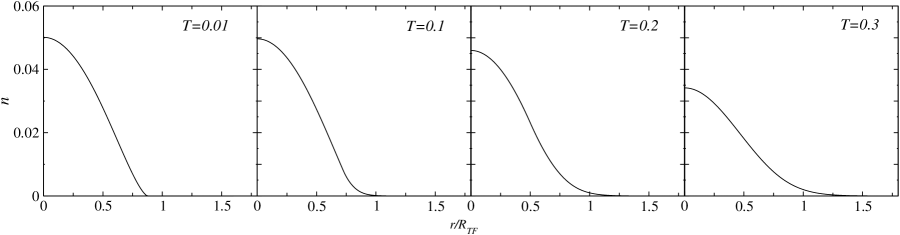
Figure 2: 3D density profiles $n(r)$ of a Fermi gas in a harmonic trap at unitarity at $T/T_{F}=0.01$, 0.1, 0.2, and $0.3$. The density distributions are smooth and monotonic, and become broader with $T$ increasing. There is no bimodal feature in the density profiles, in agreement with experimental observations. Here $T_{F}=E_{F}/k_{B}$ is the global Fermi temperature and $R_{TF}$ is the Thomas-Fermi radius. The density $n(r)$ is in units of $k_{F}^{-3}$.

At high enough $T$ in the BCS and unitary regimes, we sometimes find that there is no solution for $q_{cut}$ when $\Delta$ becomes small and $-\mu_{pair}$ becomes large. We then extrapolate $q_{cut}$ smoothly to zero at higher $T$ via $q_{cut}\propto\sqrt{\Delta}$. This avoids the unphysical abrupt shut down of the pseudogap at high $T$. In the BEC regime, however, one finds that $q_{cut}=+\infty$ and the pairs are bound and long lived, as expected physically.

VI Density Profiles

We now turn to include trap effects, with spherical trap potential $V_{ext}(r)=\frac{1}{2}m\omega^{2}r^{2}$. Within a trap, we impose the force balance equation, $-\nabla p=n\nabla V_{ext}$, where $p$ is the pressure and $V_{ext}$ is the trap potential. In the trap, the temperature is constant, so we have the relation $\nabla p=n\nabla\mu$. Thus we obtain $\nabla\mu=-\nabla V_{ext}(r)$, or

$$\mu(r)=\mu_{0}-V_{ext}(r)$$ (38)

where $\mu_{0}\equiv\mu(0)$ and $V_{ext}(0)=0$. This shows that the force balance condition naturally leads to the usual local density approximation (LDA) in which the fermionic chemical potential $\mu$ can be viewed as varying locally, but self consistently throughout the trap.

We can readily extend our self consistent equations to incorporate a trap, treated at the level of LDA. $T_{c}$ is defined as the highest temperature at which the self-consistent equations are satisfied precisely at the trap center. At a temperature $T$ lower than $T_{c}$ the superfluid region extends to a finite radius $R_{sc}$. The particles outside this radius are in a normal state, with or without a pseudogap. The important chemical potential $\mu_{pair}(r)$ is identically zero in the superfluid region $r<R_{sc}$ , and must be solved for self-consistently at larger radii. Our calculations proceed by numerically solving the self-consistent equations. In the figures below, we express length in units of the Thomas-Fermi radius $R_{TF}=\sqrt{2E_{F}/(m\omega^{2})}=2(3N)^{1/3}/k_{F}$; the density $n(r)$ and total particle number $N=\int d^{3}{\bf r}\,n(r)$ are normalized by $k_{F}^{3}$ and $(k_{F}R_{TF})^{3}$, respectively.

We determine $T_{c}$ as follows: (i) An estimated initial value for chemical potential is assigned to the center of the trap $\mu(0)$, which determines the local $\mu(r)=\mu(0)-V_{ext}(r)$. (ii) We solve the gap equation (1) and pseudogap equation (35) at the center (setting $\Delta_{pg}=\Delta$) to find $T_{c}$ and $\Delta(0,T_{c})$. (iii) We next determine the radius $R_{max}$ where $\Delta$ drops to zero. (iv) Next we solve the gap equation (34) and pseudogap equation (35) for $\Delta(r,T_{c})$ for $r\leq R_{max}$. Then $n(r)$ is determined using Eq. (36). (v) We integrate $n(r)$ over all space and enforce the total number constraint $N=\int d^{3}r\,n(r)$. We use nonlinear equation solvers which iteratively find the solution for the global $\mu(0)$ and the local gap parameters. Below $T_{c}$, an extra step is involved to determine the condensate edge, $R_{sc}$, where $\Delta_{sc}$ drops to zero. Within the superfluid core, Eqs. (1) and (35) are solved locally for $\Delta$ and $\Delta_{sc}$, with $\mu_{pair}(r)=0$.

VI.1 Numerical results for unpolarized case

In this section we address the particle density profiles at all $T$ in the near-BEC, the near-BCS, and the unitary regimes. For the latter this work helps establish why the measured density profiles appear to be so featureless. O’Hara et al. (2002); Bartenstein et al. (2004) Some time ago it was found O’Hara et al. (2002) that at unitarity the profiles were reasonably well described by a Thomas-Fermi (TF) fit at zero $T$, and in recent work Kinast et al. (2004) this procedure has been extended to finite temperatures, suggesting that it might be quite general. Our calculations indicate this TF fit is reasonably good below $T_{c}$, and becomes substantially better above $T_{c}$. The width of the profiles has been used to extract an effective temperature scale. Kinast et al. (2004) If we follow the same procedure Kinast et al. (2005) on our theoretical profiles we find that the temperature scale coincides with the physical $T$ quite precisely above $T_{c}$. Below $T_{c}$, because the condensate edge moves inwards as temperature increases, this tends to compensate for thermal broadening effects. In this way, in the superfluid phase the effective temperature needs to be recalibrated Kinast et al. (2005) to arrive at the physical temperature scale.

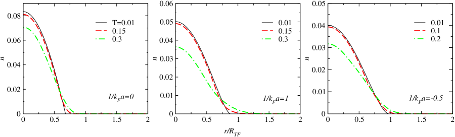
Figure 3: Comparison of 3D density profiles $n(r)$ at different temperatures between the unitary (left), near BEC ($1/k_{F}a=1$, middle) and near BCS ($1/k_{F}a=-0.5$, right panel) regimes. They broaden with increasing $T$ but shrink with increasing pairing strength.

Our work differs from previous theoretical studies Ho (2004); Chiofalo et al. (2002) by including the important effects of noncondensed pairs Stajic et al. (2004); Chen et al. (2005a) which are associated with pseudogap effects. These “bosons” are principally in the condensate region of the trap, whereas fermionic excitations tend to appear at the edge where the gap is small. In contrast to the work of Refs. Perali et al., 2004b and Perali et al., 2004a, our density profiles are monotonic in temperature and show none of the sharp features in the BEC which were predicted Perali et al. (2004a) from a generalization of the Nozieres–Schmitt-Rink approach. Our calculations show that pseudogap effects are responsible, not only for the relatively featureless density profiles we find in the unitary regime, but also for the behavior of the associated temperature evolution.

Figure 2 shows the behavior of the three-dimensional (3D) density profiles of a Fermi gas at unitarity as temperature progressively increases (from left to right). One can see that the profiles become progressively broader with increasing $T$. Because there is no bi-modality or other reflections of the condensate edge, one can thereby understand why the Thomas-Fermi fits are not inappropriate. A more quantitative comparison of this unitary case with experiment is in Ref. Stajic et al., 2005.

In Fig. 3 we present a comparison of the density profiles in a unitary system with the near BEC and near BCS cases. On the BEC side of resonance ($1/k_{F}a=1$) the profile is significantly narrower than that on the BCS side. The unitary case is somewhere in between. The quantity $\beta$ which is used in the literature to parameterize this width is of the order of $-0.41$ as compared with experiment where $\beta\approx-0.55$. Conventionally, $\beta$ is defined as the ratio of the attractive interaction energy to the kinetic energy and is given by $\mu=(1+\beta)E_{F}$ and $\mu_{0}=\sqrt{1+\beta}E_{F}$ for homogeneous and trapped unitary gases, respectively. The discrepancy between theory and experiment is associated with the absence of Hartree self-energy corrections in the BCS-Leggett mean field state. Thus, for more quantitative comparison with unitary experiments Stajic et al. (2005) we match the $\beta$ factor by going slightly on the BEC side of resonance.

VI.2 Numerical results for polarized case

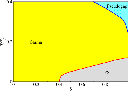
Figure 4: Phase diagram in the $T$-$\delta$ plane of a population imbalanced Fermi gas at $1/k_{F}a=1.5$ in the BEC regime. Here PS denotes phase separation, which exists only at low $T$ and high polarization.

In this section we show how the general shape of the density profiles at unitarity changes as one varies the polarization. Unlike the unpolarized case, we can identify features in the polarized gas profiles which indicate whether or not the gas is superfluid; these features are rather similar to what is observed experimentally. Zwierlein et al. (2006a); Partridge et al. (2006); Zwierlein et al. (2006b); Ric We also trace the evolution of the profiles from phase separation at low temperature to the Sarma phase.

We begin with Fig. 4 which shows the phase diagram at $1/k_{F}a=1.5$ on the BEC side of resonance. This should be compared with the counterpart phase diagrams for unitarity and the near-BCS which have been presented in Ref. Chien et al., 2007. The principal difference between unitarity and this case is that for the former the phase separation (PS) region is present at low $T$ over the entire range of polarizations, whereas in the BEC regime, it has been pushed toward the high polarization region of the phase diagram.

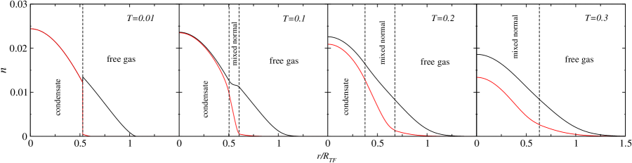
Figure 5: Evolution of the 3D density profiles $n(r)$ with temperature $T$ at unitarity and polarization $\delta=0.5$. The upper (black) and lower (red) curves are for the majority and minority species, respectively. From left to right, $T/T_{F}=0.01$, 0.1, 0.2, and 0.3. Phase separation occurs for $T/T_{F}=0.01$, where the profile shows abrupt changes at the phase boundary, whereas the Sarma phase prevails in the other cases so that the profiles are smooth. Bimodality is clearly visible in the Sarma cases. Within the vertical dashed lines there exists a paired normal region.

Figure 5 shows the temperature dependence of the unitary profiles for majority and minority spin components at $p=0.5$ for a range of temperatures, increasing from left to right. The lowest temperature ($T/T_{F}=0.01$) corresponds to a situation when phase separation is present, while the three higher temperature correspond to the Sarma phase. The condensate edge is clearly apparent in the phase separation scenario, with a jump in order parameter at the edge. For the Sarma phase cases, bimodality is clearly visible in the minority profile, and a kink-like feature is present in the majority profile well below $T_{c}$. At high $T$, both majority and minority profiles become closer to a Thomas-Fermi distribution, as polarization has penetrated into the superfluid core.

The vertical dashed lines for the three Sarma cases in the figure delimit the paired normal region. They correspond to the condensate edge, where $\Delta_{sc}$ drops to 0, and the gap edge where the total excitation gap $\Delta=\Delta_{pg}$ smoothly disappears. Between the two dashed lines the system is in a paired or highly correlated mixed normal state. Zwierlein et al. (2006b, a) The width of this mixed normal region grows with increasing temperature, and the condensate edge disappears above $T_{c}$. Outside the gap edge, the gas is free; there is a small range of $r$ where both spin components are present and a wider range where only the majority appears. In the phase separation regime, such a mixed normal region is essentially absent, Partridge et al. (2006); Ric and the condensate edge is indicated by a single dashed vertical line. For low $T$, we note that the condensate is essentially unpolarized.

In summary, in the phase separation regime, there are sharp discontinuities in the profile associated with the condensate edge, the other side of which is a free Fermi gas. In the Sarma phase, which is stabilized at higher T, there may also be indications of the condensate edge. Beyond the superfluid core, there is a highly correlated mixed normal region which carries a significant fraction of the polarization and is associated with the pseudogap phase. Finally, in the outer regime of the profile there is a free Fermi gas, which may consist of majority only or of both spin states. These three regions in the Sarma phase seem to be in accord with experiment. Zwierlein et al. (2006b, a) An important additional finding is that except at high temperatures the superfluid core seems to be robustly maintained at nearly zero polarization, as observed experimentally. Zwierlein et al. (2006a); Partridge et al. (2006); Zwierlein et al. (2006b); Ric

VII Thermodynamics

In this section we introduce Chen et al. (2005b) an approximate form for the thermodynamical potential (density), $\Omega$. We can, to a high level of accuracy, write this down analytically. It is important to assess this approximate form by studying various thermodynamical identities. We will do so here by checking Maxwell’s relations as well as establishing the relationship $p=\frac{2}{3}E$ between energy density $E$ and pressure $p$, which is expected Ho (2004); Thomas et al. (2005) to apply at strict unitarity. In the superfluid phase, we find there is essentially no deviation from the precise thermodynamical relations. Above $T_{c}$, we find deviations of from one to a few percent.

We begin with the unpolarized case. The quantity $\Omega$ is associated with a contribution from gapped fermionic excitations $\Omega_{f}$ as well as from non-condensed pairs, called $\Omega_{b}$. These two contributions are fully inter-dependent. The gap in the fermionic excitation spectrum is present only because there are pairs and conversely. We have

$$\Omega = \Omega_{f}+\Omega_{b}$$

$$\Omega_{f} = \Delta^{2}\chi_{0}+\sum_{\mathbf{k}}[(\xi_{\mathbf{k}}-E_{\mathbf{k}})-2T\ln(1+e^{-E_{\mathbf{k}}/T})],$$

$$\Omega_{b} = \sum_{\mathbf{q}}T\ln(1-e^{-\Omega_{\mathbf{q}}/T})\,.$$ (39)

where $\chi_{0}\equiv-U^{-1}-Z\mu_{pair}$. The pressure is simply

$$p=-\Omega$$ (40)

Here $\mu_{pair}=0$ at $T\leq T_{c}$, while above $T_{c}$ the superconducting order parameter $\Delta_{sc}=0$. Providing that we ignore the very weak dependence of the parameter $Z$ and the pair mass $M^{*}$ on $\Delta$, $\mu$ and $h$, we are able to derive our self consistent gap, pseudogap and number equations variationally. These self-consistent (local) equations are given by

$$\frac{\partial\Omega}{\partial\Delta}=0$$ (41)

which represents the gap equation (34). Similarly, we have

$$\frac{\partial\Omega}{\partial\mu_{pair}}=0$$ (42)

which leads to the equation for the pseudogap given by Eq. (35). Finally, the number equation

$$n=-\frac{\partial\Omega}{\partial\mu}$$ (43)

which yields Eq. (36). In a trap, this is subject to the total number constraint $N=\int d^{3}r\,n(r)$.

From the above thermodynamical potential, we can determine all other thermodynamic quantities. The energy (density) is

$$E = E_{f}+E_{b}$$

$$E_{f} = -\Delta^{2}\chi_{0}+\sum_{\mathbf{k}}[(\xi_{\mathbf{k}}-E_{\mathbf{k}})-2E_{\mathbf{k}}f(E_{\mathbf{k}})]+\mu n,$$

$$E_{b} = \sum_{\mathbf{q}}\Omega_{\mathbf{q}}b(\Omega_{\mathbf{q}}-\mu_{pair})\,.$$ (44)

and the entropy (density) is

$$S = S_{f}+S_{b}$$

$$S_{f} = 2\sum_{\mathbf{k}}\left[\frac{E_{\mathbf{k}}}{T}f(E_{\mathbf{k}})+\ln(1+e^{-E_{\mathbf{k}}/T})\right],$$

$$S_{b} = \sum_{\mathbf{q}}\left[\frac{\Omega_{\mathbf{q}}}{T}b(\Omega_{\mathbf{q}})+\ln(1-e^{-\Omega_{\mathbf{q}}/T})\right].$$ (45)

It is easy to verify the relation

$$\Omega_{f}=E_{f}-TS_{f}-\mu n$$ (46)

and

$$\Omega_{b}=E_{b}-TS_{b}-\mu_{pair}n_{pair}$$ (47)

with $n_{pair}=Z\Delta_{pg}^{2}$.

In the actual calculations of thermodynamic properties we combine Eq. (39) with a microscopic calculation of the non-condensed pair propagator, thereby determining $Z$, and $\Omega_{q}$ from the expansion of the inverse T-matrix. We test the validity, then, of our expression for the thermodynamic potential $\Omega$ by examining Maxwell identities. Indeed the deviation is generally at most at the few percent level, as will be illustrated below.

Finally, we end our analytical discussion with expressions for a polarized gas. Here the thermodynamical potential is given by

$$\Omega = \Omega_{f}+\Omega_{b}$$

$$\Omega_{f} = \Delta^{2}\chi_{0}+\sum_{\mathbf{k}}(\xi_{\mathbf{k}}-E_{\mathbf{k}})-\sum_{k,\sigma}T\ln(1+e^{-E_{k,\sigma}/T}),$$

$$\Omega_{b} = \sum_{\mathbf{q}}T\ln(1-e^{-\Omega_{\mathbf{q}}/T})\,.$$ (48)

Competing with this phase is the free Fermi gas phase which has thermodynamical potential density

$$\Omega_{free}=-T\sum_{\mathbf{k},\sigma}\ln{\left(1+e^{-\xi_{k\sigma}/T}\right)}$$ (49)

Here $E_{\mathbf{k}\sigma}=E_{\mathbf{k}}\mp h$ and $\xi_{\mathbf{k}\sigma}=\xi_{\mathbf{k}}\mp h$ for spin $\sigma=\uparrow,\downarrow$, respectively,

It should be noted that in this paper, we are concerned with primarily the internal energy (density) and pressure without the contribution from the external trap potential, in order to test the relationship $p/E=2/3$. The internal energy can be obtained by substituting for the chemical potential the local $\mu(r)$ in the term $E_{f}$ in Eq. (44). The total energy, which includes the trap potential, may be obtained by further adding $nV_{ext}(r)$ to $E_{f}$ in Eq. (44). For a harmonic trap at unitarity, the internal energy and the external trap potential energy are equal. Thomas et al. (2005)

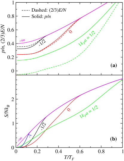
Figure 6: Thermodynamic behavior of a homogeneous Fermi gas at different $1/k_{F}a$ as labeled. Shown in (a) the comparison between per-particle energy (multiplied by 2/3, dashed lines) $(2/3)E/N$ and pressure $p/n$ (solid lines) and in (b) the entropy per particle $S/Nk_{B}$. Here $N=n$ since we have set volume $V=1$.

VII.1 Numerical Results for unpolarized case

In this section we discuss numerical results for thermodynamic properties principally for trapped Fermi gases within the unitary, near-BCS and near-BEC regimes. We find that unpaired fermions at the edge of the trap, where $\Delta$ is small, provide the dominant contribution to thermodynamical variables such as $E$ and $S$ at all but the lowest $T$. In addition to the usual gapped fermionic excitations, there are “bosons” which correspond to finite momentum pairs. Above $T_{c}$ these “bosons” lead to a normal state fermionic excitation gap (or “pseudogap”). Stajic et al. (2004); Chen et al. (2005a); Chin et al. (2004); Greiner et al. (2005) They are dominant only at very low $T\ll T_{c}$, leading to $S\propto T^{3/2}$. We emphasize that the normal state of these superfluids is never an ideal Fermi gas, except in the extreme BCS limit, or at sufficiently high $T$ above the pseudogap onset temperature $T^{*}$.

In Fig. 6, we plot (a) the energy per-particle $E/N$ (dashed lines) multiplied by 2/3 and pressure $p/n$ (solid lines) and (b) the entropy $S/Nk_{B}$ for a homogeneous system and for a range of values of $1/k_{F}a$, from noninteracting ($1/k_{F}a=-\infty$) to near BEC ($1/k_{F}a=1/2$). It can be seen that all curves approach the free Fermi gas results at $T>T^{*}$. It is also clear that, as expected, the energy and entropy are lowered as the system goes deeper into the BEC. The pairing onset temperature $T^{*}$ stands out in the figure as the most apparent temperature scale. We find virtually no thermodynamic feature at $T_{c}$. A small feature should be present in the BEC, becoming larger as the BCS regime is approached. This would appear if we included lifetime effects associated with the non-condensed pairs; in order to make the calculations manageable, we have ignored this complexity which has been addressed elsewhere. Chen et al. (2000) It should be stressed that $T^{*}$ represents a crossover temperature and is not to be associated with singular structure in thermodynamical variables, unlike $T_{c}$.

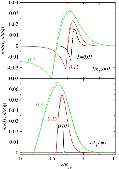
Figure 7: Test of Maxwell relations. The solid and dashed curves are $dn/dT$ and $ds/d\mu$, respectively, as function of trap radius, at different temperatures for $1/k_{F}a=0$ (upper) and $1/k_{F}a=1$ (lower panel). As labeled, the black, red and green colors correspond to $T/T_{F}=0.01$, 0.15, and 0.3, respectively. The difference between the solid and dashed curves, while largest in the normal regime, is almost negligible.

The comparison between the dashed and solid lines in Fig. 6(a) represents an important indicator of the universality expected at strict unitarity, where the energy density and pressure satisfy $p=\frac{2}{3}E$. Indeed the two curves are virtually indistinguishable in the superfluid phase at unitarity, and remain very close to each other in the normal phase. This relationship also holds for the non-interacting gas. By contrast, on the BEC side of resonance this relation is seriously violated, as expected.

Figure 7 represents a test of one particular Maxwell relation for the unitary case (upper panel) and for the near-BEC ($1/k_{F}a=1$, lower panel). Here we compare $dn/dT$ (solid lines) with $ds/d\mu$ (dashed lines). The horizontal axis is the trap radius in units of $R_{TF}$. At the lowest temperature this Maxwell relation is very well satisfied. The feature shown in the plotted derivatives corresponds to the condensate edge. As the temperature is raised the deviation is slight, but perceptible. The small breakdown in the Maxwell relations corresponds to our approximate treatment of the normal phase as discussed in Sec. IV.

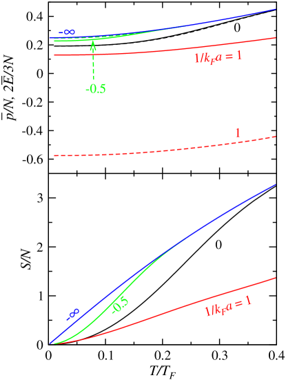
Figure 8: Trap averaged (per-particle) pressure $\bar{p}/N$ (solid), and internal energy $\bar{E}/N$ in the upper panel and entropy $S/N$ in the lower panel as a function of $T$ for $1/k_{F}a=-0.5$, 0, and 1, as labeled. The relation $p=2E/3$ is satisfied for and only for the unitary case. The agreement is nearly perfect at $T<T_{c}$. In the pseudogap phase, the discrepancy remains very small ($<5\%$). Here the contribution from the external trap potential is not included in the $\bar{p}$ or $\bar{E}$. $Tc/T_{F}=0.19$, 0.28, and 0.33, respectively, for the three regimes.

In Fig. 8 we plot the trap averaged pressure (per particle) $p/N$ (solid) and $(2/3)E/N$ (dashed lines) in the upper panel as well as entropy $S/N$ in the lower panel, as a function of temperature. For each quantity, the three curves correspond to unitarity and near-BCS ($1/k_{F}a=-0.5$) and near-BEC ($1/k_{F}a=1$), respectively, as labeled. As for the homogeneous case in Fig. 6, the closer the system is to BEC the lower the energy and entropy, as expected. Although not shown here, all curves will approach the free Fermi gas curve at sufficiently high $T$, corresponding to their respective $T^{*}$. By comparing the solid and dashed lines in the upper panel, one can see that the relation $p=2E/3$ is essentially satisfied at unitarity.

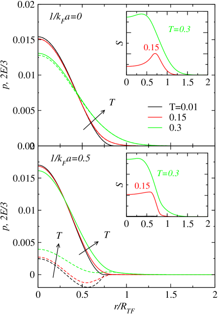
Figure 9: Spatial profile of the pressure $p(r)$ (solid) and internal energy $(2/3)E(r)$ (dashed lines) in the main figures as well as the entropy $S(r)$ in the insets at $T/T_{F}=0.01$ (black), 0.15 (red), and 0.3 (green curves), for the unitary (upper panel) and near BEC (lower panel), respectively. The arrows point in the direction of increasing $T$. At unitarity, the relation $p=2E/3$ is nearly perfect for the low $T$ profiles, while in the pseudogap phase, the deviation is less than 5%. The $1/k_{F}a=0.5$ case clearly violates the $p=2E/3$ relation.

Figure 9 plots the spatial distribution of the pressure $p$ (solid) and the energy $2E/3$ (dashed lines), as well as the entropy $S$ (inset) for three different temperatures, for the unitary (upper panel) and the near BEC ($1/k_{F}a=1/2$, lower panel) cases, respectively. The relation $p/E=2/3$ holds very well at unitarity for all temperatures shown, but, as expected, it is clearly violated in the near BEC case. For $1/k_{F}a=1/2$, one sees that the energy becomes negative at intermediate trap radii. This reflects the fact that at these radii, the density is reduced so that the local quantity $1/k_{F}a$ is effectively increased and the gas is in the BEC regime. At unitarity the entropy in the inset tends to peak towards the trap edge; this reflects the contribution from free fermions. By contrast these free fermions are relatively absent in the near-BEC case and the entropy is dominated by pair excitations leading to a relatively constant dependence on the trap radius.

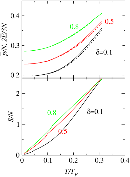
Figure 10: Temperature dependence of the trap averaged pressure $\bar{p}/N$ (solid), internal energy $\bar{E}/N$ (dashed) in the upper panel and entropy $S/N$ in the lower panel in a trap at unitarity for polarization $\delta=0.1$ (black), 0.5 (red), and 0.8 (green curves), as labeled. The $p=2E/3$ relation is satisfied at unitarity even with population imbalance. The small kink in $S/N$ indicates the change from phase separation to Sarma state. $T_{c}/T_{F}=0.28,0.25,0.19$ for polarization $\delta=0.1$, 0.5, and 0.8, respectively.

VII.2 Numerical results for polarized case

In this section we discuss the behavior of thermodynamical variables for a polarized gas at unitarity. In the upper panel of Fig. 10 we compare the trap averaged pressure per particle, $p/N$ (solid curves) and energy $(2/3)E/N$ (dashed curves) as a function of temperature, for three different polarizations $\delta=0.1$, 0.5, and 0.8. The lower panel shows the corresponding behavior of the entropy $S/N$. The figure illustrates that the lower the polarization the lower is the energy and entropy. This is because the system can take full advantage of the pairing when the polarization is small. Importantly, the upper panel demonstrates that the relation $p/E=2/3$ also appears to hold for a polarized gas. There are small kinks in the entropy curves at the two higher polarizations which reflect the transition from the phase separated to Sarma state.

The spatial profiles of the three thermodynamical variables are plotted for three different temperatures in Fig. 11 at fixed polarization $\delta=0.5$. The results are not dramatically different from the unpolarized case shown in the upper panel of Fig. 9. One can see that the $p/E=2/3$ relation holds rather well across the trap and that at intermediate temperatures, the entropy tends to peak somewhat inside the trap edge, reflecting the excitations of nearly free fermions in this regime.

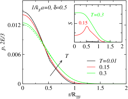
Figure 11: Spatial profiles of pressure (solid) and energy (dashed) in the main figure and entropy in the inset at unitarity and polarization $\delta=0.5$, for $T/T_{F}=0.01$ (black), 0.15 (red), and 0.3 (green curves), respectively. The black, red and green curves correspond to $T=0.01,0.15,0.3T_{F}$, respectively. The arrow points along the direction of increasing $T$. The $p=2E/3$ relation is essentially perfect for low $T$ profiles, and the deviation remains very small ($<5\%$) in the pseudogap phase.

VIII Superfluid Density

An essential component of any theory for BCS-BEC crossover is establishing that the superfluid density is well behaved. The superfluid density $n_{s}(T)$ is perhaps the best reflection of a proper (or improper) description of the superfluid phase. This meaningful description is not at all straightforward to come by once one includes self energy corrections to the BCS gap and number equation. These two must be treated on an equal footing in order for the “diamagnetic” and “paramagnetic currents” to precisely cancel at $T_{c}$ when approached from below. (And the $T_{c}$ that one computes from below has to be the same as that computed from the pairing instability of the normal phase).

This cancellation of diamagnetic and paramagnetic currents is deeply and importantly related to generalized Ward identities as we will show below. These arise from a connection between the one particle properties (which show up in the diamagnetic current, through the number equation) and the two particle properties (which, for example, reflect the fermionic excitation spectrum $E_{\mathbf{k}}$ and show up in the gap equation). It is important to stress at the outset that because we must distinguish between the gap and the order parameter, there is no unambiguous way to make use of the Nambu Gor’kov formalism. One can readily see, however, that the combination $GG_{0}$ is, in effect, proportional to that Gor’kov “F” function which involves the full excitation gap $\Delta$, rather than the order parameter.

Whether one considers a charged or an uncharged system, the formal analysis is the same. Here for the sake of definiteness we refer to a charged superconductor. We consider the in-plane penetration depth kernel $K(0)$ in linear response theory. Within the transverse gauge we may write down this response without including the contribution from collective modes. The London penetration depth is $\lambda^{-2}_{L}=\mu_{0}e^{2}(n_{s}/m)$, where $\mu_{0}$ is the magnetic permitivity. Here we set $\mu_{0}=e=1$ for convenience. From linear response theory,

$$\lambda^{-2}_{L}=K_{xx}(0)=\left(\frac{n}{m}\right)_{xx}-P_{xx}(0)\>,$$ (50)

where $K$ is defined by

$$J_{\mu}(Q)=P_{\mu\nu}A_{\nu}(Q)-\left(\frac{n}{m}\right)_{\mu\nu}\!A_{\nu}(Q)=-K_{\mu\nu}(Q)A_{\nu}(Q)\>,$$ (51)

and the current-current correlation function

$$P_{\mu\nu}(Q)=\int_{0}^{\beta}\>d\tau\>e^{i\Omega_{n}\tau}\langle j_{\mu}({\mathbf{q}},\tau)j_{\nu}(-{\mathbf{q}},0)\rangle$$

$$= -2\mathop{\sum_{K}}{\Lambda}_{\mu}(K,K+Q)G(K+Q){\lambda}_{\nu}(K+Q,K)G(K)\>.$$

Here we use the four-vector notation, $A_{\mu}=(\phi,\mathbf{A})$, $j_{\mu}=(\rho,\mathbf{j})$, and the bare vertex $\lambda_{\mu}=(1,\bm{\lambda})$. Summation is assumed on repeated indices, with the convention $A_{\mu}B_{\mu}=A_{0}B_{0}-\mathbf{A}\cdot\mathbf{B}$. Without loss of generality we can ignore collective mode effects and work in a transverse gauge.

For the bare vertex, we have $\lambda_{0}=1$ and

$$\bm{\lambda}(K,K+Q)=\vec{\nabla}_{\mathbf{k}}\epsilon_{{\mathbf{k}}+{\mathbf{q}}/2}=\frac{1}{m}\left({\mathbf{k}}+\frac{{\mathbf{q}}}{2}\right)\>,$$ (53)

The electromagnetic vertex can be written in terms of the corrections coming from the two self-energy components as

$$\Lambda=\lambda+\delta\Lambda_{pg}+\delta\Lambda_{sc}\>,$$ (54)

where $\delta\Lambda_{pg}$ is the pseudogap term. This contribution deriving from pair fluctuations contains terms associated with Maki-Thompson (MT) like diagrams as well as Aslamazov-Larkin terms (AL) which appear in the theory of conventional superconducting fluctuations. Here the situation is somewhat more complex because of the appearance of one dressed and one bare Green’s function in the pair propagator, which leads to two AL diagrams. As a result the AL term itself depends on a (gauge covariant) vertex function $\Lambda^{\prime}$. We may write

$$\delta\Lambda_{pg}\equiv\delta\Lambda_{MT}+\delta\Lambda_{AL_{1}}+\delta\Lambda_{AL_{2}}(\Lambda^{\prime})\>.$$ (55)

The diagrams contributing to the full electromagnetic vertex $\Lambda$ in the transverse gauge are given in Fig. 12. Here $\Lambda_{MT}$ is given by the $MT_{pg}$ diagram, and $\delta\Lambda_{sc}$ is given by the $MT_{sc}$ diagram. In contrast to the electromagnetic vertex $\Lambda$, the gauge covariant vertex $\Lambda^{\prime}$ satisfies a generalized Ward identity to be discussed below.

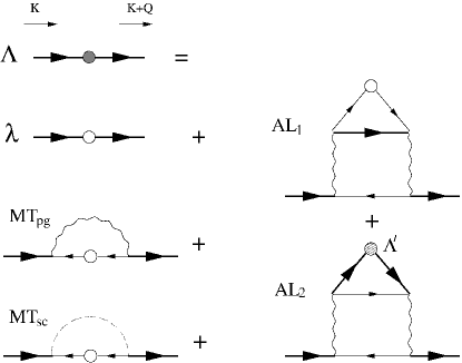
Figure 12: Diagrams contributing to the full electromagnetic vertex ${\Lambda}$ in the transverse gauge. Here the wiggly lines represent the $T$-matrix $t_{pg}$ and the dashed line represent the singular “condensate propagator” $t_{sc}$, both shown in Fig. 1. The gauge covariant full vertex ${\Lambda}^{\prime}$ contains the electromagnetic vertex insertion along $t_{sc}$.

We now show that there is a precise cancellation between the $MT_{pg}$ and $AL_{1}$ pseudogap diagrams at $Q=0$. This cancellation follows directly from a generalized Ward identity (GWI)

$$Q\cdot\lambda(K,K+Q)=G_{0}^{-1}(K)-G_{0}^{-1}(K+Q)\>,$$ (56)

which can be shown to imply

$$Q\cdot[\delta\Lambda_{AL_{1}}(K,K+Q)+\delta\Lambda_{MT}(K,K+Q)]=0$$ (57)

so that $\delta\Lambda_{AL_{1}}(K,K)=-\delta\Lambda_{MT}(K,K)$ is obtained exactly from the $Q\rightarrow 0$ limit of the GWI.

To see this explicitly note that

$$\delta{\Lambda}_{MT}^{\mu} = -\sum_{P}t(P)G_{0}(-K-Q+P)$$ (58)

$$\times{\lambda}^{\mu}(-K-Q+P,-K+P)$$

$$\times G_{0}(-K+P)$$

Similarly we have

$$\delta{\Lambda}_{AL_{1}}^{\mu} = -\sum_{P}G_{0}(-K+P)t(P+Q)$$ (59)

$$\times\Big{\{}\sum_{K^{\prime}}G(-K^{\prime}+P)G_{0}(K^{\prime}+Q)$$

$$\times{\lambda}_{\mu}(K^{\prime}+Q,K^{\prime})G_{0}(K^{\prime})\Big{\}}t(P)$$

We may write

$$t(P)^{-1}=U^{-1}-\sum_{K_{1}}G(K_{1}+P)G_{0}(-K_{1})$$ (60)

Then combining terms

$$Q\cdot(\delta{\Lambda}_{MT}+\delta{\Lambda}_{AL_{1}})=\sum_{P}t(P)G_{0}(-K+P)\\ \times\Big{\{}G_{0}(-K-Q+P)[G_{0}^{-1}(P-K)-G_{0}^{-1}(P-K-Q)]\\ -t(P+Q)\sum_{K^{\prime}}G(-K^{\prime}+P)G_{0}(K^{\prime}+Q)G_{0}(K^{\prime})\\ \times[G_{0}^{-1}(K^{\prime})-G_{0}^{-1}(K^{\prime}+Q)]\Big{\}}$$ (61)

It then follows using Eq. (60) that this equation vanishes and we have proved the desired relation between the Maki-Thompson vertex and the $AL_{1}$ vertex.

The GWI is not to be imposed on ${\Lambda}$ since we are evaluating the electrodynamic response in a fixed (transverse) gauge. However, the full gauge covariant internal vertex ${\Lambda}^{\prime}$ is consistent with the GWI. This internal vertex ${\Lambda}^{\prime}$ then satisfies

$$Q\cdot{\Lambda}^{\prime}(K,K+Q)=G^{-1}(K)-G^{-1}(K+Q)\,.$$ (62)

The above result can be used to infer a relation analogous to Eq. (57) for the $AL_{2}$ diagram: so that $\delta{\Lambda}_{AL_{2}}(K,K)=-\delta{\Lambda}_{MT}(K,K)$. More generally

$$Q\cdot(\delta\Lambda_{AL1}+\delta\Lambda_{AL2})=-2Q\cdot\delta{\Lambda}_{MT},$$ (63)

Therefore the combination of these three diagrams (in conjunction with Eq. (55)) leads to

$$Q\cdot\delta{\Lambda}_{pg}(K,K)=-Q\cdot\delta{\Lambda}_{MT}(K,K)\>,$$ (64)

which expresses this pseudogap contribution to the vertex entirely in terms of the Maki-Thompson diagram shown in the figure. One can show explicitly that

$$\delta{\Lambda}^{\mu}_{MT}(K,K)=-\frac{\partial\Sigma_{pg}(K)}{\partial k_{\mu}}\>.$$ (65)

This can be proved as follows. We write

$$Q\cdot\delta{\Lambda}_{MT}=-\sum_{P}t_{pg}(P)[G_{0}(-K+P)-G_{0}(-K-Q+P)],$$ (66)

where we have used the GWI involving the bare Green’s functions to eliminate ${\lambda}$. Now taking the $\mathbf{q}=0$ limit with $\omega=0$ and using Eq. (64) and the expression of $\Sigma_{pg}(K)$ we arrive at Eq. (65).

Combining terms we find

$$\delta{\Lambda}^{\mu}_{pg}(K,K)=\frac{\partial\Sigma_{pg}(K)}{\partial k_{\mu}}\>,$$ (67)

This demonstrates consistency; that is, the usual Ward identity applies to the pseudogap contribution.

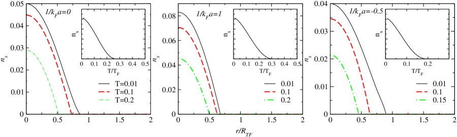
Figure 13: Spatial profiles of superfluid density at zero polarization at different temperatures (as labeled) for $1/k_{F}a=0$ (left), 1 (middle), and -0.5 (right panel). The insets show the $T$-dependence of trap integrated superfluid density. All the profiles are smooth, single-valued, and monotonic, evolving continuously with radius and temperature.

Now we turn to the superconducting vertex contributions. As can be seen by a simple inspection of the diagrams, the superconducting contribution is closely analogous to Eq. (65) so that we have

$$\delta{\Lambda}^{\mu}_{sc}(K,K)=-\frac{\partial\Sigma_{sc}(K)}{\partial k_{\mu}}\>.$$ (68)

Importantly, the above equation contains a sign change (as compared with Eq. (67)). This is associated with the transverse gauge and violates the Ward identity. It is central to the existence of a Meissner effect. The fact that the pseudogap contributions are consistent with generalized Ward identities is an important aspect of the present calculations. This implies that there is no direct Meissner contribution associated with the pseudogap self-energy.

We next explicitly evaluate the superfluid density using Eq. (50). For this purpose, we only need the spatial components of the vertex functions. Note that the pseudogap contribution to $(n_{s}/m)$ drops out by virtue of Eq. (67). The density can be rewritten using integration by parts,

$$\left(\frac{n}{m}\right)_{\alpha\beta} = 2\sum_{K}\frac{\partial^{2}\epsilon_{\mathbf{k}}}{\partial k_{\alpha}\partial k_{\beta}}G(K)=-2\sum_{K}\frac{\partial\epsilon_{\mathbf{k}}}{\partial k_{\alpha}}\frac{\partial G(K)}{\partial k_{\beta}}$$

$$= -2\sum_{K}G^{2}(K)\frac{\partial\epsilon_{\mathbf{k}}}{\partial k_{\alpha}}\left(\frac{\partial\epsilon_{\mathbf{k}}}{\partial k_{\beta}}+\frac{\partial\Sigma_{pg}}{\partial k_{\beta}}+\frac{\partial\Sigma_{sc}}{\partial k_{\beta}}\right)\>,$$

where $\alpha,\beta=1,2,3$. Note here the surface term vanishes in all cases. The superfluid density is given by

$$\frac{n_{s}}{m}=2\sum_{K}G^{2}(K)\frac{\partial\epsilon_{\mathbf{k}}}{\partial k_{x}}\bigg{[}\delta{\Lambda}_{sc}(K,K)_{x}-\frac{\partial\Sigma_{sc}(K)}{\partial k_{x}}\bigg{]}\>.\$$ (70)

Equation (70) can be readily evaluated using the superconducting vertex and the superconducting self-energy $\Sigma_{sc}(K)=-\Delta_{sc}^{2}G_{0}(-K)$ associated with our $GG_{0}$-based T-matrix approach. In addition, we introduce an approximation in our evaluation of $G$ via Eq. (18), to find

$$\left(\frac{n_{s}}{m}\right)=2\sum_{{\mathbf{k}}}\frac{\Delta_{sc}^{2}}{E_{\mathbf{k}}^{2}}\left[\frac{1-2f(E_{\mathbf{k}})}{2E_{\mathbf{k}}}+f^{\prime}(E_{\mathbf{k}})\right]\left(\frac{\partial\epsilon_{\mathbf{k}}}{\partial k_{x}}\right)^{2}.$$ (71)

More generally, we can define a relationship

$$\left(\frac{n_{s}}{m}\right)=\frac{\Delta_{sc}^{2}}{\Delta^{2}}\left(\frac{n_{s}}{m}\right)^{BCS}\>,$$ (72)

where $(n_{s}/m)^{BCS}$ is just $(n_{s}/m)$ with the overall prefactor $\Delta_{sc}^{2}$ replaced with $\Delta^{2}$ in Eq. (71). Obviously, in the pseudogap phase, $(n_{s}/m)^{BCS}$ does not vanish at $T_{c}$.

Finally, in the polarized case it can be shown that the superfluid density is given by Eq. (71) with the Fermi function and its derivative replaced by the quantities $\bar{f}$ and $\bar{f^{\prime}}$, respectively.

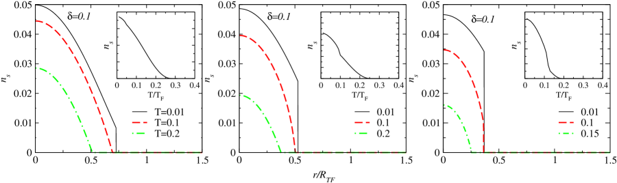
Figure 14: Spatial profiles of superfluid density at unitary at different temperatures (as labeled) for polarization $\delta=0.1$, 0.5, and 0.8 from left to right. The insets show the trap integrated superfluid density as function of $T$. High $T$ profiles are in the Sarma phase, and therefore, smooth, evolving continuously with radius. In contrast, The lowest $T$ curves are in the phase separation regime and thus show an abrupt drop. The kinks in the trap integrated $n_{s}$ reflect the transition from phase separation to Sarma state.

VIII.1 Numerical results for unpolarized and polarized cases

The behavior of the superfluid density $n_{s}(T)$ is viewed as one of the important indicators of the quality of a given BCS-BEC crossover theory. Plots of $n_{s}(T)$ in Ref. Andrenacci et al., 2003 stop at about $T_{c}/2$, above which it is argued that the calculations are unreliable. Alternative plots Gri show double-valued functions, particularly on the BEC side of resonance. While $n_{s}(T)$ is not explicitly evaluated, it will necessarily exhibit a first order transition in the work of Ref. Haussmann et al., 2007.

It is important, then, to show that $n_{s}(T)$ corresponds to the appropriate physical behavior in the current theory. First, we present results for unpolarized Fermi gases. The spatial distributions of $n_{s}(r)$ in a trap are plotted in Fig. 13 for different temperatures and three different scattering lengths ranging from near BCS to unitary to near BEC. In the insets are plotted the temperature dependence of the trap integrated superfluid density. All curves are well behaved, single-valued, and monotonic from $T=0$ to $T=T_{c}$. The superfluid density vanishes precisely at $T_{c}$.

Analogous plots are shown in Fig. 14 for a polarized gas in the unitary case and at three different polarizations $\delta=0.1$, 0.5, and 0.8. The main figures present plots as a function of trap radius, whereas the insets are plots as a function of temperature. Here, by contrast, the behavior is not always smooth. These sharp features are all expected and associated with polarization effects. At the lowest temperatures in the main body of each of these figures one can see the effects of phase separation on $n_{s}$. The superfluid density stops abruptly at the interface between the normal and superfluid. At higher $T$ in the Sarma phase, the curves end continuously at the trap edge. At the higher two polarizations the two insets indicate kinks which reflect the transition from a phase separated to a Sarma phase.

IX Conclusions

There are many different renditions of BCS-BEC crossover physics in the literature, but what has guided us here is the implementation of a sound methodology for characterizing three fundamental properties: thermodynamics, density profiles and superfluid density with and without population imbalance. While there is considerable emphasis in the literature on numerical precision one goal of this paper was to set up a different set of criteria against which theories as well as simulations can be checked. Monte Carlo simulations are sometimes argued Bulgac et al. (2006) to be the ultimate theory. While they may provide reliable numbers, these alone (in the absence of more analytic many body schemes) will not yield sufficient insight into the complex physics of these very anomalous superfluids.

Four important and inter-related physical properties were emphasized here. (i) There must be a consistent treatment of “pseudogap” effects. That is, the fermionic excitation spectrum, $E_{\mathbf{k}}$ must necessarily be modified from the usual BCS form. Here, based on a systematic analysis, we implement this modification by replacing the order parameter with the total excitation gap $\Delta$. (ii) The theory must lend itself to a consistent description of the superfluid density $n_{s}(T)$ from zero to $T_{c}$. The quantity $n_{s}(T)$ should be single valued and monotonic.NsF It must necessarily disappear at the same $T_{c}$ one computes from the normal state instability; $n_{s}(T)$ is at the heart of a proper description of the superfluid phase. (iii) The behavior of the density profiles, which are at the basis for all thermodynamical calculations of trapped Fermi gases, must be compatible with experiment. Near and at unitarity, they are relatively smooth and featureless, well fit to a Thomas-Fermi like form. Only in the presence of polarization effects can one use these unitary profiles to find signatures of the condensate edge. (iv) The thermodynamical potential $\Omega$ should be variationally consistent with the gap and number equations. It should satisfy appropriate Maxwell relations and at unitarity be compatible with the constraint relating the pressure $p$ to the energy density: $p=\frac{2}{3}E$. Here we find this to be the case for a population imbalanced gas as well to the same level of numerical precision as for an unpolarized gas.

For semi-quantitative comparisons with experiment there have been notable successes within the present theoretical framework which address a very wide group of experiments, including polarized and unpolarized gases. Kinast et al. (2005); Stajic et al. (2005); Chien et al. (2007); Chen et al. (2006b, c); He et al. (2005); Levin and Chen However, it is clear that detailed quantitative agreement is not always possible. Altmeyer et al. (2007) The calculated $\beta$ factor at unitarity ($\beta=-0.41$), is not precise, as compared with experiment ($\beta\approx-0.55$). Moreover, the ratio of effective inter-boson scattering length to the fermionic scattering length is found to be 2.0, rather than 0.6. Petrov et al. (2004) Indeed, inter-boson effects are included only in a mean field sense at the level of the simple BCS-Leggett wave function and related T-matrix scheme. One knows Tan and Levin (2006) how to arrive at a more Bogoliubov-like treatment of the pairs which properly treats inter-boson effects appropriate to the deep BEC. It can be shown Tan and Levin (2006) to yield the factor $0.6$. This involves adding to the wave function additional terms involving four and six creation operators. However, there is no natural and tractable extension at unitarity.

We have emphasized here that what is most unique and interesting about these trapped Fermi gases lies not so much in the ground state, but rather in finite temperature phenomena. It is at finite $T$ that one sees a new form of fermionic superfluidity in which pair condensation and pair formation take place on distinctly different temperature scales. This temperature separation requires radical changes in the way we think about fermionic superfluidity, relative to our experience with strict BCS theory. We have argued here that at this relatively early stage of our understanding, it is more important to capture the central physics of this exotic superfluidity, than to arrive at precise numerical agreement with experiment. Ultimately we must do both, as has been possible for the Bose gases. Nevertheless assessing a theory based on understanding the qualitative physics has to proceed an assessment based on quantitative comparisons.

This work is supported by Grant Nos. NSF PHY-0555325 and NSF-MRSEC DMR-0213745.

References

- Leggett (2006) A. J. Leggett, Nature Physics 2, 134 (2006).
- Randeria (1995) M. Randeria, in Bose Einstein Condensation, edited by A. Griffin, D. Snoke, and S. Stringari (Cambridge Univ. Press, Cambridge, 1995), pp. 355–92.
- Chen et al. (2005a) Q. J. Chen, J. Stajic, S. N. Tan, and K. Levin, Phys. Rep. 412, 1 (2005a).
- (4) K. Levin and Q. J. Chen, e-print cond-mat/0611104.
- Eagles (1969) D. M. Eagles, Phys. Rev. 186, 456 (1969).
- Leggett (1980) A. J. Leggett, in Modern Trends in the Theory of Condensed Matter (Springer-Verlag, Berlin, 1980), pp. 13–27.
- Micnas et al. (1990) R. Micnas, J. Ranninger, and S. Robaszkiewicz, Rev. Mod. Phys. 62, 113 (1990).
- Pieri and Strinati (2005) P. Pieri and G. C. Strinati, Phys. Rev. B. 71, 094520 (2005).
- (9) To be precise, for a homogeneous Fermi gas with population imbalance, the superfluid density has been found to exhibit a nonmonotonic dependence on temperature in the unitary and BCS regimes. This leads to intermediate temperature superfluidity Chien et al. (2006b); Chen et al. (2006a). Nevertheless, it has been found to be monotonic in a trap.
- Ho (2004) T.-L. Ho, Phys. Rev. Lett. 92, 090402 (2004).
- Thomas et al. (2005) J. E. Thomas, J. Kinast, and A. Turlapov, Phys. Rev. Lett. 95, 120402 (2005).
- Nozières and Schmitt-Rink (1985) P. Nozières and S. Schmitt-Rink, J. Low Temp. Phys. 59, 195 (1985).
- Kosztin et al. (2000) I. Kosztin, Q. J. Chen, Y.-J. Kao, and K. Levin, Phys. Rev. B 61, 11662 (2000).
- Tan and Levin (2006) S. N. Tan and K. Levin, Phys. Rev. A 74, 043606 (2006).
- Pieri and Strinati (2003) P. Pieri and G. C. Strinati, Phys. Rev. Lett. 91, 030401 (2003).
- Chen et al. (1998) Q. J. Chen, I. Kosztin, B. Jankó, and K. Levin, Phys. Rev. Lett. 81, 4708 (1998).
- Micnas and Robaszkiewicz (1998) R. Micnas and S. Robaszkiewicz, Cond. Matt. Phys. 1, 89 (1998).
- Ranninger and Robin (1996) J. Ranninger and J. M. Robin, Phys. Rev. B 53, R11961 (1996).
- Perali et al. (2002) A. Perali, P. Pieri, G. C. Strinati, and C. Castellani, Phys. Rev. B 66, 024510 (2002).
- Milstein et al. (2002) J. N. Milstein, S. J. J. M. F. Kokkelmans, and M. J. Holland, Phys. Rev. A 66, 043604 (2002).
- Ohashi and Griffin (2002) Y. Ohashi and A. Griffin, Phys. Rev. Lett. 89, 130402 (2002).
- Ohashi and Griffin (2003) Y. Ohashi and A. Griffin, Phys. Rev. A 67, 063612 (2003).
- Pieri et al. (2004) P. Pieri, L. Pisani, and G. C. Strinati, Phys. Rev. Lett. 92, 110401 (2004).
- Trivedi and Randeria (1995) N. Trivedi and M. Randeria, Phys. Rev. Lett. 75, 312 (1995).
- Jankó et al. (1997) B. Jankó, J. Maly, and K. Levin, Phys. Rev. B 56, R11407 (1997).
- Chen et al. (1999) Q. J. Chen, I. Kosztin, B. Jankó, and K. Levin, Phys. Rev. B 59, 7083 (1999).
- Stajic et al. (2004) J. Stajic, J. N. Milstein, Q. J. Chen, M. L. Chiofalo, M. J. Holland, and K. Levin, Phys. Rev. A 69, 063610 (2004).
- Kadanoff and Martin (1961) L. P. Kadanoff and P. C. Martin, Phys. Rev. 124, 670 (1961).
- Chen (2000) Q. J. Chen, Ph.D. thesis, University of Chicago (2000), (unpublished).
- Fetter and Walecka (1971) A. L. Fetter and J. D. Walecka, Quantum Theory of Many-Particle Systems (McGraw-Hill, San Francisco, 1971).
- Baym (1962) G. Baym, Phys. Rev. 127, 1391 (1962).
- Vilk and Tremblay (1997) Y. M. Vilk and A. M. S. Tremblay, J. Phys I (France) 7, 1309 (1997).
- Tchernyshyov (1997) O. Tchernyshyov, Phys. Rev. B 56, 3372 (1997).
- Singer et al. (1997) J. M. Singer, M. H. Pedersen, and T. Schneider, Physica B 230, 955 (1997).
- Pedersen et al. (1997) M. H. Pedersen, J. J. Rodriguez-Nunez, H. Beck, T. Schneider, and S. Schafroth, Z. Phys. B 103, 21 (1997).
- Haussmann et al. (2007) R. Haussmann, W. Rantner, S. Cerrito, and W. Zwerger, Phys. Rev. A 75, 023610 (2007).
- Haussmann (1993) R. Haussmann, Z. Phys. B 91, 291 (1993).
- Perali et al. (2004a) A. Perali, P. Pieri, L. Pisani, and G. C. Strinati, Phys. Rev. Lett. 92, 220404 (2004a).
- Serene (1989) J. W. Serene, Phys. Rev. B 40, 10873 (1989).
- Dru (a) H. Hu, X. J. Liu, and P. D. Drummond, Phys. Rev. A73, 023617 (2006); Europhys. Lett. 74, 574 (2006).
- Dru (b) These same authors recently investigated an approach which uses a mix of and in the -matrix and obtained different results from the present work. It should be pointed out that they failed to include the noncondensed pair contribution in the gap equation.
- Perali et al. (2004b) A. Perali, P. Pieri, and G. C. Strinati, Phys. Rev. Lett. 93, 100404 (2004b).
- Petrov et al. (2004) D. S. Petrov, C. Salomon, and G. V. Shlyapnikov, Phys. Rev. Lett. 93, 090404 (2004).
- Pieri and Strinati (2006) P. Pieri and G. C. Strinati, Phys. Rev. Lett. 96, 150404 (2006).
- Brodsky et al. (2006) I. V. Brodsky, M. Y. Kagan, A. V. Klaptsov, R. Combescot, and X. Leyronas, Phys. Rev. A 73, 032724 (2006).
- Patton (1971) B. R. Patton, Ph.D. thesis, Cornell University (1971), (unpublished).
- Maly et al. (1999a) J. Maly, B. Jankó, and K. Levin, Physica C 321, 113 (1999a).
- Chien et al. (2006a) C.-C. Chien, Q. J. Chen, Y. He, and K. Levin, Phys. Rev. A 74, 021602(R) (2006a).
- Machida et al. (2006) K. Machida, T. Mizushima, and M. Ichioka, Phys. Rev. Lett. 97, 120407 (2006).
- Yi and Duan (2006) W. Yi and L. M. Duan, Phys. Rev. A 73, 031604(R) (2006).
- (51) G. B. Partridge, W. Li, Y. A. Liao, R. G. Hulet, M. Haque, and H. T. C. Stoof, Phys. Rev. Lett. 97, 190407 (2006).
- Sarma (1963) G. Sarma, J. Phys. Chem. Solids 24, 1029 (1963).
- Pao et al. (2006) C. H. Pao, S. T. Wu, and S. K. Yip, Phys. Rev. B 73, 132506 (2006).
- Sheehy and Radzihovsky (2006) D. E. Sheehy and L. Radzihovsky, Phys. Rev. Lett. 96, 060401 (2006).
- De Silva and Mueller (2006) T. N. De Silva and E. J. Mueller, Phys. Rev. Lett. 97, 070402 (2006).
- Haque and Stoof (2006) M. Haque and H. T. C. Stoof, Phys. Rev. A 74, 011602(R) (2006).
- Chien et al. (2006b) C.-C. Chien, Q. J. Chen, Y. He, and K. Levin, Phys. Rev. Lett. 97, 090402 (2006b).
- Chen et al. (2006a) Q. J. Chen, Y. He, C.-C. Chien, and K. Levin, Phys. Rev. A 74, 063603 (2006a).
- Parish et al. (2007) M. M. Parish, F. M. Marchetti, A. Lamacraft, and B. D. Simons, Nature Phys. 3, 124 (2007).
- (60) P. F. Bedaque, H. Caldas, and G. Rupak, Phys. Rev. Lett. 91, 247002 (2003); H. Caldas, Phys. Rev. A69, 063602 (2004).
- Chien et al. (2007) C.-C. Chien, Q. J. Chen, Y. He, and K. Levin, Phys. Rev. Lett. 98, 110404 (2007).
- Chen et al. (2007) Q. J. Chen, Y. He, C.-C. Chien, and K. Levin, Phys. Rev. B 75, 014521 (2007).
- (63) P. Fulde and R. A. Ferrell, Phys. Rev. 135, A550 (1964); A. I. Larkin and Y. N. Ovchinnikov, Zh. Eksp. Teor. Fiz. 47, 1136 (1964) [Sov. Phys. JETP 20, 762 (1965)].
- Maly et al. (1999b) J. Maly, B. Jankó, and K. Levin, Phys. Rev. B 59, 1354 (1999b).
- O’Hara et al. (2002) K. M. O’Hara et al., Science 298, 2179 (2002).
- Bartenstein et al. (2004) M. Bartenstein, A. Altmeyer, S. Riedl, S. Jochim, C. Chin, J. H. Denschlag, and R. Grimm, Phys. Rev. Lett. 92, 120401 (2004).
- Kinast et al. (2004) J. Kinast, A. Turlapov, and J. E. Thomas (2004), preprint cond-mat/0409283.
- Kinast et al. (2005) J. Kinast, A. Turlapov, J. E. Thomas, Q. J. Chen, J. Stajic, and K. Levin, Science 307, 1296 (2005), published online 27 January 2005; doi:10.1126/science.1109220.
- Chiofalo et al. (2002) M. L. Chiofalo, S. J. J. M. F. Kokkelmans, J. N. Milstein, and M. J. Holland, Phys. Rev. Lett. 88, 090402 (2002).
- Stajic et al. (2005) J. Stajic, Q. J. Chen, and K. Levin, Phys. Rev. Lett. 94, 060401 (2005).
- Zwierlein et al. (2006a) M. W. Zwierlein, A. Schirotzek, C. H. Schunck, and W. Ketterle, Science 311, 492 (2006a).
- Partridge et al. (2006) G. B. Partridge, W. Li, R. I. Kamar, Y. A. Liao, and R. G. Hulet, Science 311, 503 (2006).
- Zwierlein et al. (2006b) M. W. Zwierlein, C. H. Schunck, A. Schirotzek, and W. Ketterle, Nature (London) 442, 54 (2006b).
- Chen et al. (2005b) Q. J. Chen, J. Stajic, and K. Levin, Phys. Rev. Lett. 95, 260405 (2005b).
- Chin et al. (2004) C. Chin, M. Bartenstein, A. Altmeyer, S. Riedl, S. Jochim, J. Hecker-Denschlag, and R. Grimm, Science 305, 1128 (2004).
- Greiner et al. (2005) M. Greiner, C. A. Regal, and D. S. Jin, Phys. Rev. Lett. 94, 070403 (2005).
- Chen et al. (2000) Q. J. Chen, I. Kosztin, and K. Levin, Phys. Rev. Lett. 85, 2801 (2000).
- Andrenacci et al. (2003) N. Andrenacci, P. Pieri, and G. C. Strinati, Phys. Rev. B 68, 144507 (2003).
- (79) E. Taylor, A. Griffin, N. Fukushima, and Y. Ohashi, Phys. Rev. A74, 063626 (2006); N. Fukushima, Y. Ohashi, E. Taylor, and A. Griffin, Phys. Rev. A75, 033609 (2007).
- Bulgac et al. (2006) A. Bulgac, J. E. Drut, and P. Magierski, Phys. Rev. Lett. 96, 090404 (2006).
- Chen et al. (2006b) Q. J. Chen, C. A. Regal, M. Greiner, D. S. Jin, and K. Levin, Phys. Rev. A 73, 041601 (2006b).
- Chen et al. (2006c) Q. J. Chen, C. A. Regal, D. S. Jin, and K. Levin, Phys. Rev. A 74, 011601 (2006c).
- He et al. (2005) Y. He, Q. J. Chen, and K. Levin, Phys. Rev. A 72, 011602(R) (2005).
- Altmeyer et al. (2007) A. Altmeyer, S. Riedl, C. Kohstall, M. J. Wright, R. Geursen, M. Bartenstein, C. Chin, J. H. Denschlag, and R. Grimm, Phys. Rev. Lett. 98, 040401 (2007).