The accuracy of roughness exponent measurement methods

Abstract

We test methods for measuring and characterizing rough profiles with emphasis on measurements of the self-affine roughness exponent, and describes a simple test to separate between roughness exponents originating from long range correlations in the sign signs of the profile, and roughness exponents originating from Lévy distributions of jumps. Based on tests on profiles with known roughness exponents we find that the power spectrum density analysis and the averaged wavelet coefficients method give the best estimates for roughness exponents in the range $0.1$ to $0.9$. The error-bars are found to be less than $0.03$ for profile lengths larger than $256$, and there are no systematic bias in the estimates. We present quantitative estimates of the error-bars and the systematic error and their dependence on the value of the roughness exponent and the profile length. We also quantify how power-law noise can modify the measured roughness exponent for measurement methods different from the power spectrum density analysis and the second order correlation function method.

I Introduction

In 1990 Bouchaud et al. Bouchaud et al. (1990) proposed that the roughness exponent for profiles from three dimensional fracture surfaces was universal - independent of material properties and fracture mode. This has since been the working hypothesis in the community studying fracture roughness. To claim universality one needs good measurements and to be aware of the inherent biases and limitations of the different methods used for measuring the roughness exponent. The use of several independent methods are a prerequisite for a good estimate of the roughness exponents. This is even more true now as the study of self-affine surfaces goes beyond simple measurements of the roughness exponent and the higher order statistics and the shape of the height-difference distribution function $p(\Delta h,l)$ are also studied. Bouchbinder et al. (2006); Santucci et al. (2006) Now a thorough measurement of the self-affinity of a surface should also include checks for corrections to scaling and a survey of the higher order statistics i.e. multi-scaling, and if needed a check for anomalous scaling.

Research on surfaces morphology with focus on the scaling properties of the surfaces has been pursued since the work of Mandelbrot et al. in 1984. Mandelbrot et al. (1984) These studies have not been restricted to fracture surfaces. Examples of surfaces that have been studied during the last twenty years are fluid fronts in disordered media, fire fronts in paper, atomic deposition surfaces, fracture surfaces, DNA base-pair sequences and the time signal of the heart rhythm. These surfaces have been shown to have statistically self-affine scaling properties. The self-affine scaling is an anisotropic scaling of the system. This is seen in the scaling of the height-difference distribution function

$$p(\lambda^{\zeta}\Delta h,l)\propto\lambda^{-\zeta}p(\Delta h,l)$$ (1)

An example of self-affine scaling in two dimensions is shown in Fig. 1.

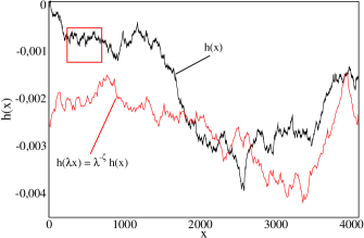
Figure 1: (Color on-line) If a surface of a given linear size $L_{1}$ is with $L_{2}=\lambda L_{1}$ in the horizontal direction, the surface must be scaled with $h(\lambda x)=\lambda^{-\zeta}h(x)$ in the vertical direction to be statistically similar. $\zeta$ is the roughness, or Hurst exponent, measuring the degree of anisotropy. $\zeta=1$ gives self-similar scaling. In this figure the part of the black profile which is inside the square is rescaled with the scaling relation above.

Systems with a common roughness exponent are said to belong to the same universality class, and are therefore controlled by the same fundamental physical law. An early summary of different universality classes and the different surfaces studied can be found in Barabási and Stanley Barabási and Stanley (1995).

The surfaces described above are constructed in different ways. Restricting the discussion to two-dimensional surfaces or profiles we can divide the profiles into three groups. The first group of profiles grow from an initial planar profile or line into a rough profile. Examples from this group of profiles are wetting fronts, deposition fronts and three dimensional fracture surfaces constrained to grow in a plane. The second group of profiles grow at the end points. Examples from this group of profiles are DNA base-pair sequences, any times series and fractures growing in two-dimensional systems. The third group is made by coalescence of micro cracks. Examples from this group of cracks is crack growth by plastic micro void coalescence. The initially flat profiles are often characterized by the Family-Vicsek scaling relation of the profile width $w(L,t)\propto L^{\alpha}f(t/L^{z})$ Family and Vicsek (1985),where $\alpha$ is the roughness exponent measured when the system is saturated and $z=\alpha/\beta$ is the dynamic exponent. $\beta$ is the growth exponent characterizing the growth of the profile width before saturation $w(L,t)\propto t^{\beta}$ The values of the three exponents then give the universality class. Profiles that do not obey Family-Vicsek scaling are said to have anomalous scaling.

The concept of anomalous scaling can not be applied to the second group of profiles as they are only $1+1$ dimensional, while the profiles in the first group are $2+1$ dimensional. The fracture profile in two dimensions are strictly speaking not $1+1$ dimensional since there are two space dimensions and no time dimension. Each single part of the fracture is frozen once it is placed in the system. It is therefore no time evolution of the fracture in $2+1$ dimensions.

The aim of this paper is to give a survey of the different methods used for measuring the roughness exponent and give an estimate of the expected errors and biases. This paper will use some of the methods used by Schmittbuhl et al. in Schmittbuhl et al. (1995), excluding the fractal measurements and the return methods since these methods have already been tested there. We repeat the test done with the local window methods and the power spectrum density analysis. Other methods such as the detrended fluctuation analysis Peng et al. (1994), the averaged wavelet coefficient methodSimonsen et al. (1998) and the height difference distribution are also included. To accurately asses the results from the different methods the methods must be applied to profiles with known roughness exponent. Both the Voss method Voss (1985) and the wavelet method Simonsen and Hansen (2002) for generating profiles have been used and analyzed. We will also study the systematic error introduced by adding a power law noise to the signal, and discuss that both long range correlations in the sign change and a power law noise can give surfaces with roughness exponents. This is motivated by recent results for the central force and fuse model of fracture.Bakke et al. (2007); Bakke and Hansen (2007). Our interest in the phenomena of self-affine surfaces comes from the studies of fracture surfaces both experimental and numerical, and the difficulties we have encountered while measuring the roughness exponent.

The structure of this paper is as follows: In Sec. II the different measurement methods are presented. In Sec.  III we presents the results from the measurements done on the generated profiles. Samples of the power law scaling for each method is presented and compared with the other methods. The results for both the generation methods described in the last paragraph are shown. We find that the power spectrum density analysis and the averaged wavelet coefficient method give the most accurate for roughness exponents in the range $0.1-0.9$. In Sec. IV we study the size dependence on the systematic errors for the different methods. We observe as expected that the errors decreases for larger system sizes, but several of the measuring methods have relatively large systematic error and the size of this error depends on the measured roughness exponent. In Sec. V we show that power law noise might disguise as self-affinity when profiles are analyzed with some methods. We then describe how one can separate the contribution from the power law noise and the sign change correlation to the roughness exponent. And finally in Sec. VI we give a summary and come with some recommendations to researchers studying surface roughness.

II Measurements of the roughness exponent

Until recently one used different methods for measuring the roughness exponent on experimental and numerically made fracture surfaces. On surfaces from experiments one applied local (or intrinsic) methods which use scaling with a (intrinsic) length scale $l$ much smaller than the system size $L$ or spectral methods like the power spectrum density. On the other hand, for surfaces from numerical simulations one applied global (or extrinsic) methods which use scaling with the system size. This was was done by necessity as in experiments it is not easy to make samples of the same material with sizes ranging over several orders of magnitude, or experimental setups that can do measurements over the same orders of magnitude. While for numerical simulations the restriction in computing power made it difficult to create large enough samples to use the local methods. But during the last few years and due to the growth in computing power numerical simulations of fracture have produced large enough samples in such numbers that both the real space and spectral local methods are used in numerical studies of fracture surfaces.

Below we will describe some local and global methods which are used today for measuring the roughness exponent. All the methods we consider in this paper work on profiles. I. e. profiles in two-dimensional planes cut from a surface embedded in three dimensions or a one-dimensional trace or path embedded in two-dimensions.

The local window methods all measure the scaling of a characteristic width as a function of the window size. The width is a measure of how large the fluctuations of the profiles in a window of length $l$ are. We will look at three different methods which use different definitions of the characteristic width: 1. The variable bandwidth method (VB)

$$w_{VB}(l)=(\langle(h(x)-\bar{h})^{2}\rangle_{L})^{1/2}\propto l^{\zeta}\mbox{,}$$ (2)

where $\bar{h}=\langle h(x)\rangle$. 2. The detrended fluctuation analysis (DFA), where the local linear trend in each window is subtracted

$$w_{DFA}(l)=(\langle(h^{\prime}(x)-\bar{h^{\prime}})^{2}\rangle_{L})^{1/2}\propto l^{\zeta}\mbox{.}$$ (3)

3. the maximum - minimum method (MM)

$$w_{MM}(l) = \langle\mbox{max}(h(x),x\in\{x_{o},x_{o}+l\}$$ (4)

$$-\mbox{min}(h(x),x\in\{x_{o},x_{o}+l\}\rangle_{L}\propto l^{\zeta}.$$

$\langle\cdots\rangle_{L}$ means averaging over the system size $L$. Averaging over different samples is implied. The roughness exponent $\zeta$ is then found as the power law scaling with $l$ of the characteristic width.

An alternative measuring method is to look at the second order correlation function

$$C_{2}(r)=\langle(h(x-r)-h(x))^{2}\rangle_{L}^{1/2}\propto r^{\zeta};$$ (5)

The roughness exponent can also be found from the two spectral methods as the scaling of the power spectrum $P(k)$, Falconer (1990) which is the Fourier transform of the correlation function Eq. (5), with the wave number for the power spectrum analysis

$$P(k)\propto k^{-2(\zeta+1)}\mbox{,}$$ (6)

and as the scaling of the averaged wavelets coefficients $W[h](a)$ as a function of the scale variable $a$

$$W[h](a)\propto a^{+\zeta+1/2}.$$ (7)

The global average width method is similar to the intrinsic one, but with the window size $l$ substituted with the system size $L$.

$$W(L)=\langle h(x)-\bar{h}\rangle\propto L^{\zeta}\mbox{,}$$ (8)

Similarly we have the global maximum-minimum method

$$W_{MM}(L) = \langle\mbox{max}(h(x),x\in\{0,L\}$$ (9)

$$-\mbox{min}(h(x),x\in\{0,L\}\rangle\propto L^{\zeta}.$$

The roughness exponent measured by the global methods give the same results as the local methods only of the scaling of $W(L)$ is the same as the scaling of $w(l)$, $l\ll L$. One example of when this is not the case is when the profiles shows anomalous scaling. López and Rodríguez (1996) In this paper we will not consider the global methods.

In two recent papers the question of whether the fracture surfaces measured in experiments are self-affine or multi-affine has been discussed. Bouchbinder et al. (2006); Santucci et al. (2006) In Santucci et al. Santucci et al. (2006) two slightly different methods for measuring the fracture roughness have been discussed. The basis for these methods is to assume that the distribution function $p(\Delta h,l)$, $\Delta h(l)=h(x+l)-h(x)$ is ’Gaussian-like’. The first method was introduced in the studies of directed polymers in random media. Halpin-Healy (1991). The $k$-th moment of $h(x)$. is defined below

$$C_{k}(l)=\langle|h(x+l)-h(x)|^{k}\rangle^{1/k}$$ (10)

To check whether or not the surface have self-affine or multi-affine scaling one calculates the ratio of the $k$-th to the second moment

$$R_{k}(l)=\frac{\langle|h(x+l)-h(x)|^{k}\rangle^{1/k}}{\langle(h(x+l)-h(x))^{2}\rangle^{1/2}}$$ (11)

which for a true Gaussian distribution should reduce to

$$R_{K}^{G}(l)=R_{K}^{G}=\sqrt{2}\left(\Gamma(\frac{\left(\frac{k+1}{2})\right)}{\sqrt{\pi}}\right)^{1/k}.$$ (12)

By plotting $R_{k}/R_{k}^{G}$ one should then get straight lines if the surface is self-affine since $\zeta_{k}=k\zeta$ when the surface is self-affine. If these lines should fall on top of each other, the underlying distribution is also Gaussian. The roughness exponent can be found by finding the slope of $C_{k}/C_{k}^{G}$, where $C_{K}^{G}$ is the $k$-th moment for a true Gaussian distribution, in a double logarithmic plot, which will return the same roughness exponent as $C_{2}(r)$.

The other method is to construct the distributions $p(\Delta h,l)$ of the height difference over distance $l$ and plotting $p(\Delta h,l)\sqrt{2\pi\sigma^{2}}$ versus $(\Delta h)/\sqrt{2\sigma^{2}}$, where $\sigma^{2}$ is the fluctuations of $\Delta h$ over $l$. For Gaussian distributions the plot should be a parabola pointing downward in a semi-logarithmic plot. The roughness exponent can then be found from the power law scaling of slope of the fluctuations in $\Delta h$, $\sigma(l)\propto l^{\zeta}$.

Many of the methods described above involve the scaling of a characteristic width with a window length. At least two mechanisms can lead to the increase in the characteristic width.Falconer (1990) The first one is that there are spatial correlations in the sign change of the steps in the profile, and the second one is a Lévy like jump distribution. To check how these two mechanisms contribute to the measured effective roughness exponent on can do two different modifications to the measured profiles. If one sets the size of each jump equal to unity using

$$h_{0}(x)=\lim_{q\rightarrow 0}\int_{0}^{L}\mbox{sgn}(h(x))|h(x)|^{q}dx\mbox{,}$$ (13)

one will only measure the characteristic width that are caused by the correlations in the sign changes as any information carried by the amplitude will be removed. It has been shown Hansen and Mathiesen (2006) that for $h_{0}(x)$ the roughness exponent is

$$\zeta=\max(\frac{1}{2},\zeta_{h})$$ (14)

where $\zeta_{h}$ is the roughness exponent of $h(x)$. Thus for a roughness exponent less $1/2$ some information in the roughness exponent will be in the jump distribution.

To remove any correlation that might be in the sign changes, but keep the information in the jump distribution one can randomly rearrange the position for each jump. The characteristic width measured on this randomly rearrange profiles $h_{r}(x)$ will now only depend on the jump distribution, and therefore the measured roughness exponent is due to the jumps.

III Accuracy of the measurement methods

In Schmittbuhl et al. Schmittbuhl et al. (1995) the reliability of self-affine measurements is addressed for some of the methods above. We will repeat the measurements for the power spectrum density analysis and local window methods, and compare with the additional methods from Sec. II to check the validity of the roughness exponents we measure from the generated self-affine fracture surfaces.

We base our choice of good measurement methods on two criteria: 1. The fitting of the power law should be good i.e. good linearity in the double logarithmic plots. 2. The systematic error for the method should be small and stable over a range of different roughnesses.

We generate artificial surfaces using two methods. The first method is the Voss method Voss (1985), and the second is the wavelet method Simonsen and Hansen (2002). The profiles are generated by first creating long profiles of a length much larger than the profile sizes we want to study. We then cut out a piece of desired length at a random position from the long profiles. In this study the long profiles had a length of 65536. Before we measure the roughness exponent we remove any linear trend in profiles. The tests are done for $\zeta\in\{0.1,0.9\}$ and system sizes $L\leq 16384$. For each roughness exponent and each system size $100$ samples were generated. Samples of these profiles are shown in Fig. 2. Before one starts to measure the roughness exponent it is from our experience always a good idea to visually inspect the profiles and compare them to self-affine profiles with known roughness exponents.

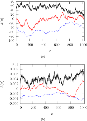
Figure 2: (Color on-line) Sample profiles from the Voss algorithm (a) and the wavelet algorithm (b). The profiles are from top to bottom for roughnesses $0.2$, $0.5$ and $0.8$. To make the scale of the fluctuations the same for samples with different $\zeta$ the samples are rescaled with $W_{\zeta}(L)/W_{0.5}(L)$.

In Figs. 3 to 7 we present the different measurements for $L=512$. This system size is now numerically accessible for many different numerical models of fracture and large enough to give good estimates for the roughness exponent using the local methods. The profiles were made with $\zeta=0.6$ and all straight lines in the figures represents this $\zeta$-value. These plots are from the Voss profiles. From Fig. 3 one see that for the local window methods in Eq. (2) to Eq. (4) the detrended fluctuation analysis gives the best estimate of the roughness exponent. The detrended fluctuation analysis gives a straight line in the double logarithmic plot from $l=16$ to $l=512$ while the variable bandwidth and the Max-Min data are more curved compared to the $\zeta=0.6$ lines.

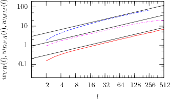
Figure 3: (Color on-line) Measurements of the roughness exponent using intrinsic window methods. From the top: The local MAX-MIN method Eq. (4), the variable bandwidth method Eq. (2) and the detrended fluctuation analysis Eq. 3.

The power spectrum density method in Fig. 4 as well as the averaged wavelet coefficients method in Fig. 5 both give good estimates of the roughness exponent. For $C_{k}/C_{k}^{G}$ we can see in Fig. 6 that the second order correlation function gives an estimate of the roughness exponent comparable which is below the correct value. In addition we see that the collapse of the different moments is showing that the profiles are self-affine, not multi-affine. Fig. 7 shows the scaling of $\sigma(l)$ which give results similar to the second order correlation function.

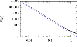
Figure 4: (Color on-line) Measurements of the roughness exponent using the power spectrum density analysis, Eq. 6.

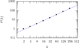
Figure 5: (Color on-line) Measurements of the roughness exponent using the averaged wavelet coefficients method Eq. 7.

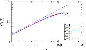
Figure 6: (Color on-line) Measurements of the roughness exponent using second order correlation function Eq. (5).

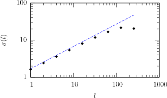
Figure 7: (Color on-line) Measurements of the roughness exponent using the scaling of $\sigma(l)$ for the distribution $p(\Delta H,l)$

When we compared the result for the profiles made with the Voss algorithm in Fig. 8 and the profiles made with the wavelet method in Fig. 9 we notice some differences. Using the power spectrum density analysis and the averaged wavelet coefficients methods the profiles made by both methods we obtain good measurements of the roughness exponent. The results for when using the averaged wavelet coefficient method on the wavelet generated profiles were no surprise as this should a priori give correct results. When one use the detrended fluctuation analysis and the variable bandwidth, the Max-Min and $C_{2}$ methods we see a more pronounced deviation from the true roughness exponent used to create the profiles for the highest $\zeta$ for the wavelet generated profiles.

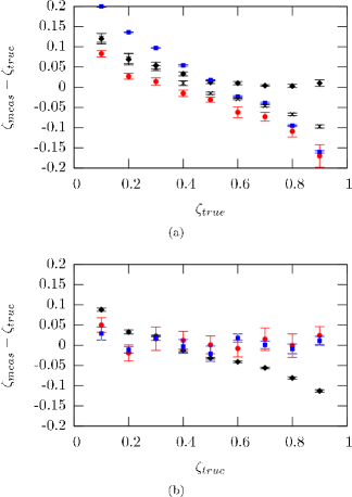
Figure 8: (Color on-line) $\zeta_{measured}-\zeta_{true}$ for profiles generated by the Voss algorithm. a) The detrended fluctuation analysis ($\blacklozenge$), the variable bandwidth ($\bullet$), the Max-Min ($\blacksquare$) and the standard deviation of $\Delta h(l)$ ($+$). b) Second order correlation function ($\blacklozenge$), power spectrum density analysis ($\bullet$) and averaged wavelet coefficients ($\blacksquare$).

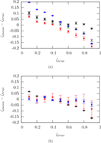
Figure 9: (Color on-line) $\zeta_{measured}-\zeta_{true}$ for profiles generated by the wavelet algorithm. a) The detrended fluctuation analysis ($\blacklozenge$), the variable bandwidth ($\bullet$), the Max-Min ($\blacksquare$) and the standard deviation of $\Delta h(l)$ ($+$). b) Second order correlation function ($\blacklozenge$), power spectrum density analysis ($\bullet$) and averaged wavelet coefficients ($\blacksquare$).

This result suggests that the profiles made by the wavelet method is not as good as the Voss methods for generating self-affine profiles. A test of the self-affinity of the profiles confirms this. In Fig. 10 we clearly see that the wavelet generated profiles have corrections to scaling at small scales. This correction to scaling can also be seen for $p(\Delta h,l)$ in Fig. 11. For the high $\zeta$-values the wavelet generated profiles the tail is broader than a Gaussian distribution. This effect becomes larger for the largest $\zeta$s. The profiles generated by the Voss algorithm is more narrow than the Gaussian distribution, and also for these profiles is the effect greatest for the largest $\zeta$-values. In the rest of this paper we will only consider the profiles made by the Voss method.

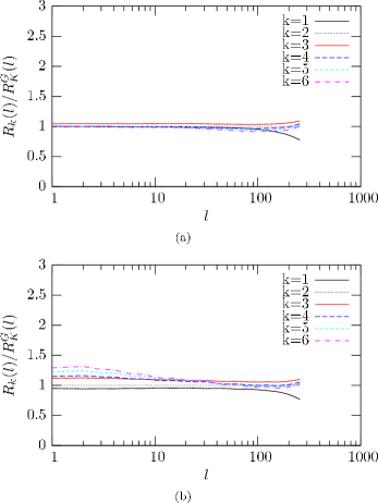
Figure 10: (Color on-line) $R_{k}/R_{k}^{G}$ for profiles of length 512 made by a) the Voss algorithm and b) the wavelet method for $\zeta=0.7$.

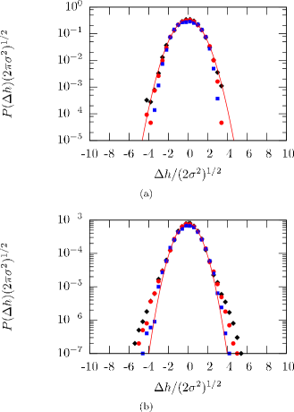
Figure 11: (Color on-line) $p(\Delta h,l)$ for profiles of length $512$ made by a) the Voss algorithm and b) the wavelet method for $\zeta=0.7$ Three different length scales are presented here: $l=64$ ($\blacklozenge$), $l=128$ ($\bullet$) and $l=256$ ($\blacksquare$).

From Figs. 8 and 9 one can see that the power spectrum density analysis and the averaged wavelet coefficients method give the best estimates for the roughness exponent in the range $0.1-0.9$. For these two methods the test measurements done here gave error bars from the power law fits equal or less than $0.03$. The detrended fluctuation analysis gave good estimates above $\zeta=0.5$, and systematically to high estimates for $\zeta<0.5$. The other local methods did only give good estimates around $\zeta=0.5$, and showed an systematic drift towards lower $\zeta$ values for $\zeta>0.5$, and towards higher $\zeta$ values for $\zeta<0.5$. Of the global $W(L)$ gave the most accurate estimates, but gave systematically to high estimates for $\zeta<0.5$.

The results for the roughness exponent were done with the following limits on for the regions where we did a least square fit. For the variable bandwidth method, the Max-Min method and detrended fluctuation analysis the regression was done in the range $l\in[16,L/2]$. For the second order correlation function the regression was done for $l\in[2,L/8]$. For the power spectrum analysis the regression was done for $k\in[0,0.2]$. For the averaged wavelet coefficients method the regression was done for $a\in[8,L/4]$. For the standard deviation of the height-difference the regression was done for $l\in[1,L/16]$.

We conclude this section by checking that the roughness exponent we measure from the profiles generated by the Voss algorithm that the self-affine scaling originates from the long range correlations in the sign changes. From the original profiles $h(x)$ we construct the profile $h_{0}(x)$ where all jumps are on equal size. When $\zeta>0.5$ one sees from Fig. 12 the same general results as presented above for $h(x)$. The power spectrum analysis, the averaged wavelet coefficients method and the detrended fluctuation analysis give the best estimates. However all estimates are from these three methods are now systematically $0.05$ to low compared to the true value. Also the global methods give good estimates, but these are also to low. The other local methods show the same large errors as they did for $h(x)$.

When $\zeta<0.5$ the picture is is not that clear. The results for all the different methods show that they measure values above $\zeta_{h}$, but below $1/2$ showing that not all the self-affine information for $\zeta<0.5$ is in the sign change correlations for the self-affine profiles generated with the Voss algorithm.

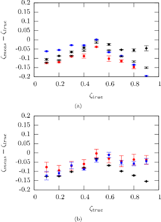
Figure 12: (Color on-line) $\zeta_{measured}-\zeta_{true}$ for $h_{0}(x)$ for profiles generated with the Voss algorithm. $L=512$. a) The detrended fluctuation analysis ($\blacklozenge$), the variable bandwidth ($\bullet$), the Max-Min ($\blacksquare$) and the standard deviation of $\Delta h(l)$ ($+$). b) Second order correlation function ($\blacklozenge$), power spectrum density analysis ($\bullet$) and averaged wavelet coefficients ($\blacksquare$).

IV Size dependence

In the last section we described how the different measurement methods behaved for profiles with $L=512$. In this section we will expand our study by considering how the roughness exponent estimates change with the system size. The accuracy with which one can measure the roughness exponent is dependent of the length of profiles. In Schmittbuhl et al. (1995) Schmittbuhl et al. reported on the size dependence of the error bars for the variable bandwidth method, the MAX-MIN method and the power spectrum analysis. We have performed the measurements of the roughness exponent with the methods described above on samples generated by the Voss algorithm for different system sizes. The results are presented in Fig. 13 to Fig. 21.

As the system size increase the error decreases for the all the measurement methods. But even for large system sizes the different methods measure the $\zeta$ with systematic errors which are dependent on the value of the $\zeta$. These systematic errors are similar to the ones shown in Fig. 8.

The detrended fluctuation analysis, the power spectrum density analysis and the averaged wavelet coefficient method all have systematic errors smaller that $0.05$ for $L\geq 256$ for all values of $\zeta$. The local window methods and the second order correlation function method over-estimate $\zeta$ for $\zeta<0.5$, and under-estimate $\zeta$ for $\zeta\geq 0.5$ as reported in Sec. III.

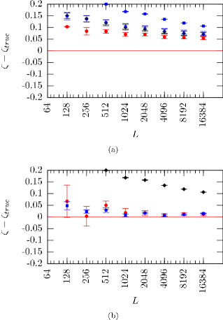
Figure 13: (Color on-line) Systematic errors in roughness exponent measurements versus system size for $\zeta_{true}=0.1$. a) The detrended fluctuation analysis ($\blacklozenge$), the variable bandwidth ($\bullet$), the Max-Min ($\blacksquare$) and the standard deviation of $\Delta h(l)$ ($\times$). b) Second order correlation function ($\blacklozenge$), power spectrum density analysis ($\bullet$) and averaged wavelet coefficients ($\blacksquare$).

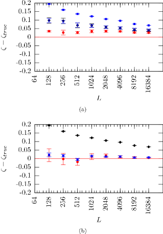
Figure 14: (Color on-line) Systematic errors in roughness exponent measurements versus system size for $\zeta_{true}=0.2$. a) The detrended fluctuation analysis ($\blacklozenge$), the variable bandwidth ($\bullet$), the Max-Min ($\blacksquare$) and the standard deviation of $\Delta h(l)$ ($\times$). b) Second order correlation function ($\blacklozenge$), power spectrum density analysis ($\bullet$) and averaged wavelet coefficients ($\blacksquare$).

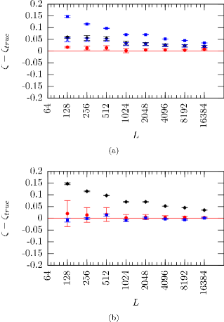
Figure 15: (Color on-line) Systematic errors in roughness exponent measurements versus system size for $\zeta_{true}=0.3$. a) The detrended fluctuation analysis ($\blacklozenge$), the variable bandwidth ($\bullet$), the Max-Min ($\blacksquare$) and the standard deviation of $\Delta h(l)$ ($\times$). b) Second order correlation function ($\blacklozenge$), power spectrum density analysis ($\bullet$) and averaged wavelet coefficients ($\blacksquare$).

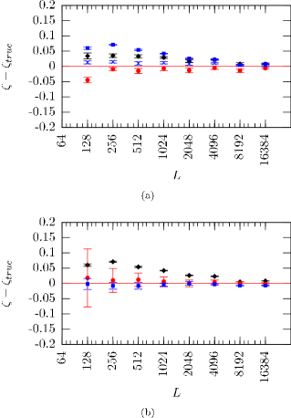
Figure 16: (Color on-line) Systematic errors in roughness exponent measurements versus system size for $\zeta_{true}=0.4$. a) The detrended fluctuation analysis ($\blacklozenge$), the variable bandwidth ($\bullet$), the Max-Min ($\blacksquare$) and the standard deviation of $\Delta h(l)$ ($\times$). b) Second order correlation function ($\blacklozenge$), power spectrum density analysis ($\bullet$) and averaged wavelet coefficients ($\blacksquare$).

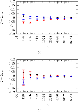
Figure 17: (Color on-line) Systematic errors in roughness exponent measurements versus system size for $\zeta_{true}=0.5$. a) The detrended fluctuation analysis ($\blacklozenge$), the variable bandwidth ($\bullet$), the Max-Min ($\blacksquare$) and the standard deviation of $\Delta h(l)$ ($\times$). b) Second order correlation function ($\blacklozenge$), power spectrum density analysis ($\bullet$) and averaged wavelet coefficients ($\blacksquare$).

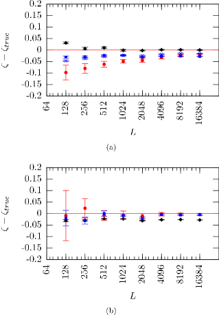
Figure 18: (Color on-line) Systematic errors in roughness exponent measurements versus system size for $\zeta_{true}=0.6$. a) The detrended fluctuation analysis ($\blacklozenge$), the variable bandwidth ($\bullet$), the Max-Min ($\blacksquare$) and the standard deviation of $\Delta h(l)$ ($\times$). b) Second order correlation function ($\blacklozenge$), power spectrum density analysis ($\bullet$) and averaged wavelet coefficients ($\blacksquare$).

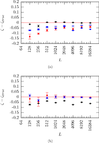
Figure 19: (Color on-line) Systematic errors in roughness exponent measurements versus system size for $\zeta_{true}=0.7$. a) The detrended fluctuation analysis ($\blacklozenge$), the variable bandwidth ($\bullet$), the Max-Min ($\blacksquare$) and the standard deviation of $\Delta h(l)$ ($\times$). b) Second order correlation function ($\blacklozenge$), power spectrum density analysis ($\bullet$) and averaged wavelet coefficients ($\blacksquare$).

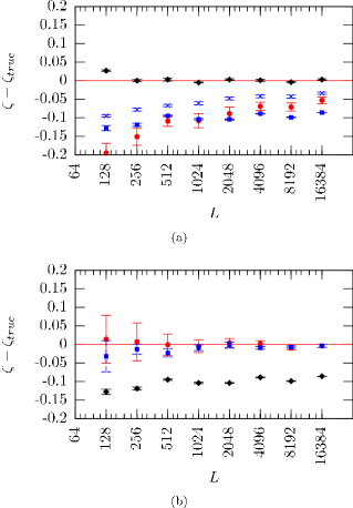
Figure 20: (Color on-line) Systematic errors in roughness exponent measurements versus system size for $\zeta_{true}=0.8$. a) The detrended fluctuation analysis ($\blacklozenge$), the variable bandwidth ($\bullet$), the Max-Min ($\blacksquare$) and the standard deviation of $\Delta h(l)$ ($\times$). b) Second order correlation function ($\blacklozenge$), power spectrum density analysis ($\bullet$) and averaged wavelet coefficients ($\blacksquare$).

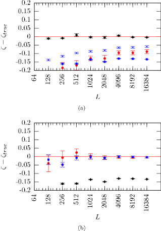
Figure 21: (Color on-line) Systematic errors in roughness exponent measurements versus system size for $\zeta_{true}=0.9$. a) The detrended fluctuation analysis ($\blacklozenge$), the variable bandwidth ($\bullet$), the Max-Min ($\blacksquare$) and the standard deviation of $\Delta h(l)$ ($\times$). b) Second order correlation function ($\blacklozenge$), power spectrum density analysis ($\bullet$) and averaged wavelet coefficients ($\blacksquare$).

V Power law distributed step sizes

We will in this section compare two different sets of profiles which have the same roughness exponent when measured with the detrended fluctuation analysis, but different when measured with the power spectrum density analysis. In Fig. 22 one sample profile from each set of profiles are shown. One profile made with the Voss algorithm with $\zeta_{true}=0.7$, and one profile which is a random walk with Lévy-distributed jumps with $\alpha=1.5$ are shown. As seen in Fig. 22 the main difference between these two profiles are the existence of the large jumps in the second profile. When one use the detrended fluctuation analysis to measure the roughness exponent for these different sets of profiles it gives the same roughness exponent for both sets as shown in Fig. 23. The only difference is that the amplitude of $w_{DFA}(l)$ is larger for the Lévy-flight profiles than for the Voss profiles. If one use the power spectrum analysis, one will measure two different roughness exponents. $\zeta=0.7$ for the profiles made with the Voss algorithm, and $\zeta=0.5$ for the Lévy profiles.

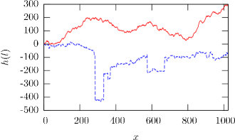
Figure 22: (Color on-line) Two samples profiles of length $1024$, the one with solid lines are made with the Voss algorithm with $\zeta_{true}=0.7$, and the dashed one is a random walk with Lévy-distributed jumps with $\alpha=1.5$

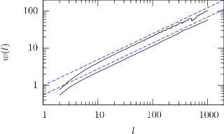
Figure 23: (Color on-line) Roughness exponent measured with detrended fluctuation analysis for a profile made with the Voss algorithm with $\zeta_{true}=0.7$(top) and from a random walk with Lévy-distributed jumps with $\alpha=1.5$(bottom).Both the straight dashed lines in the figure show $\zeta=0.7$. 100 samples of length for each type of profiles were used in the calculations of the roughness exponent.

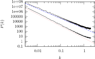
Figure 24: (Color on-line) Roughness exponent measured with PSD for a profile made with the Voss algorithm with $\zeta_{true}=0.7$(bottom) and from a random walk with Lévy-distributed jumps with $\alpha=1.5$(top). The corresponding straight lines are for $\zeta=0.5$ (top) and $\zeta=0.7$ (bottom). 100 samples of length for each type of profiles were used in the calculations of the roughness exponent.

By using the two modified profiles $h_{0}(x)$ and $h_{r}(x)$ described in Sec. II and measuring the roughness exponent on these one can distinguish between the two different sets of profiles. From Table 1 one sees that the power spectrum density analysis do not measure $\zeta\neq 0.5$ for the random walk with Lévy-distributed jumps. Detrended fluctuation analysis will measure $\zeta=0.7$ except when the jumps are all set to the same size. For the profiles generated with the Voss algorithm both the detrended fluctuation analysis and the power spectrum density analysis give $\zeta=0.7$ except for when the long range correlations are destroyed in $h_{r}(x)$. This again show that the roughness exponent for $\zeta\geq 0.5$ for the Voss generated profiles comes from the correlations in the sign change. It also shows that the effective roughness exponent measured with the detrended fluctuation analysis on the Lévy profiles are caused by the power law noise and not the sign change correlation. In addition one notes that different measurement methods give completely different roughness exponents in this case.

Table 1: Table of roughness exponent measured with the detrended fluctuation analysis and the power spectrum analysis on the original profiles ($\zeta$), the modified profiles with equal jump size ($\zeta_{0}$) and the randomly rearranged profiles ($\zeta_{r}$).

Method	DFA			PSD
Profile set	$\zeta$	$\zeta_{0}$	$\zeta_{r}$	$\zeta$	$\zeta_{0}$	$\zeta_{r}$
Voss	0.7	0.7	0.5	0.7	0.7	0.5
Lévy	0.7	0.5	0.7	0.5	0.5	0.5

The power law noise give different corrections to the different measuring methods describe in Sec. II as was shown earlier in this section. To quantify these corrections we have done roughness exponent measurements on random walks on which we impose a power law jump distribution with different exponents. The length of the samples were $1024$ and the number of sample were $1000$. For power laws with exponents in the range $\alpha\in\{0.5,3.0\}$ we observe corrections for the local window methods and the averaged wavelet coefficients method. As seen in Fig. 25 the corrections are less than $0.05$ for $\alpha\geq 2.0$ and increasing for smaller values of $\alpha$.

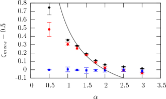
Figure 25: (Color on-line) Roughness measurements on random walks with power law distributed jumps. The detrended fluctuation analysis ($\blacklozenge$), the variable bandwidth method ($\bullet$) and the power spectrum density analysis ($\blacksquare$). The solid line is the roughness exponent for a Lévy-flight, $\zeta_{LF}=1/\alpha$

A Lévy-flight is defined as

$$h(l)=\sum_{i=1}^{l}\Delta h_{i}$$ (15)

where $\Delta h_{i}$ are independent increments following the power law distribution described above. From Bouchaud and Gorges Bouchaud and Gorges (1990) one has that

$$w(l)=\langle|h(l)-\bar{h}(l)|^{2}\rangle\propto l^{1/\alpha},$$ (16)

which gives a roughness exponent $\zeta_{LF}=\alpha^{-1}$. When $\alpha>1.2$ $\zeta$ measured with the local window methods and the averaged wavelet coefficient method follow $\zeta_{LF}$ within $0.05$. For $\alpha<1.2$ $\zeta$ can not keep up with the increasing $\zeta_{LF}$, which also increases beyond 1. This is as expected for the variable bandwidth and the Max-Min methods as they are restricted to measure roughness exponents in the range $\zeta=[0,1]$. The power spectrum analysis and the second order correlation function however measures the correlations in the sign change and will only measure $\zeta=1/2$ for any $\alpha$ value as the jumps are uncorrelated.

As seen above two completely different profiles can with some methods give the same roughness exponent when there is power law distributed noise in the profiles. In addition this power law noise can give multi-affine corrections to the self-affine scaling.

Unfortunately fracture profiles from experiments and simulations often have noise which partly or completely disturb the self-affine property of the profile. This noise can come from the discretization of the data during recording of the profile, the grain or fiber size of the material or from overhangs in the fracture front. For numerical fracture models recent results show that the overhangs in the fracture front have a power law size distribution. Bakke et al. (2007); Bakke and Hansen (2007) In Barabási and Stanley Barabási and Stanley (1995), roughening of a surface with an uncorrelated power law noise is shown to give multi-affinity below a correlation length $l_{X}$ which depends on the strength of the power law noise given by the exponent $\alpha$, i.e. $p(\Delta h)\propto\Delta h^{-\alpha}$, and in Mitchell (2005) Mitchell shows that discontinuities in a self-affine surface give multi-affinity. The random walks with a power law jump distribution a have multi-affine behavior on small scales. The region with corrections to scaling due to multi-affinity changes with $\alpha$ as seen in Fig. 26. Here one sees that the profiles are multi-affine for scales smaller than $20$ for $\alpha=3.0$ and not self-affine at all for $\alpha=1.5$

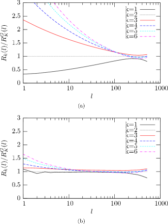
Figure 26: $R_{k}/R_{k}^{G}$ for random walks of length $1024$ with a power law step size distribution with exponent a) $1.5$ and b $3.0$.

VI Summary

For the system size we have studied here the power spectrum analysis and the averaged wavelet coefficient methods gave the best estimates for the roughness exponent over the range of roughness exponents studied here. While the averaged wavelet coefficient method is reported to give more accurate results for a smaller number of samples, Simonsen et al. (1998) this method is prone to systematic errors from power law noise. This also applies to the local window methods. We have also seen that using the different methods might give roughness exponents that differs with a much as $0.1$ with additional errors. In addition several of the methods have systematic errors that varies with the value of the roughness exponent.

As previously stated by Schmittbuhl et al. Schmittbuhl et al. (1995) one should use several different methods for measuring the roughness exponent. Researchers measuring the roughness exponent should also take great care in uncover the noise present in the surfaces that are to be studied. This to make sure that the measuring methods chosen are capable of measuring the roughness exponent properly.

Acknowledgments: We want to thank Ingve Simonsen for enlightening discussions on Lévy-flights.

References

- Bouchaud et al. (1990) E. Bouchaud, G. Lapasset, and J. Planés, Europhys. Lett. 13, 72 (1990).
- Bouchbinder et al. (2006) E. Bouchbinder, I. Procaccia, S. Santucci, and L. Vanel, Phys. Rev. Lett. 96, 055509 (2006).
- Santucci et al. (2006) S. Santucci, K. J. Måløy, A. Delaplace, J. Mathisen, A. Hansen, J. Ø. H. Bakke, J. Schmittbuhl, L. Vanel, and P. Ray (2006), Phys. Rev. E 75, 016104 (2007).
- Mandelbrot et al. (1984) B. B. Mandelbrot, D. E. Passoja, and A. J. Paully, Nature 308, 721 (1984).
- Barabási and Stanley (1995) A. L. Barabási and H. E. Stanley, Fractal Concepts in Surface Growth (Cambridge University Press, 1995).
- Family and Vicsek (1985) F. Family and T. Vicsek, J. Phys. A 18, L75 (1985).
- Schmittbuhl et al. (1995) J. Schmittbuhl, J.-P. Vilotte, and S. Roux, Phys. Rev. E 51, 131 (1995).
- Peng et al. (1994) C.-K. Peng, S. V. Buldyrev, S. Havlin, M. Simons, H. E. Stanley, and A. L. Goldberger, Phys. Rev. E 49, 1685 (1994).
- Simonsen et al. (1998) I. Simonsen, A. Hansen, and O. M. Nes, Phys. Rev. E 58, 2779 (1998).
- Voss (1985) R. F. Voss, Scaling Phenomena in Disorder Systems (Plenu,, 1985).
- Simonsen and Hansen (2002) I. Simonsen and A. Hansen, Phys. Rev. E 65, 037701 (2002).
- Bakke et al. (2007) J. Ø. H. Bakke, T. Ramstad, and A. Hansen (2007), Accepted for publication in Physical Review B.
- Bakke and Hansen (2007) J. Ø. H. Bakke and A. Hansen (2007), in preparation.
- Falconer (1990) K. Falconer, Fractal Geometry: Mathematical Foundations and Applications (John Wiley & Sons, 1990).
- López and Rodríguez (1996) J. M. López and M. A. Rodríguez, Phys. Rev. E 54, R2189 (1996).
- Halpin-Healy (1991) T. Halpin-Healy, Phys. Rev. A 44, R3415 (1991).
- Hansen and Mathiesen (2006) A. Hansen and J. Mathiesen, Survey of scaling surfaces (Springer, 2006), chap. 5.
- Bouchaud and Gorges (1990) J.-P. Bouchaud and A. Gorges, Physics Reports 195, 127 (1990).
- Mitchell (2005) S. J. Mitchell, Phys. Rev. E 72, 065103(R) (2005).