Theory of spin, electronic and transport properties of the lateral triple quantum dot molecule in a magnetic field

Abstract

We present a theory of spin, electronic and transport properties of a few-electron lateral triangular triple quantum dot molecule in a magnetic field. Our theory is based on a generalization of a Hubbard model and the Linear Combination of Harmonic Orbitals combined with Configuration Interaction method (LCHO-CI) for arbitrary magnetic fields. The few-particle spectra obtained as a function of the magnetic field exhibit Aharonov-Bohm oscillations. As a result, by changing the magnetic field it is possible to engineer the degeneracies of single-particle levels, and thus control the total spin of the many-electron system. For the triple dot with two and four electrons we find oscillations of total spin due to the singlet-triplet transitions occurring periodically in the magnetic field. In the three-electron system we find a transition from a magnetically frustrated to the spin-polarized state. We discuss the impact of these phase transitions on the addition spectrum and the spin blockade of the lateral triple quantum dot molecule.

I Introduction

There is currently interest in developing the ability to control and manipulate the total spin of individually localized interacting electrons as a prerequisite for solid-state nanospintronic and quantum information applications.Awschalom et al. (2002); Brum and Hawrylak (1997); Loss and DiVincenzo (1998); DiVincenzo et al. (2000); A.S. Sachrajda and Ciorga (2003) Precise control over the number and spatial location of carriers can be achieved by confining them in lateral gated quantum dot devices, of which the single,Ciorga et al. (2000); Tarucha et al. (1996) double,Holleitner et al. (2002); Pioro-Ladriere et al. (2005); Koppens et al. (2005); Petta et al. (2005); Hatano et al. (2005) and tripleVidan et al. (2004, 2005); Gaudreau et al. (2006); Ihn et al. (2007) quantum dots have already been demonstrated. In particular, Gaudreau et al.Gaudreau et al. (2006); Korkusinski et al. (2007) reported a controlled charging of a lateral triple quantum dot (TQD) molecule with $N=1-6$ electrons, with the ability to control the population of each dot independently. Preliminary experiments on quantum dot molecules in external magnetic field by Gaudreau et al.Gaudreau et al. (2007) and by Ihn et al.Ihn et al. (2007) showed signatures of Aharonov-Bohm (AB) oscillations, indicating coherent coupling between the constituent dots. In this work we present a theory of the magnetic field effect on the electronic, spin, and transport properties of an isolated triple quantum dot molecule with controlled number of electrons $N=1-6$.

Previous theoretical descriptions of isolated lateral multi-quantum dot devices in a magnetic field focused on quantum dot molecules with one electron per dot using Hubbard, exact numerical diagonalization, and spin Heisenberg model.Scarola and DasSarma (2005); Scarola et al. (2004) They showed magnetic field induced corrections to the Heisenberg model due to chiral spin interactions. Furthermore, for three dots in a triangular structure, one electron each, they established magnetic field-induced transitions from a lowest-energy spin doublet with total spin $S=1/2$ (Ref. Hawrylak and Korkusinski, 2005) to $S=3/2$ spin polarized state.Scarola et al. (2004); Scarola and DasSarma (2005) Spin transitions in isolated lateral multi-quantum dot devices with large electrons numbers have also been studied using spin density functional theory by Stopa et al.Stopa et al. (2006) There has also been significant interest in triple quantum dots in triangular configuration connected to the leads. Using the Hubbard model the effects of the magnetic field on the conductance through an empty and singly occupied triple dot were studied, with focus on the interplay between the Kondo physics, symmetries, and the AB oscillations.Kuzmenko et al. (2002, 2006); K.Kikoin and Avishai ; Jiang and Sun (2007); Emary

The aim of this work is to study the magnetic field dependence of the electronic properties of the lowest electronic shell of a triangular triple quantum dot molecule filled with $N=1-6$ electrons, extending in this way our previous workKorkusinski et al. (2007) to finite magnetic fields. This is accomplished by both the analysis of the Hubbard model and by the development of a new computational tool. The new microscopic tool combines (i) a calculation of single particle states as a linear combination of harmonic orbitals (LCHO) localized on each dot, with a proper gauge transformation allowing for convergent results as a function of the ratio of the magnetic length to the inter-dot separation, with (ii) configuration-interaction approach (CI) to the many-electron problem. These techniques have allowed us to analyze the spin and electronic properties as a function of the magnetic field and the number $N$ of confined electrons ($N=1$ up to $6$). We derive the magnetic-field evolution of the one-electron spectrum and show the existence of degeneracies at multiples of half flux quanta threading the area of the TQD, in agreement with Ref. Kuzmenko et al., 2002. The magnetic field-engineered degeneracies of single-particle levels, combined with electron-electron exchange and correlations, allow for the control of the total spin of the many-electron system. For example, we show total spin oscillations due to the singlet-triplet transitions occurring periodically in the magnetic field for two and four electron molecules. In the three-electron system we find the magnetic field-induced transition from a magnetically frustrated to the spin-polarized state, in agreement with Refs. Scarola et al., 2004; Scarola and DasSarma, 2005. We discuss the impact of these spin transitions on the addition spectrum as measured using charge spectroscopy, and predict the appearance of spin blockade in the transport through TQD molecule.

The paper is organized as follows. In Sec. II we present details of the Hubbard and LCHO-CI approaches. In Sec. III we calculate the electronic structure of the triple dot filled with $N=1$ to $6$ electrons as a function of the magnetic field. The discussion of the charging diagram and addition amplitudes is presented in Sec. IV. The paper is summarized in Sec. V.

II The model

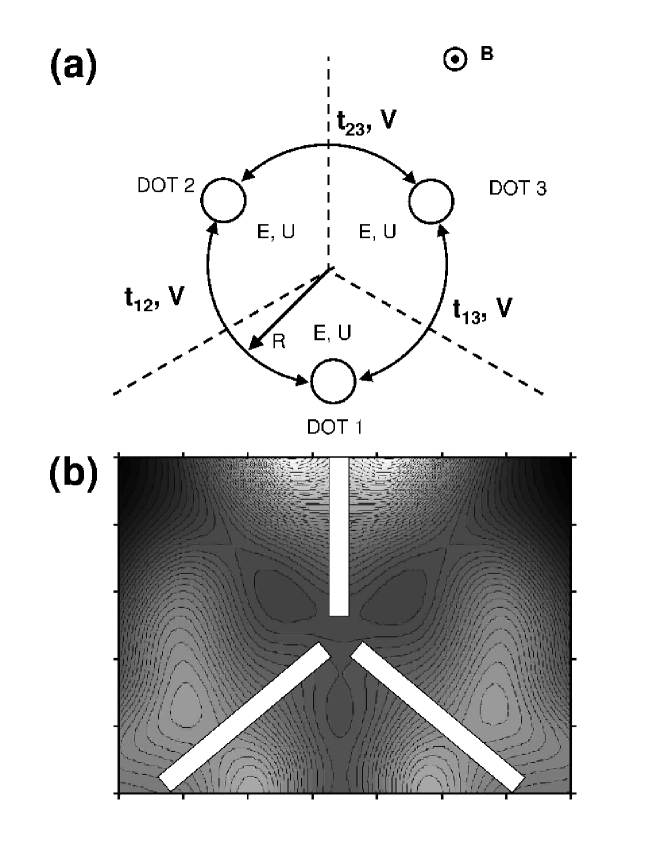
Figure 1: (a) Schematic image of the triple-dot molecule. Symbols denote the Hubbard parameters for the system on resonance. The magnetic field is perpendicular to the plane of the molecule. (b) Contour plot of the potential created in the lateral triple-dot device by a typical layout of the metallic gates. White zones show schematically the gates controlling the barriers between dots.

A schematic picture of the TQD studied in this work is shown in Fig. 1(a). This system is an approximation of the lateral gated TQD device, in which the three potential minima are created electrostatically by metallic gates. Such device has been studied theoretically in Refs. Hawrylak and Korkusinski, 2005; Korkusinski et al., 2007 and is related to the system demonstrated experimentally by Gaudreau et al.Gaudreau et al. (2006) Figure 1(b) shows the TQD electrostatic potential generated by a model arrangement of gates enclosing the area of the device (not shown) together with additional gates (shown as white regions) used to establish the potential barriers between the dots. By selective tuning of the voltages it is possible to bring the three dots into resonance, i.e., match the energies of the lowest single-particle orbital of each potential minimum. The resulting TQD molecule can be then filled controllably with $N$ electrons, starting at $N=1$, in the presence of a magnetic field ${\bf B}=[0,0,B]$ applied in the direction perpendicular to the plane of the system.

II.1 Hubbard model

We have shown previouslyKorkusinski et al. (2007) that the electronic properties of the molecule with few confined electrons ($N=1$ to $6$) can be understood in the frame of the Hubbard model. Assuming one orbital with energy $E_{i,\sigma}$ in each dot, the Hubbard Hamiltonian can be written as

$$\hat{H}_{H}=\sum_{\sigma,i=1}^{3}E_{i,\sigma}c_{i\sigma}^{\dagger}c_{i\sigma}+\sum\limits_{\sigma,i,j=1,i\neq j}^{3}t_{ij}(B)c_{i\sigma}^{\dagger}c_{j\sigma}+U\sum\limits_{i=1}^{3}n_{i\downarrow}n_{i\uparrow}+{1\over{2}}V\sum\limits_{i,j=1,i\neq j}^{3}\varrho_{i}\varrho_{j},$$ (1)

where the operators $c_{i\sigma}$ ($c_{i\sigma}^{\dagger}$) annihilate (create) an electron with spin $\sigma=\pm 1/2$ in dot $i$. Further, $n_{i\sigma}=c_{i\sigma}^{\dagger}c_{i\sigma}$ and $\varrho_{i}=n_{i\downarrow}+n_{i\uparrow}$ are, respectively, the spin and charge density on the $i$th dot. In Eq. (1), $t_{ij}(B)$ is the matrix element describing tunneling between dots $i$ and $j$, $U$ is the onsite Coulomb repulsion, and $V$ is the direct repulsion of electrons occupying neighboring dots.

In the Hamiltonian (1) the magnetic field $B$ is accounted for in two terms. First, it introduces the Zeeman splitting in the onsite energies $E_{i,\sigma}=E_{i}+g^{*}\mu B\sigma$, with $g^{*}$ being the effective Landé factor and $\mu_{B}$ being the Bohr magneton. Second, it renormalizes the single-particle tunneling elements $t_{ij}$ by Peierls phase factors,Peierls (1933); Luttinger (1951) such that $t_{ij}(B)=t_{ij}e^{2\pi i\phi_{ij}}$. For the three quantum dots located in the corners of an equilateral triangle we have $\phi_{12}=\phi_{23}=\phi_{31}=-\phi/3$. Here, $\phi=3\sqrt{3}eBR^{2}/8\pi\hbar c$ is the number of magnetic flux quanta threading the system, with $e$ being the electron charge, $c$ - the speed of light, $\hbar$ - the Planck’s constant, and $R$ - the distance from the center of the triangle to each dot, identified in Fig. 1(a).

With one spin-degenerate orbital per dot we can fill the TQD with up to $N=6$ electrons. To find the eigenenergies and eigenstates of $N$ electrons we use the configuration interaction approach (CI), in which we create all possible configurations of $N$ electrons on the localized orbitals, write the Hamiltonian $\hat{H}_{H}$ in a matrix form in this basis, and diagonalize the resulting matrix numerically.Korkusinski et al. (2007)

II.2 LCHO-CI method

We compare the results of the Hubbard model with a microscopic approach to the calculation of the electronic properties of a TQD starting from a confining potential, which we outline in this section. We start by expressing all energies in units of the effective Rydberg ${\cal R}=m_{e}^{*}e^{4}/2\varepsilon^{2}\hbar^{2}$, and lengths in the effective Bohr radius, $a_{B}=\varepsilon\hbar^{2}/m_{e}^{*}e^{2}$, where $m^{*}$ is the electron effective mass and $\varepsilon$ is the dielectric constant of the material. With GaAs parameters, $m_{e}^{*}=0.067$ $m_{0}$ and $\varepsilon=12.4$, we have ${\cal R}=5.93$ meV and $a_{B}=9.79$ nm.

A single electron in the TQD in the presence of an external perpendicular magnetic field is described by the Hamiltonian

$$\hat{H}_{0}=\left(-i\nabla+\mathbf{A}(\mathbf{r})\right)^{2}+\sum_{i=1}^{3}V_{i}(\mathbf{r})+V_{B}(\mathbf{r})$$ (2)

where $\mathbf{A}(\mathbf{r})$ is the effective vector potential, $V_{i}(\mathbf{r})$ is the confining potential of the $i$-th dot, and $V_{B}(\mathbf{r})$ is the potential due to the additional gates, which control the potential barriers between dots.

We choose the vector potential in the symmetric gauge $\mathbf{A}(\mathbf{r})=\Omega_{c}/4(-y\hat{\mathbf{x}}+x\hat{\mathbf{y}})$ centered at the geometric center of the triangle of the dots.Scarola et al. (2004) Here the cyclotron energy $\Omega_{c}=\hbar\omega_{c}/{\cal R}$ with $\omega_{c}=eB/m_{e}^{*}c$. The confining potential of each dot is approximated by a Gaussian $V_{i}(\mathbf{r})=-V_{i,0}\exp\left[-\left({\mathbf{r}-\mathbf{r}_{i}\over d_{i}}\right)^{2}\right]$. Further we separate the Gaussian potential into the harmonic and anharmonic parts,

$$V_{i}(\mathbf{r})=-V_{i,0}+\frac{\Omega_{i,0}^{2}}{4}\left({\mathbf{r}-\mathbf{r}_{i}\over d_{i}}\right)^{2}+\delta V_{i},=V^{HO}_{i}+\delta V_{i}$$ (3)

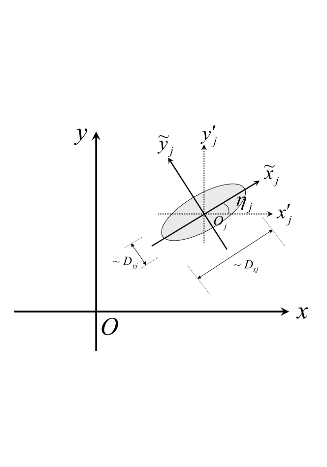
Figure 2: Schematic picture of the potential created by one of the Gaussian barrier centered at $(x_{Bj},y_{Bj})$ and the relation between the original variables $(x,y)$ and the system $(\tilde{x}_{j},\tilde{y}_{j})$.

where $\Omega_{i,0}=2\sqrt{V_{i,0}}/d_{i}$ is the effective characteristic energy of the harmonic confinement. In order to tune the height of the tunneling barrier between dots independently of the confining potential, we introduce Gaussian barrier potentials located between each pair of dots.Abolfath and Hawrylak (2007) In the device depicted in Fig. 1(b) these potentials are generated by the gates shown as white regions. The coordinate system used to define the Gaussian barriers is summarized in Fig. 2. Here we assume that the narrow gate is oriented along the axis $\tilde{x}$, which means that the geometry in Fig. 2 applies specifically to the lower left-hand gate of Fig. 1(b). The Gaussian barrier can now be defined as

$$V_{B}(\mathbf{r})=\sum_{j=1}^{3}V_{B}^{(j)}(\mathbf{r})=V_{B0}^{(j)}\mathrm{exp}\left(-\frac{\tilde{x}_{j}^{2}}{D_{xj}^{2}}-\frac{\tilde{y}_{j}^{2}}{D_{yj}^{2}}\right),$$ (4)

with the global and local coordinate systems related by

$$\tilde{x}_{j} = (x-x_{Bj})\cos\eta_{j}+(y-y_{Bj})\sin\eta_{j}$$

$$\tilde{y}_{j} = -(x-x_{Bj})\sin\eta_{j}+(y-y_{Bj})\cos\eta_{j}.$$ (5)

If we choose both the global gauge $\mathbf{A}(\mathbf{r})$ and a computational basis centered at the origin of a TQD,Scarola et al. (2004); Scarola and DasSarma (2005) we find a very poor convergence of results as a function of the size of single-particle basis, especially for large interdot distances, when each dot should essentially be considered separately, with its own vector potential.Abolfath and Hawrylak (2007) To remedy this, we divide the system into three regions, whose boundaries are marked in Fig. 1(a) by dashed lines, and in each region define the vector potential in the form

$$\mathbf{A}_{i}=\frac{\Omega_{c}}{4}\left[-(y-y_{i})\hat{\mathbf{x}}+(x-x_{i})\hat{\mathbf{y}}\right],$$ (6)

i.e., centered in the potential minimum of the respective dot.

We solve for the eigenenergies and eigenvectors of the Hamiltonian (2) in the basis composed of harmonic oscillator states (HO) of each dot in the magnetic field

$$\langle\mathbf{r}|inm\rangle=\phi_{inm}(\mathbf{r})=\mathrm{exp}\left[-i\frac{\Omega_{c}}{4}(-y_{i}x+x_{i}y)\right]\phi^{(i)}_{nm}(\mathbf{r}-\mathbf{r}_{i}),$$ (7)

where $\phi^{(i)}_{nm}(\mathbf{r}-\mathbf{r}_{i})$ are the HO orbitals of $i$th dot, satisfying the Schrödinger equation

$$\left[\left(-i\nabla+\mathbf{A}_{i}(\mathbf{r})\right)^{2}+V^{HO}_{i}\right]\phi^{(i)}_{nm}(\mathbf{r}-\mathbf{r}_{i})=\varepsilon_{inm}^{HO}\phi^{(i)}_{nm}(\mathbf{r}-\mathbf{r}_{i}).$$ (8)

The energy associated with the HO state $\phi^{(i)}_{nm}$,

$$\varepsilon_{inm}^{HO}=-V_{i,0}+\Omega_{i,+}\left(n+\frac{1}{2}\right)+\Omega_{i,-}\left(m+\frac{1}{2}\right),$$ (9)

is defined in terms of energies $\Omega_{i,\pm}=\Omega_{i,h}\pm\Omega_{c}/2$, with the hybrid energy $\Omega_{i,h}=\sqrt{\Omega_{i,0}^{2}+\Omega_{c}^{2}/4}$. The eigenfunctions of Eq. (8) are the Fock-Darwin (FD) orbitals, whose explicit form as a function of $z=x+iy$ and $\bar{z}=x-iy$ is

$$\phi^{(i)}_{nm}(\mathbf{r})=\frac{(-1)^{n_{2}}}{\sqrt{2\pi l_{i,h}^{2}}}\sqrt{\frac{n_{2}!}{n_{1}!}}\,\mathrm{L}_{n_{2}}^{n_{1}-n_{2}}\left(\frac{z\bar{z}}{2l_{i,h}^{2}}\right)e^{-\frac{z\bar{z}}{4l_{i,h}^{2}}}\left\{\begin{array}[]{l}\left(\bar{z}/\sqrt{2}l_{i,h}\right)^{m-n}\quad\mathrm{for}\quad m\geq n\\ \left(z/\sqrt{2}l_{i,h}\right)^{n-m}\quad\mathrm{for}\quad n\geq m\end{array}\right.$$ (10)

Here $n_{1}=\mathrm{max}(n,m)$, $n_{2}=\mathrm{min}(n,m)$ and the hybrid length $l_{i,h}=\sqrt{1/\Omega_{i,h}}$. Further, $\mathrm{L}_{n}^{k}$ is the generalized Laguerre polynomial defined as

$$\mathrm{L}^{k}_{n}(x)=\sum_{l=0}^{n}\frac{(-1)^{l}(n+k)!}{(n-l)!(k+l)!l!}x^{l}~{},\quad\mathrm{for}\quad k>-1~{}.$$ (11)

The phase factor $e^{-\frac{i\Omega_{c}}{4}(-y_{i}x+x_{i}y)}$ of the basis function $\phi_{inm}$ in Eq. (7) is due to the gauge transformation $\mathbf{A}_{i}\Rightarrow\mathbf{A}$. This additional phase factor depends on the magnetic field and the distance of dot $i$ from the origin, and leads to the flux-dependent factor renormalizing the tunneling matrix elements in the Hubbard model.

Now we can represent the single-electron eigenvalue problem of the TQD in matrix form in a restricted Hilbert space formed by $n_{0}$ FD orbitals from each dot, with dimension $N_{orb}=3n_{0}$, as:

$$\mathbf{H}_{0}\mathbf{a}^{(n)}=\varepsilon_{n}\mathbf{S}\mathbf{a}^{(n)}$$ (12)

where $\mathbf{H}_{0}$ is the Hamiltonian matrix for $\hat{H}_{0}$ in Eq. (2) and $\mathbf{S}$ is the overlap matrix due to the non-orthogonality of the basis and $\mathbf{a}^{(n)}$ is an eigenvector corresponding to the eigenvalue $\varepsilon_{n}$. The eigenstates are given by

$$\psi_{n}(\mathbf{r})=\sum_{k=1}^{N_{orb}}a^{(n)}_{k}\phi_{k}(\mathbf{r})$$ (13)

where the composite index $k=\{inm\}$. The Hamiltonian and overlap matrix elements can be obtained efficiently if we expand the FD orbitals as linear combinations of the zero-field HO orbitals $\phi^{(0)}_{n_{x},n_{y}}(\mathbf{r})$ with characteristic, magnetic-field dependent energy $\Omega_{h}$.

$$\phi_{nm}(\mathbf{r})=\sum_{s=0}^{n+m}A_{s}^{nm}\phi^{(0)}_{n+m-s,s}(\mathbf{r}),$$ (14)

where

$$A_{s}^{nm}=\sqrt{\frac{n!m!(n+m-s)!s!}{2^{n}2^{m}}}(-i)^{s}\sum_{k=\mathrm{max}(0,s-m)}^{\mathrm{min}(s,n)}\frac{(-1)^{k}}{k!(n-k)!(s-k)!(m-s+k)!}.$$ (15)

Then the integration needed to obtain the Hamiltonian and overlap matrix elements can be separated into $x$- and $y$-dependent parts and each integral can be carried out analytically. For the barrier potential $V_{B}(\mathbf{r})$ such a separation is complicated by the appearance of an $xy$ term in the exponent. This term can be eliminated by a transformation to the local coordinate system defined in Eq.(5), after which the integrals can be carried out analytically.

The generalized eigenvalue problem formulated in Eq.(12) can be cast into a standard eigenvalue problem

$$\mathbf{H}^{\prime}\mathbf{b}^{(n)}=\varepsilon_{n}\mathbf{b}^{(n)},$$ (16)

where $\mathbf{H}^{\prime}=(\sqrt{\mathbf{S}})^{-1}\mathbf{H}_{0}(\sqrt{\mathbf{S}})^{-1}$ and $\mathbf{b}^{(n)}=\sqrt{\mathbf{S}}\mathbf{a}^{(n)}$. The matrix $\sqrt{\mathbf{S}}$ is found by solving the eigenvalue problem $\mathbf{S}\mathbf{V}_{S}=\mathbf{V}_{S}\mathbf{E}_{S}$. Here $\mathbf{V}_{S}$ is the matrix of eigenvectors and $\mathbf{E}_{S}$ is the diagonal matrix with eigenvalues. Then $\sqrt{\mathbf{S}}$ is obtained by $\sqrt{\mathbf{S}}=\mathbf{V}_{S}^{{\dagger}}\mathbf{E}_{S}^{1/2}\mathbf{V_{S}}$. The off-diagonal elements of the effective Hamiltonian $\mathbf{H}^{\prime}$ correspond to the tunneling elements in the Hubbard model. To see how the gauge transformation automatically takes care of the phase change of the tunneling elements let us consider a resonant TQD system where all three confining potentials are identical. Since we will consider only $s$ orbitals from each dot (i.e., $n=m=0$), we shall use the simplified notation $|i00\rangle\equiv|i\rangle$. Then the off-diagonal matrix element of the Hamiltonian $\mathbf{H}_{0}$ are

$$\langle i|\hat{H}_{0}|j\rangle=\Omega_{0}\langle i|j\rangle+\langle i|-\frac{\Omega_{0}^{2}}{4}(\mathbf{r}-\mathbf{r}_{j})^{2}|j\rangle+\langle i|\sum_{k=1}^{3}V_{k}(\mathbf{r})|j\rangle~{}.$$ (17)

The overlap matrix element takes the form

$$\langle i|j\rangle=\exp\left[\frac{i\Omega_{c}}{4}\hat{\mathbf{z}}\cdot(\mathbf{r}_{i}\times\mathbf{r}_{j})-\frac{(\mathbf{r}_{i}-\mathbf{r}_{j})^{2}}{8}\left(\frac{1}{l_{h}^{2}}+\frac{l_{h}^{2}\Omega_{c}^{2}}{4}\right)\right]$$ (18)

and the second term in Eq. (17) is

$$\langle i|-\frac{\Omega_{0}}{4}(\mathbf{r}-\mathbf{r}_{j})^{2}|j\rangle=-\frac{\Omega_{0}^{2}l_{h}^{2}}{4}\langle i|j\rangle\left[2+\frac{(\mathbf{r}_{i}-\mathbf{r}_{j})^{2}}{4}\left(\frac{1}{l_{h}^{2}}-\frac{l_{h}^{2}\Omega_{c}^{2}}{4}\right)\right].$$ (19)

If we neglect the three-center integrals $\langle i|V_{k}(\mathbf{r})|j\rangle$ for $k\neq i,j$, the last term in Eq. (17) is obtained in the form

$$\langle i|V_{i}(\mathbf{r})+V_{j}(\mathbf{r})|j\rangle=\frac{-2V_{0}d^{2}}{2l_{h}^{2}+d^{2}}\exp\left[\frac{i\Omega_{c}}{4}\hat{\mathbf{z}}\cdot(\mathbf{r}_{i}\times\mathbf{r}_{j})-\frac{(\mathbf{r}_{i}-\mathbf{r}_{j})^{2}}{2(2l_{h}^{2}+d^{2})}\left(1+\frac{d^{2}}{4l_{h}^{2}}+\frac{\Omega_{c}^{2}l_{h}^{2}d^{2}}{16}\right)\right].$$ (20)

The common overall phase $\frac{\Omega_{c}}{4}\hat{\mathbf{z}}\cdot(\mathbf{r}_{i}\times\mathbf{r}_{j})$ is proportional to the magnetic field and the area of the parallelogram formed by the vectors $\mathbf{r}_{i}$ and $\mathbf{r}_{j}$. Now Eq. (17) becomes

$$\langle i|\hat{H}_{0}|j\rangle=-A_{ij}\exp\left[\frac{i\Omega_{c}}{4}\hat{\mathbf{z}}\cdot(\mathbf{r}_{i}\times\mathbf{r}_{j})\right],$$ (21)

where the amplitude $A_{ij}$ has complicated dependence on the magnetic field but is generally positive and decreases exponentially as the magnetic field increases. This exponential decrease is due to the suppression of the overlap of orbitals from different dots, resulting from the decrease of the effective radius of the wave function with the increasing magnetic field. The off-diagonal element of the effective Hamiltonian $\mathbf{H}^{\prime}$ differs from that in Eq. (17) due to the existence of the overlap matrix $\mathbf{S}$, but the behavior of the phase and the amplitude is the same. Thus the tunneling parameter in the Hubbard model in the presence of magnetic field acquires a field-dependent phase proportional to the flux, and amplitude which decays exponentially with the flux.

The eigenstates of the above single-electron problem are linear combinations of the harmonic oscillator orbitals (LCHO). We use these LCHO extended molecular orbitals to solve the many-electron problem of the TQD system. The Hamiltonian of this system is

$$\hat{H}=\sum_{i\sigma}(\varepsilon_{i}+\varepsilon^{Z}_{\sigma})c_{i\sigma}^{{\dagger}}c_{i\sigma}+\frac{1}{2}\sum_{ijkl\sigma\sigma^{\prime}}\langle ij|v_{c}|kl\rangle c_{i\sigma}^{{\dagger}}c_{j\sigma^{\prime}}^{{\dagger}}c_{k\sigma^{\prime}}c_{l\sigma}$$ (22)

where $i$, $j$, $k$, $l$ enumerate the LCHO orbitals and $\sigma$,$\sigma^{\prime}$ are spin indices. The operators $c^{{\dagger}}_{i\sigma}$ $(c_{i\sigma})$ create (annihilate) an electron on the spin-orbital $(i,\sigma)$, while $\varepsilon^{Z}_{\sigma}=g^{*}m_{e}^{*}\Omega_{c}\sigma/2m_{0}$ is the Zeeman energy. In the following discussions, the Zeeman energy is accounted for only in the sections corresponding to three electrons and the addition spectra, where it is responsible for the transition between spin polarized and spin unpolarized ground state. In order to make the transition more clear in the corresponding figures, we have chosen a model value of $g^{*}=-0.02$ instead of the usual value corresponding to GaAs ($g^{*}=-0.44$).

The second term of the above Hamiltonian is scaled by Coulomb interaction matrix elements

$$\langle ij|v_{c}|kl\rangle=\int d\mathbf{r}\int d\mathbf{r}^{\prime}\psi_{i}^{*}(\mathbf{r})\psi_{j}^{*}(\mathbf{r}^{\prime})\frac{2}{|\mathbf{r}-\mathbf{r}^{\prime}|}\psi_{k}(\mathbf{r}^{\prime})\psi_{l}(\mathbf{r}).$$ (23)

Using the Fourier transformation of the Coulomb interaction,

$$\langle ij|v_{c}|kl\rangle = \frac{1}{\pi}\int_{0}^{\infty}dq\int_{0}^{2\pi}d\theta_{q}\int d\mathbf{r}\psi_{i}^{*}(\mathbf{r})e^{i\mathbf{q}\cdot\mathbf{r}}\psi_{l}(\mathbf{r})\int d\mathbf{r}^{\prime}\psi_{j}^{*}(\mathbf{r}^{\prime})e^{-i\mathbf{q}\cdot\mathbf{r}^{\prime}}\psi_{k}(\mathbf{r}^{\prime})$$ (24)

$$= \frac{1}{\pi}\int_{0}^{\infty}dq\int_{0}^{2\pi}d\theta_{q}\langle i|e^{i\mathbf{q}\cdot\mathbf{r}}|l\rangle\langle j|e^{-i\mathbf{q}\cdot\mathbf{r}}|k\rangle~{}.$$

The matrix elements of the plane wave $\langle i|e^{i\mathbf{q}\cdot\mathbf{r}}|j\rangle$ are evaluated analytically using the expansions (13 - 14) of the LCHO orbitals in terms of the zero-field HO orbitals. The $q$ and $\theta_{q}$ integrations are then carried out numerically. The Coulomb interaction matrix elements can be used to extract the interaction parameters in the Hubbard model.

While the LCHO-CI approach is general, we will illustrate it on the TQD molecule with identical quantum dots. For a given number of electrons, we consider all possible configurations of electrons in the LCHO orbitals, calculate the Hamiltonian matrix in this configuration basis and diagonalize this matrix numerically to find the eigenstates and eigenenergies of the interacting many-electron TQD. In this paper, we consider single-particle basis formed by $s$ orbitals from each dot and filling of the lowest electronic shell with $N=1-6$ electrons.

III Magnetic field behavior of the lowest electronic shell

III.1 Magnetic field dependence of single-electron spectrum

Let us start our analysis by discussing the single-particle spectrum of the triple dot molecule as a function of the magnetic field. In the basis of orbitals $\{|1\rangle,|2\rangle,|3\rangle\}$ localized on the respective dots, the Hubbard Hamiltonian for a single electron in the TQD on resonance takes a matrix form

$$\hat{H}_{T}=\left[\begin{array}[]{ccc}E&te^{-2\pi i\phi/3}&te^{2\pi i\phi/3}\\ te^{2\pi i\phi/3}&E&te^{-2\pi i\phi/3}\\ te^{-2\pi i\phi/3}&te^{2\pi i\phi/3}&E\\ \end{array}\right].$$ (28)

The one-electron Hamiltonian can be diagonalized by performing the Fourier transform of the localized basis $|j\rangle$ into a plane wave basis $|K\rangle$ as $|K\rangle=\sum\limits_{j=1}^{3}{e^{iK(j-1)}|j\rangle}$ (Ref. Hawrylak, 1993). The new basis consists of three states, with $K_{1}=0$, $K_{2}=2\pi/3$, and $K_{3}=-2\pi/3$, given by:

$$\left\{\begin{array}[]{ll}|{K_{1}}\rangle=\frac{1}{\sqrt{3}}\left(|1\rangle+|2\rangle+|3\rangle\right)\\ |{K_{2}}\rangle=\frac{1}{\sqrt{3}}\left(|1\rangle+e^{i2\pi/3}|2\rangle+e^{i4\pi/3}|3\rangle\right)\\ |{K_{3}}\rangle=\frac{1}{\sqrt{3}}\left(|1\rangle+e^{-i2\pi/3}|2\rangle+e^{-i4\pi/3}|3\rangle\right).\end{array}\right.$$ (32)

The corresponding eigenenergies are, respectively: $E_{1}=E-2|t|\cos\left(2\pi\phi/3\right)$, $E_{2}=E-2|t|\cos\left[2\pi(\phi+1)/3\right]$, and $E_{3}=E-2|t|\cos\left[2\pi(\phi-1)/3\right]$. At zero magnetic field the three eigenstates form a spectrum with a non-degenerate, standing wave (zero effective angular momentum) $K=0$ ground state, and two degenerate excited states with $K=\pm 2\pi/3$ (effective angular momentum $\pm 1$, respectively).

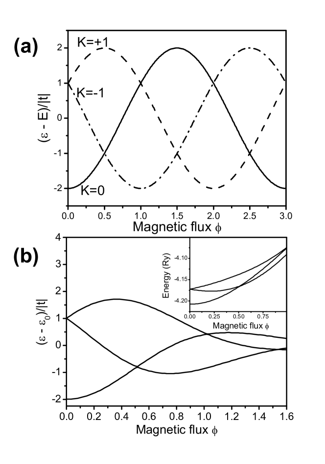
Figure 3: Single-particle energies of the triple dot molecule as a function of the number of magnetic flux quanta calculated within the Hubbard model (a), and with the LCHO approximation (b). In figure (b) the inset corresponds to the actual spectrum while in the main panel the diamagnetic shift has been removed to facilitate the comparison with results from Hubbard model.

In Fig. 3(a) we show these energies as a function of the flux $\phi$, with different lines corresponding to each effective angular momentum. The calculations were performed for model parameters $E=0$ and $t=-0.0118{\cal R}$, and in the absence of the Zeeman energy. We find that the one-electron energy spectrum is composed of three levels, whose energies undergo Aharonov-Bohm oscillations with period $\Delta\phi=3$ flux quanta and amplitude $2|t|$ around the single-dot energy $E$. At $\phi=(2n+1)/2$ with $n=0,1,\dots$ we find a degenerate ground state and a nondegenerate excited state of the system. On the other hand, for $\phi=n$ the degeneracy is inverted, i.e., the ground state is nondegenerate while the excited state is doubly degenerate. The levels correspond to different quantum numbers, and hence cross without interaction, leading to degeneracies.

We tested the behavior of the energy spectrum of the Hubbard model against the microscopic LCHO approach. We assume the depth of the Gaussian potentials $V_{0}=5.864$ ${\cal R}$, their characteristic width $d=2.324$ $a_{B}$, and the distance between dot centers $|\mathbf{r}_{i}-\mathbf{r}_{j}|=4.85$ $a_{B}$ based on fitting to the electrostatic confinement produced by a model lateral gated quantum dot device.Korkusinski et al. (2007) As discussed in the previous section, the flux-dependent phase factor is due to the gauge transformation in LCHO approach. In the inset of Fig. 3(b) we show the single-particle energies as a function of the magnetic flux calculated with the LCHO method with only one HO orbital per dot. The resulting spectrum does exhibit the periodic degeneracies of levels. It differs, however, from that in Fig. 3(a) in two aspects. First, as a function of the magnetic field all energies undergo a diamagnetic shift towards higher energies. This shift is, in most part, due to the behavior of single-dot energies, which in the LCHO approach are $\varepsilon_{i00}^{HO}=\Omega_{h}$, and therefore increase with the magnetic field. In the Hubbard model, on the other hand, we have assumed these energies to be constant, irrespective of the number of flux quanta. In the main panel of Fig. 3(b) we have redrawn the LCHO spectrum with the diamagnetic shift removed by subtracting the reference energy

$$E_{0}=\langle i00|\left[\left(-i\nabla+\mathbf{A}_{i}(\mathbf{r})\right)^{2}+\sum_{j=1}^{3}V_{j}(\mathbf{r})\right]|i00\rangle.$$ (33)

The renormalized spectrum can be directly compared with the energy spectrum of the Hubbard model. Both spectra oscillate with increasing magnetic field. The second difference between the two spectra involves the amplitude of oscillation, which remains constant in the Hubbard approach, but decreases in the LCHO treatment. This feature can be understood in terms of decrease of the magnitude of the effective tunneling parameter $|t|$ with increasing magnetic field. This can be overcome by reducing the height of tunneling barriers between dots using additional gates as discussed in Section II.

From Fig. 3 it is apparent that by adjusting the magnetic field and barrier height we can engineer the degeneracies of the single-particle states. This property of the triple dot molecule is of key importance when the system is being filled with electrons.

III.2 Two electrons

Let us start with $N=2$ electrons confined in the triple dot molecule. In order to simplify the notation, in the following sections, unless the opposite is explicitly stated, we shall denote the complex and magnetic field-dependent hopping parameter $t_{ij}(\phi)$ by $t_{ij}$.

We can classify the two-electron states into singlets and triplets according to their total spin. Let us start with the triplet subspace, with both electrons spin-down. The basis consists of three singly-occupied localized configurations: $|T_{1}\rangle=c^{\dagger}_{2\downarrow}c^{\dagger}_{1\downarrow}|0\rangle$, $|T_{2}\rangle=c^{\dagger}_{1\downarrow}c^{\dagger}_{3\downarrow}|0\rangle$, $|T_{3}\rangle=c^{\dagger}_{3\downarrow}c^{\dagger}_{2\downarrow}|0\rangle$. Each configuration has the same energy $2E+V$, and each pair of configurations is coupled via the single-particle tunneling elements only. Therefore, the Hubbard Hamiltonian written in this basis is identical to the single electron Hamiltonian, Eq. (28), except that all off-diagonal tunneling elements acquire a negative phase. As a result, the triplet eigenvectors $|\bar{T}_{1}\rangle$, $|\bar{T}_{2}\rangle$, $|\bar{T}_{3}\rangle$ can be expressed as Fourier transforms of the basis states $|T_{j}\rangle$ in the same way the single-particle molecular orbitals are expressed in terms of localized orbitals $|j\rangle$, shown in Eq. (32). The two electrons either move clockwise, counterclockwise, or stand still. The three eigenenergies corresponding to these eigenvectors are, respectively, $E_{T}^{1}=2E+V+2|t|\cos\left({2\pi}\phi/3\right)$, $E_{T}^{2}=2E+V+2|t|\cos\left[{2\pi}(\phi+1)/3\right]$, and $E_{T}^{3}=2E+V+2|t|\cos\left[{2\pi}(\phi-1)/3\right]$. Note the difference in sign of $t$ in the eigenvalues with respect to the single electron case. As a result, at zero magnetic field we obtain the doubly degenerate lowest-energy state $E_{T}=2E+V-|t|$, and a non-degenerate excited state with energy $E_{T}=2E+V+2|t|$, As the magnetic field increases, the triplet energies oscillate with the period of $3$ flux quanta.

Let us now move on to the singlet subspace. The singly-occupied singlet configurations $|S_{1}\rangle$, $|S_{2}\rangle$, and $|S_{3}\rangle$ are obtained from the triplet configurations $|T_{1}\rangle$, $|T_{2}\rangle$, and $|T_{3}\rangle$ by flipping the spin of one electron and properly antisymmetrizing the configurations. For example, the configuration $|S_{1}\rangle={1\over\sqrt{2}}\left(c^{\dagger}_{2\downarrow}c^{\dagger}_{1\uparrow}+c^{\dagger}_{1\downarrow}c^{\dagger}_{2\uparrow}\right)|0\rangle$. In the same way, $|S_{2}\rangle={1\over\sqrt{2}}\left(c^{\dagger}_{3\downarrow}c^{\dagger}_{1\uparrow}+c^{\dagger}_{1\downarrow}c^{\dagger}_{3\uparrow}\right)|0\rangle$ and $|S_{3}\rangle={1\over\sqrt{2}}\left(c^{\dagger}_{3\downarrow}c^{\dagger}_{2\uparrow}+c^{\dagger}_{2\downarrow}c^{\dagger}_{3\uparrow}\right)|0\rangle$. In addition to the singly-occupied configurations there are also three doubly-occupied configurations $|S_{4}\rangle$, $|S_{5}\rangle$, and $|S_{6}\rangle$, such that, e.g., $|S_{4}\rangle=c^{\dagger}_{1\downarrow}c^{\dagger}_{1\uparrow}|0\rangle$. The singly-occupied configurations are characterized by energies $2E+V$, and, just as the triplets, they are coupled by tunneling matrix elements. Unlike in the triplet case, however, these off-diagonal elements do not acquire the negative sign. On the other hand, the energies of all doubly-occupied configurations are $2E+U$, i.e., contain the element describing the Coulomb onsite repulsion, making these energies larger than those of the singly-occupied configurations. The Hubbard Hamiltonian does not mix the configurations $|S_{4}\rangle$, $|S_{5}\rangle$, and $|S_{6}\rangle$ with each other, but does mix the singly and doubly occupied subspaces. Here again it is convenient to Fourier transform the singlet basis set into the form $\{|\bar{S_{1}}\rangle,|\bar{S_{2}}\rangle,|\bar{S_{3}}\rangle,|S_{4}\rangle,|S_{5}\rangle,|S_{6}\rangle\}$. In this basis the full singlet Hamiltonian can be written as two $3\times 3$ block diagonal matrix coupled through terms that account for the interactions between singly and doubly occupied configurations:

$$\hat{H}_{S}=\left[\begin{array}[]{cc}\hat{I}{\bf D}_{1}&\hat{C}\\ \hat{C}^{\dagger}&\hat{I}{\bf D}_{2}\end{array}\right],$$ (36)

where $\hat{I}$ is the $3\times 3$ identity matrix, the vector ${\bf D}_{1}^{T}=\left[2E+V-2|t|\cos\left(2\pi\phi/3\right),2E+V-2|t|\cos\left(2\pi(\phi+1)/3\right),2E+V-2|t|\cos\left(2\pi(\phi-1)/3\right)\right]$, and the vector ${\bf D}_{2}^{T}=\left[2E+U,2E+U,2E+U\right]$. The coupling matrix $\hat{C}$ is

$$\hat{C}=-{\sqrt{8\over 3}}|t|\left[\begin{array}[]{ccc}\cos\left(\frac{2\pi\phi}{3}\right)&e^{i2\pi\phi/3}&e^{-i2\pi\phi/3}\\ {1\over 2}e^{-i2\pi\phi/3}\left(1+e^{i2\pi\left(2\phi-1\right)/3}\right)&e^{i2\pi\phi/3}\left(1+e^{-4\pi i/3}\right)&e^{-i2\pi(\phi+1)/3}\left(1+e^{-2\pi i/3}\right)\\ {1\over 2}e^{-i2\pi\phi/3}\left(1+e^{i2\pi(2\phi+1)/3}\right)&e^{i2\pi\phi/3}\left(1+e^{4\pi i/3}\right)&e^{-i2\pi(\phi-1)/3}\left(1+e^{2\pi i/3}\right)\\ \end{array}\right].$$ (40)

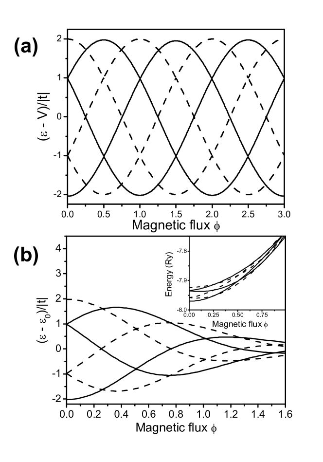
Figure 4: (a) Energy spectrum of the TQD with $N=2$ as a function of the number of magnetic flux quanta calculated within the Hubbard model. Solid lines correspond to the triplet levels, while dashed lines correspond to the singlets. (b) The same energy spectrum calculated with the LCHO-CI approximation after removing the diamagnetic shift. Inset corresponds to the actual spectrum with diamagnetic shift.

In Fig. 4(a) we have plotted the low-energy spectrum for the TQD with 2 electrons, assuming the Hubbard parameters $V=0.42$ ${\cal R}$ and $U=2.56$ ${\cal R}$ (Ref. Korkusinski et al., 2007). The three dashed lines correspond to the eigenvalues of the triplet Hamiltonian while the three solid lines are eigenvalues of the singlet Hamiltonian. For the $6\times 6$ singlet Hamiltonian, there is an additional three-fold degenerate and non-oscillating eigenvalue at higher energy, originating from the doubly-occupied configurations (not shown in the figure). The main result, apparent in Fig. 4(a), is the existence of transitions between the spin singlet and triplet, occurring periodically as a function of the magnetic flux. In the region between $\phi=0$ and $\phi=1$ the ground state is a singlet for $\phi<1/4$ and $\phi>3/4$, and triplet for $1/4<3\phi/4$. This alignment of phases repeats for each subsequent flux quantum.

Upon the inclusion of Zeeman energy we find that the intervals of stability of the singlet phase decrease in each subsequent period. The spin oscillations are eventually suppressed leading to a continuous triplet ground state at sufficiently high magnetic fields.

The existence of spin oscillations is confirmed by results of the LCHO-CI calculation presented in Fig. 4(b). The inset of Fig. 4(b) shows that the diamagnetic shift together with the decrease of tunneling between dots makes it difficult to distinguish more than one oscillation. But after removing the diamagnetic shift by subtracting the reference energy $\varepsilon_{0}$, defined by the ground state energy of the two-electron system without tunneling, the resulting energy spectrum [main panel in Fig. 4(b)] agrees well with the Hubbard model except for the exponential decay of the amplitude of energy oscillations.

III.3 Three electrons

The three electron case at zero magnetic field has been analyzed in detail in Ref. Korkusinski et al., 2007. Following that scheme, we start our treatment with the completely spin-polarized system, i.e., one with total spin $S=3/2$. In this case we can distribute the electrons on the three dots in only one way: one electron on each site with parallel spin, which gives a spin-polarized state $|a_{3/2}\rangle=c^{\dagger}_{3\downarrow}c^{\dagger}_{2\downarrow}c^{\dagger}_{1\downarrow}|0\rangle$. This is an eigenstate of our system with energy $E_{3/2}=3E+3V$. Let us now flip the spin of one of the electrons. This electron can be placed on any orbital, and with each specific placement the remaining two spin-down electrons can be distributed in three ways. Altogether we can generate nine different configurations. Three of these configurations involve single occupancy of the orbitals. They can be written as $|a\rangle=c^{\dagger}_{3\downarrow}c^{\dagger}_{2\downarrow}c^{\dagger}_{1\uparrow}|0\rangle$, $|b\rangle=c^{\dagger}_{1\downarrow}c^{\dagger}_{3\downarrow}c^{\dagger}_{2\uparrow}|0\rangle$, and $|c\rangle=c^{\dagger}_{2\downarrow}c^{\dagger}_{1\downarrow}c^{\dagger}_{3\uparrow}|0\rangle$. The remaining six configurations with double occupancy are $|d\rangle=c^{\dagger}_{2\downarrow}c^{\dagger}_{1\downarrow}c^{\dagger}_{1\uparrow}|0\rangle$, $|e\rangle=c^{\dagger}_{3\downarrow}c^{\dagger}_{1\downarrow}c^{\dagger}_{1\uparrow}|0\rangle$, $|f\rangle=c^{\dagger}_{3\downarrow}c^{\dagger}_{2\downarrow}c^{\dagger}_{2\uparrow}|0\rangle$, $|g\rangle=c^{\dagger}_{1\downarrow}c^{\dagger}_{2\downarrow}c^{\dagger}_{2\uparrow}|0\rangle$, $|h\rangle=c^{\dagger}_{1\downarrow}c^{\dagger}_{3\downarrow}c^{\dagger}_{3\uparrow}|0\rangle$, $|j\rangle=c^{\dagger}_{2\downarrow}c^{\dagger}_{3\downarrow}c^{\dagger}_{3\uparrow}|0\rangle$. All these configurations are characterized by the same projection of total spin, $S_{z}=-1/2$. Moreover, the doubly-occupied configurations are also the eigenstates of total spin, with $S=1/2$, while the total spin of the singly-occupied configurations is not defined. In the basis of the nine configurations we construct the Hamiltonian matrix by dividing the $9$ configurations into three groups, each containing one of the singly-occupied configurations $|a\rangle$, $|b\rangle$, and $|c\rangle$, respectively. By labeling each group with the index of the spin-up electron, the Hamiltonian takes the form of a $3\times 3$ matrix:

$$\hat{H}_{1/2}=\left[\begin{array}[]{ccc}\hat{H}_{1}&\hat{T}_{12}&\hat{T}_{31}^{\dagger}\\ \hat{T}_{12}^{\dagger}&\hat{H}_{2}&\hat{T}_{23}\\ \hat{T}_{31}&\hat{T}_{23}^{\dagger}&\hat{H}_{3}\\ \end{array}\right].$$ (41)

The diagonal matrix, e.g.,

$$\hat{H}_{1}=\left[\begin{array}[]{ccc}3E+2V+U&t_{23}&-t_{13}\\ t_{23}^{*}&3E+2V+U&t_{12}\\ -t_{13}^{*}&t_{12}^{*}&3E+3V\\ \end{array}\right]$$

describes the interaction of three configurations which contain spin-up electron on site 1, i.e., two doubly-occupied configurations $|d\rangle$ and $|e\rangle$, and a singly-occupied configuration $|a\rangle$. The remaining matrices corresponding to spin-up electrons localized on sites 2 and 3 can be constructed in a similar fashion. The interaction between them is given in terms of effective and magnetic field dependent hopping matrix

$$\hat{T}_{ij}=\left[\begin{array}[]{ccc}0&-t_{ij}&0\\ 0&0&-t_{ij}\\ +t_{ij}&0&0\\ \end{array}\right].$$

Upon diagonalization of the Hamiltonian (41) we obtain nine levels, of which one corresponds to the total spin $S=3/2$, and eight - to the total spin $S=1/2$. The energy of the high-spin state is the same as that of the configuration $|a_{3/2}\rangle$ discussed above, except for the Zeeman contribution, which is different due to the different spin projection $S_{z}$ of the two configurations.

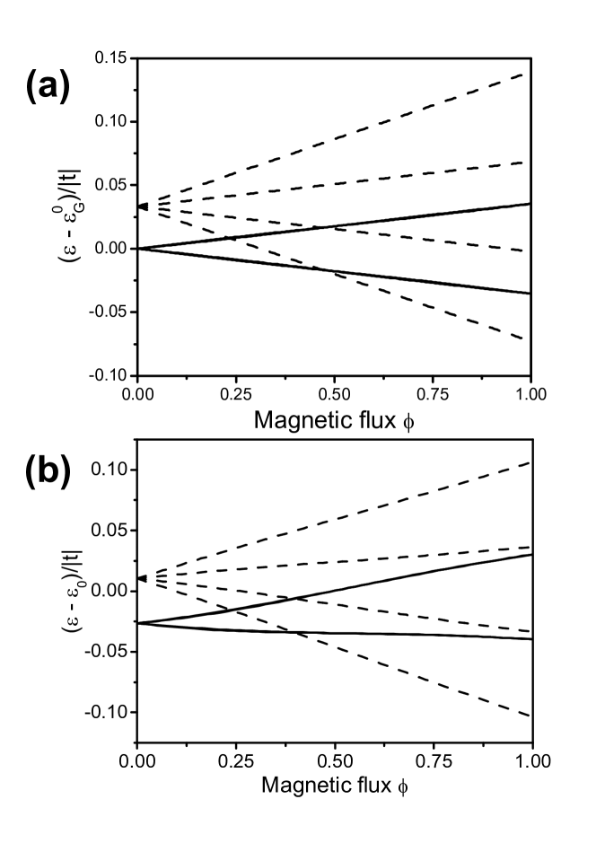
Figure 5: (a) Energy spectrum of the TQD with three electrons versus the dimensionless flux $\phi$ including the Zeeman term. All energies are measured from the ground state energy at $\phi=0$. (b) The same spectrum calculated using the LCHO-CI technique without diamagnetic shift.

Let us now discuss the energy spectrum of the system at zero magnetic field. In Ref. Korkusinski et al., 2007 we have shown that this spectrum is composed of two segments. In the low-energy region we find two $S=1/2$, $S_{z}=-1/2$ states, which form a degenerate pair for the TQD on resonance. At the energy equal to $3J/2$, where $J$ is the exchange energy, we find one $S=3/2$, $S_{z}=-1/2$ state. These three levels are built out of singly-occupied configurations. The high-energy part of the spectrum consists of three pairs of states, composed of doubly-occupied configurations. The two parts of the spectrum are separated by an energy gap proportional to the onsite Coulomb element $U$. In the following we shall focus on the low-energy segment of the spectrum only, shown in Fig. 5(a).

Before we discuss the three-electron spectrum at finite magnetic field, we first account for the correct degeneracy of the energy levels by including states with all possible orientations of the total spin $S_{z}$. In this case we have two pairs of states with low spin: one pair with $S_{z}=+1/2$, and another with $S_{z}=-1/2$. These two pairs form a degenerate quadruplet at $\phi=0$. The high-spin state, on the other hand, is a manifold of four states, with $S_{z}=\pm 3/2$ and $S_{z}=\pm 1/2$. Let us now consider the spectrum at finite magnetic fields accounting for the Zeeman energy. The quadruply degenerate low-spin state splits into two branches separated by the Zeeman energy, see Fig. 5(a),reflecting the different orientations of $S_{z}$. Further, the energies of the states composing each pair oscillate with the magnetic field, and cross each other at $\phi=n\pi/2$, $n=0,1,\dots$ (not seen on this scale). These oscillations have a period $\Delta\phi=1$, different from the period of three flux quanta present for one and two electrons. The amplitude is also a non-trivial function of the hopping parameters $t$, being more than two orders of magnitude smaller than $|t|$. As for the high-spin state, its four-fold degeneracy is lifted by the Zeeman energy, but the constituent levels do not exhibit any oscillations. With increasing magnetic field the $S=3/2,S_{z}=3/2$ spin-polarized state lowers its energy with respect to the ground $S=1/2,S_{z}=1/2$ state, and at a critical value of the magnetic field becomes the ground state. The critical magnetic field $B_{c}$ is given by the condition $g^{*}\mu B_{c}=3J/2$, under which the Zeeman energy equals the exchange energy. The results of the Hubbard calculations are in agreement with the three-electron energy spectra calculated within the LCHO-CI approach, shown in Fig. 5(b). Note that a similar analysis was reported in Ref. Scarola and DasSarma, 2005 for the TQD composed of shallower, parabolic dots with larger interdot tunneling. These calculations revealed an additional total spin oscillation between the $S=1/2$ and $S=3/2$ phases, which occurs for the same $S_{z}$ component. We were able to reproduce this oscillation within the LCHO-CI approach using shallower dots, but not within the Hubbard model. This is because the spin oscillation is due to the magnetically-induced reduction of the interdot tunneling element. However, the importance of these oscillations is minor due to the dominant role of the Zeeman energy. As discussed above, the Zeeman energy leads to the onset of a spin polarized phase at a sufficiently high magnetic field, which suppresses any spin oscillations.

III.4 Four electrons

The four-electron configurations correspond to two holes, created when two electrons are removed from the filled-shell configuration. With two holes we can form only the spin singlet and triplet configurations of the system.

Let us focus on the triplets first. They involve one electron spin-up occupying the first, second, or third dot in the presence of an inert core of three spin-down electrons. If we denote the operator creating a hole on dot $i$ with spin $\sigma$ by $h_{i\sigma}^{\dagger}$, we can write the three basis configurations in this subspace in the form $|T^{(H)}_{1}\rangle=h^{\dagger}_{1\downarrow}h^{\dagger}_{2\downarrow}|N_{e}=6\rangle=c^{\dagger}_{3\uparrow}c^{\dagger}_{3\downarrow}c^{\dagger}_{2\downarrow}c^{\dagger}_{1\downarrow}|0\rangle$, $|T^{(H)}_{2}\rangle=h^{\dagger}_{3\downarrow}h^{\dagger}_{1\downarrow}|N_{e}=6\rangle$ and $|T^{(H)}_{3}\rangle=h^{\dagger}_{3\downarrow}h^{\dagger}_{2\downarrow}|N_{e}=6\rangle$. The two-hole triplet Hamiltonian is given by

$$\hat{H}_{T}=\left[\begin{array}[]{ccc}4E+U+5V&t_{23}&t_{13}\\ t_{23}^{*}&4E+U+5V&t_{12}\\ t_{13}^{*}&t_{12}^{*}&4E+U+5V\\ \end{array}\right].$$ (42)

Note that the above Hamiltonian differs from that describing the two-electron triplet subspace in that the off-diagonal tunneling matrix elements do not acquire the additional negative phase.

Let us move on to the two-hole singlet configurations. The singly-occupied states involve the two holes occupying two different dots, while the doubly-occupied states hold both holes on the same dot. This situation is analogous to the two-electron case described earlier, and the two-hole singlet Hamiltonian written in the appropriately rotated basis is analogous to that shown in Eq. (36). The only difference is that the diagonal vectors ${\bf D}_{1}$ and ${\bf D}_{2}$ will contain two-hole, instead of two-electron energies: $4E+U+5V$ instead of $2E+V$ for singly-occupied configurations, and $4E+2U+4V$ instead of $2E+U$ for doubly-occupied configurations. Also, the factors $|t|$ in ${\bf D}_{1}$ acquire the opposite sign, while this additional phase does not appear in the coupling matrix $\hat{C}$ for the two-hole case.

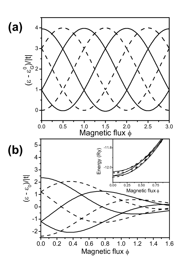
Figure 6: (a) Energy spectrum of the TQD with four electrons versus the dimensionless flux $\phi$ in the absence of Zeeman energy. Triplet levels plotted with dashed lines while singlets are indicated with solid lines. (b) The four-electron spectrum obtained using the LCHO-CI technique with (inset) and without (main panel) diamagnetic shift.

In Ref. Korkusinski et al., 2007 we have diagonalized the singlet and triplet Hamiltonians at zero magnetic field. We found that in this case the total spin of the two-hole ground state depended on the interplay of Hubbard parameters. For a typical case of $2|t|<U-V$ the ground state is a spin triplet. Clearly, the appearance of the finite magnetic moment of the ground state is made possible by the degeneracy of the single-particle excited state at zero magnetic field. As we increase the field this degeneracy is removed, so we may expect a transition to a spin singlet. The periodic reappearance of the degeneracy should lead to spin oscillations. This is indeed what we observe in the energy spectrum, whose low-energy segment is plotted in Fig. 6(a) as a function of the number of magnetic flux quanta. Again, singlet eigenvalues have been plotted with solid lines and dashed lines for the triplets. As for the case of $N=2$, transitions between triplet and singlet ground state appear as we increase the magnetic flux, except that the alignment of phases seen for $N=2$ electrons is inverted. Furthermore, as in the case of two electrons, the introduction of the Zeeman term will favor the spin alignment of the triplet configuration, suppressing the triplet-singlet transitions at high magnetic field. These predictions of the Hubbard model are confirmed by the LCHO-CI calculation, whose results are presented in Fig. 6(b). Again, the original spectrum is shown in the inset, while the main panel shows the energies without the diamagnetic shift.

III.5 Five electrons

Five electrons correspond to a single hole. The single-hole Hamiltonian can be obtained from the single-electron Hamiltonian by appropriately modifying the diagonal terms and setting $t_{ij}\leftrightarrow-t_{ij}$ (Ref. Korkusinski et al., 2007). For the triangular triple dot on resonance this symmetry is reflected in the energy spectrum of the hole as shown in Fig.5(a). For the one-hole problem at zero magnetic field, the opposite sign of the off-diagonal element leads to a doubly-degenerate hole ground state. This behavior is confirmed in the LCHO-CI calculations, whose results are shown in Fig. 5(b).

IV Charging diagram of the resonant triple dot

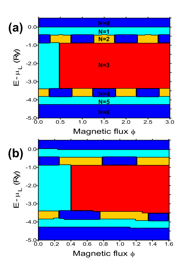
Figure 8: (Color online) (a) Charging diagram for the TQD versus the number of magnetic flux quanta $\phi$ calculated in the Hubbard model. Colors indicate the total spin of the ground state: $S=0$ (blue), $S=1/2$ (cyan), $S=1$ (yellow), and $S=3/2$ (red). (b) The diagram obtained using the LCHO-CI method.

We can now construct the charging diagram of the triple dot molecule as a function of the magnetic field. For any number of electrons $N$ (1 to 6) and any quantum dot energy $E$, we obtain the ground-state energy $E_{GS}(N)$ and the corresponding total spin by diagonalizing the Hubbard Hamiltonian. We use these energies to calculate the chemical potential of the triple quantum dot molecule $\mu(N)=E_{GS}(N+1)-E_{GS}(N)$. When $\mu(N)$ equals the chemical potential $\mu_{L}$ of the leads, the $N+1$st electron is added to the $N$-electron quantum-dot molecule. This establishes the total number of electrons $N$ in the quantum dot molecule and their total spin as a function of quantum-dot energy $E$ relative to the chemical potential of the leads $\mu_{L}$. In the case of LCHO-CI approach, the relevant quantum dot energy is the single-particle reference energy $E$. Changes in electron numbers can be detected by Coulomb blockade (CB), spin blockade, or charging spectroscopies.Pioro-Ladriere et al. (2005); Gaudreau et al. (2006) The calculated stability diagram, with Hubbard parameters used in the previous section and taking into account the contribution of the Zeeman term, is shown in Fig. 8(a), while Fig. 8(b) shows the stability diagram computed using the LCHO-CI approach. Note that in this figure the oscillations of the stability lines corresponding to the condition $\mu(N)-\mu_{L}=0$ are not visible due to the energy scale. As explained in the previous sections, the differences among both addition spectra are due to the diamagnetic shift and the suppression of the inter-dot tunneling. These effects appear naturally in the LCHO-CI approach but are not taken into account in the Hubbard model.

Let us explain the addition spectrum as we change the single-dot energy $E$ of each dot with respect to the chemical potential of the leads $\mu_{L}=0$. From the condition $\mu_{L}=E-2|t|$, the energy $E_{GS}(1)$ corresponding to the addition of the first electron can be approximated by $E(1)\approx 2|t|$. At this energy the first Coulomb blockade peak of the triple quantum dot molecule should be observed. Similar arguments based on the results of the previous section can be applied to find the CB peaks corresponding to the addition of the remaining electrons. Note that the prominent energy gap that appears for the addition of the fourth electron on the TQD is due to the large on-site Coulomb repulsion $U$. The ground state of the three-electron TQD corresponds to one electron occupying each dot, and therefore the addition of a new electron will increase the energy of the system by order of $U$. This term does not appear in any other addition processes, in which only the interdot Coulomb element $V$ is relevant.

The spin oscillations in the system with two and four electrons, as well as the spin transition in the three electron system, lead to a strong modulation of the current through the TQD. An schematic representation of the amplitude of Coulomb blockade peaks as a function of the magnetic flux is given in Fig. 9, for different numbers of electrons confined in the triple dot. Here we assume that the leads are spin-unpolarized, and the transport involves only the lowest-energy level of the molecule. The vertical arrow shows the transition in the three electron system from $S=1/2$ to $S=3/2$ state. When the two electrons are in a spin triplet with $S=1$, adding an electron can create a spin polarized final $S=3/2$ three electron droplet, and the current is high. However, if the two-electron system is in a singlet $S=0$ state, the final $S=3/2$ state cannot be reached by adding a single electron, and the current is spin blockaded. Hence quenching of the tunneling current in the two-electron droplet is a signature of a spin-polarized three-electron state and a spin-singlet two-electron state. Adding a fourth electron to a three-electron droplet is equivalent to adding a hole to a two-hole droplet. Hence the oscillation in CB peak amplitude, but shifted in phase since the holes start as triplets and electrons start as singlets.

V Conclusions

In conclusion, we have studied the effect of the magnetic field on the electronic properties of a triple triangular quantum dot molecule. Exact results for few-electron spectra in a magnetic field where obtained for identical dots in the Hubbard model. Aharonov-Bohm oscillations of a single electron, singlet-triplet spin oscillations for pairs of electrons and pairs of holes, as well as a transition from the frustrated magnetic state to spin polarized state for a half-filled lowest electronic shell are predicted. The impact of spin transitions on the stability diagram and modulation of the current through the TQD molecule with increasing magnetic flux are discussed. The results of the Hubbard model are supported by a microscopic calculation using a general LCHO-CI approach extended to finite magnetic fields.

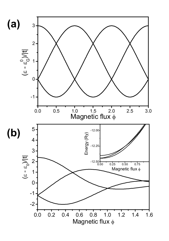
Figure 7: (a) Energy spectrum of the TQD with five electrons versus the dimensionless flux $\phi$, plotted with the zero-field ground-state energy treated as reference. (b) The five-electron spectrum obtained using the LCHO-CI method with (inset) and without (main panel) diamagnetic shift.

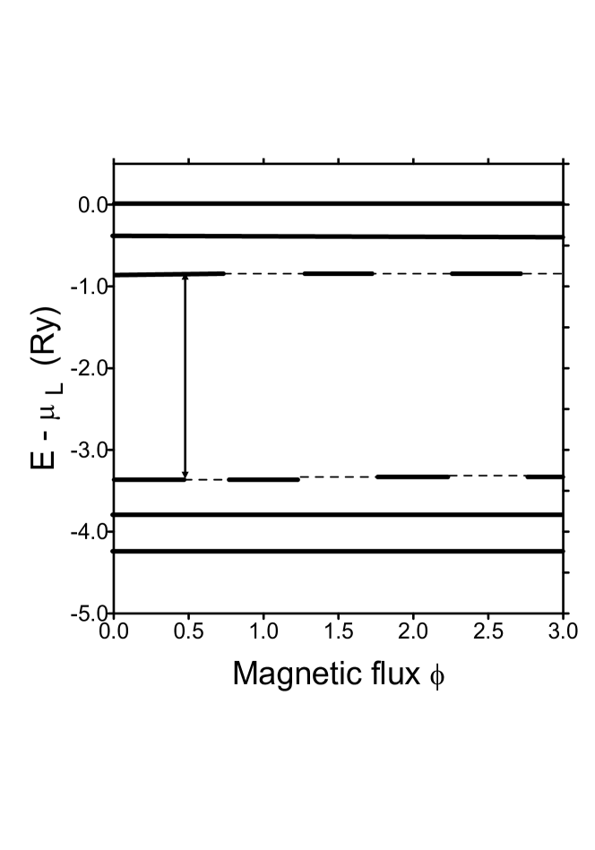
Figure 9: Qualitative scheme of the current passing through the TQD filled with $N$ electrons extracted from the Hubbard results. Thick solid lines correspond to a large tunneling current while thin-dotted lines correspond to a small current under the spin blockade condition.

References

- Awschalom et al. (2002) D. D. Awschalom, D. Loss, and N. Samarth, eds., Semiconductor Spintronics and Quantum Computation, vol. XVI of Series on Nanoscience and Technology (Springer, New York, 2002).
- Brum and Hawrylak (1997) J. A. Brum and P. Hawrylak, Superlattices Microstruct. 22, 431 (1997).
- Loss and DiVincenzo (1998) D. Loss and D. P. DiVincenzo, Phys. Rev. A 57, 120 (1998).
- DiVincenzo et al. (2000) D. P. DiVincenzo, D. Bacon, J. Kempe, G. Burkard, and K. B. Whaley, Nature 408, 339 (2000).
- A.S. Sachrajda and Ciorga (2003) P. H. A.S. Sachrajda and M. Ciorga, Nano-spintronics with lateral quantum dots (ed. by J. P. Bird, Kluwer Academic Publishers, Boston, 2003).
- Ciorga et al. (2000) M. Ciorga, A. S. Sachrajda, P. Hawrylak, C. Gould, P. Zawadzki, S. Jullian, Y. Feng, and Z. Wasilewski, Phys. Rev. B 61, R16315 (2000).
- Tarucha et al. (1996) S. Tarucha, D. G. Austing, T. Honda, R. J. van der Hage, and L. P. Kouwenhoven, Phys. Rev. Lett. 77, 3613 (1996).
- Holleitner et al. (2002) A. W. Holleitner, R. H. Blick, A. K. Hüttel, K. Eberl, and J. P. Kotthaus, Science 297, 70 (2002).
- Pioro-Ladriere et al. (2005) M. Pioro-Ladriere, R. Abolfath, P. Zawadzki, J. Lapointe, S. Studenikin, A. S. Sachrajda, and P. Hawrylak, Phys. Rev. B 72, 125307 (2005).
- Koppens et al. (2005) F. H. Koppens, J. A. Folk, J. M. Elzerman, R. Hanson, L. H. W. van Beveren, I. T. Vink, H. P. Tranitz, W. Wegscheider, L. P. Kouwenhoven, and L. M. K. Vandersypen, Science 309, 1346 (2005).
- Petta et al. (2005) J. R. Petta, A. C. Johnson, J. M. Taylor, E. A. Laird, A. Yacoby, M. D. Lukin, C. M. Marcus, M. P. Hanson, and A. C. Gossard, Science 309, 2180 (2005).
- Hatano et al. (2005) T. Hatano, M. Stopa, and S. Tarucha, Science 309, 268 (2005).
- Vidan et al. (2004) A. Vidan, R. M. Westervelt, M. Stopa, M. Hanson, and A. C. Gossard, Appl. Phys. Lett. 85, 3602 (2004).
- Vidan et al. (2005) A. Vidan, R. M. Westervelt, M. Stopa, M. Hanson, and A. C. Gossard, J. Supercond. 18, 223 (2005).
- Gaudreau et al. (2006) L. Gaudreau, S. Studenikin, A. Sachrajda, P. Zawadzki, A. Kam, J. Lapointe, M. Korkusinski, and P. Hawrylak, Phys. Rev. Lett. 97, 036807 (2006).
- Ihn et al. (2007) T. Ihn, M. Sigrist, K. Ensslin, W. Wegscheider, and M. Reinwald, New J. Phys. 9, 111 (2007).
- Korkusinski et al. (2007) M. Korkusinski, I. Puerto Gimenez, P. Hawrylak, L. Gaudreau, S. A. Studenikin, and A. S. Sachrajda, Phys. Rev. B 75, 115301 (2007).
- Gaudreau et al. (2007) L. Gaudreau, A.S.Sachrajda, S.Studenikin, P.Zawadzki, A.Kam, and J. Lapointe, ICPS Conf. Proc., to be published (2007).
- Scarola and DasSarma (2005) V. W. Scarola and S. DasSarma, Phys. Rev. A 71, 032340 (2005).
- Scarola et al. (2004) V. W. Scarola, K. Park, and S. Das Sarma, Phys. Rev. Lett. 93, 120503 (2004).
- Hawrylak and Korkusinski (2005) P. Hawrylak and M. Korkusinski, Solid State Commun. 136, 508 (2005).
- Stopa et al. (2006) M. Stopa, A. Vidan, T. Hatano, S. Tarucha, and R. M. Westervelt, Physica E 34, 616 (2006).
- Kuzmenko et al. (2002) T. Kuzmenko, K. Kikoin, and Y. Avishai, Phys. Rev. Lett. 89, 156602 (2002).
- Kuzmenko et al. (2006) T. Kuzmenko, K. Kikoin, and Y. Avishai, Phys. Rev. Lett. 96, 046601 (2006).
- (25) K.Kikoin and Y. Avishai, cond-mat/0612028.
- Jiang and Sun (2007) Z.-T. Jiang and Q.-F. Sun, J. Phys.: Condens. Matter 19, 156213 (2007).
- (27) C. Emary, cond-mat/0705.2934.
- Peierls (1933) R. Peierls, Z. Phys. 80, 763 (1933).
- Luttinger (1951) J. M. Luttinger, Phys. Rev. 84, 814 (1951).
- Abolfath and Hawrylak (2007) R. M. Abolfath and P. Hawrylak, Phys. Rev. Lett. 97, 186802 (2007).
- Hawrylak (1993) P. Hawrylak, Phys. Rev. Lett. 71, 3347 (1993).