Analytic theory of narrow lattice solitons

Abstract

The profiles of narrow lattice solitons are calculated analytically using perturbation analysis. A stability analysis shows that solitons centered at a lattice (potential) maximum or saddle point are unstable, as they drift toward the nearest lattice minimum. This instability can, however, be so weak that the soliton is “mathematically unstable” but “physically stable”. Stability of solitons centered at a lattice minimum depends on the dimension of the problem and on the nonlinearity. In the subcritical and supercritical cases, the lattice does not affect the stability, leaving the solitons stable and unstable, respectively. In contrast, in the critical case (e.g., a cubic nonlinearity in two transverse dimensions), the lattice stabilizes the (previously unstable) solitons. The stability in this case can be so weak, however, that the soliton is “mathematically stable” but “physically unstable”.

1 Introduction

Solitons are localized waves that propagate in nonlinear media where dispersion and/or diffraction are present. They appear in various fields of physics such as nonlinear optics, Bose-Einstein Condensates (BEC), plasma physics, solid state physics and water waves. The dynamics of solitons is modeled by the Nonlinear Schrödinger equation (NLS) in the context of nonlinear optics which is also known as the Gross-Pitaevskii (GP) equation in the context of BEC.

In the study of stability of solitons in a homogeneous medium, it is useful to consider the $d$-dimensional focusing NLS

$$iA_{z}(z,{\bf x})\ =\ -\nabla^{2}A-|A|^{p-1}A,$$ (1)

where $z$ is the longitudinal coordinate, ${\bf x}=(x_{1},\dots,x_{d})$ are the coordinates in the transverse plane, $\nabla^{2}=\partial_{{x_{1}}{x_{1}}}+\cdots+\partial_{{x_{d}}{x_{d}}}$ is the Laplacian operator and the nonlinearity is focusing with exponent $p>1$. In optics, the $z$ variable in Eq. (1) is normalized by $2L_{diff}$, where $L_{diff}$ is the diffraction (Rayleigh) length and the $x_{j}$ variables are normalized by the input beam radius.

We delineate several cases for the NLS (1):

$$0\ <\ p-1\ <\ \frac{4}{d},\ \ \ {\rm the\ subcritical\ case},$$ (2)

$$p-1\ =\ \frac{4}{d},\ \ \ {\rm the\ critical\ case,}$$

$$p-1\ >\ \frac{4}{d},\ \ \ {\rm the\ supercritical\ case}.$$

In the subcritical case, the solitary waves $A=e^{i\nu z}u_{\nu}({\bf x})$ of the NLS (1) are stable, while in the critical and supercritical cases the solitary waves of the NLS (1) are unstable. The profile of a stable solitary wave experiences only minor changes under small perturbations as it propagates. On the other hand, unstable solitary waves can change dramatically due to the effect of an infinitesimal perturbation. For the NLS (1), unstable solitary waves either collapse after propagating a finite distance, or diffract as $z$ goes to infinity [1, 2].

Solitons have been thoroughly studied in view of their potential application in optical communications and switching devices (in nonlinear optics) or in quantum information science (in BEC). Recent advances in fabrication and experimental methods now make possible the realization of transparent materials with spatially varying, high contrast dielectric properties. Such materials have various all-optical signal processing applications in optical communications, see e.g. [3, 4]. In this case, the solitons are usually called lattice solitons. Specifically, by a proper design of the dielectric properties of the medium, it may be possible to avoid the blowup/diffraction instability in the critical and supercritical cases and to obtain stable propagation of laser beams in those structures [5, 6, 7, 8]. Thus, there is considerable interest in understanding the propagation of light in modulated media.

Most studies of such media have considered linear lattices (potentials). In this case, the equation of propagation is

$$iA_{z}(z,{\bf x})=-\nabla^{2}A-|A|^{p-1}A+V(N{\bf x}_{lat})A,$$ (3)

where ${\bf x}_{lat}=(x_{1},\dots,x_{d_{lat}})$ are the lattice coordinates, $1\leq d_{lat}\leq d$ is the lattice dimension and $1/N$ is the characteristic length-scale of change of the lattice. For example, if the lattice is periodic, then $N$ is the lattice period. In the context of nonlinear optics, linear potentials are created by modulating the linear refractive index $n_{0}$ in space. If the modulation/potential is periodic, such structures are called waveguide arrays or photonic lattices. In the context of BEC, the corresponding Gross-Pitaevskii equation accounts for the interaction of the atoms with a magnetic trap or, in the case of a periodic optical lattice, with interfering laser beams, see [9, 10] and references therein.

Solitary waves of the NLS (3) with a general linear potential were studied in [11, 12], to name a few of the earlier studies. Recently, many studies considered periodic potentials. Theoretical and numerical studies of solitons of the NLS/GP equation were done for a periodic potential in one [13, 14, 15, 16], two [17, 18, 19] and three [20, 21] dimensions. Experimental realization of these solitons were obtained in one-dimensional waveguide arrays [22] and in two-dimensional optically induced photonic lattices in photorefractive media [23, 24, 25, 26, 27]. Some studies also involved lattices whose dimensionality is smaller than the spatial dimension, i.e., $d_{lat}<d$ (see e.g. [8, 28]) and in media with a quintic nonlinearity (see [29] and references therein).

Generally speaking, it was found that for some lattice types and propagation constants $\nu$, the lattice can prevent the collapse and stabilize the solitons in the critical and supercritical cases. However, the possibility that these stable solitons can collapse under a sufficiently large perturbation was not mentioned in previous studies.

A detailed study of stability (and collapse) of solitons in a nonlinear lattice, i.e.,

$$iA_{z}(z,{\bf x})=-\nabla^{2}A-V(N{\bf x}_{lat})|A|^{p-1}A,$$ (4)

was done in [30, 31]. In these studies it was shown that the soliton profile and (in)stability properties strongly depend on whether it is wider than, of the same order of, or narrower than the lattice period. Specifically, it has been shown that the same nonlinear lattice may stabilize beams of a certain width while destabilizing beams of a different width. Hence, any study of the stability of lattice solitons should take into account the (relative) soliton width.

In this paper, we conduct a systematic study of the stability and instability dynamics of solitons in linear lattices which are narrow with respect to the lattice period. The fact that the solitons are narrow imply that there is a small non-dimensional parameter ${\tilde{N}}$, see Eq. (6). This allows us to employ perturbation methods and to compute the soliton profile and related quantities (soliton power, perturbed zero-eigenvalues $\lambda_{0,j}^{(N)}$, see below) asymptotically.

In nonlinear optics, typical lattice periods are of the order of several microns and typical input beam sizes are not smaller than this period [22, 25, 32, 33, 6]. Hence, typically, the input beam sizes are not small compared with the lattice period. However, if the beam undergoes collapse, the beam can become much narrower than the lattice period. In BEC, the standard magnetic traps are significantly wider than the size of the condensate. Hence, the narrow beams limit is of physical relevance. From a theoretical point of view, the limit of narrow beams corresponds to the semi-classical limit of the nonlinear Schrödinger equation

$$ihA_{z}(z,{\bf x})=-h^{2}\nabla^{2}A-|A|^{p-1}A+V({\bf x}_{lat})A,\quad\quad h\longrightarrow 0,$$ (5)

see e.g., [11, 34]. Moreover, as discussed in Section 6, in many cases, the results for narrow beams hold also for beams of ${\cal O}(1)$ width.

The paper is organized as follows: In Section 2, we present various physical models in nonlinear optics and in BEC where Eq. (3) arises. In Section 3, the equation for lattice soliton is derived. It is shown that the soliton width is given by a single parameter

$${\tilde{N}}=\frac{N}{\sqrt{\eta}}\ll 1,\quad\quad\eta=\nu+V(0),$$ (6)

where $V(0)$ is the potential at the soliton center. Therefore, the limit $\nu\to\infty$ analyzed in [35], and the limit $N\to 0$ analyzed in [34], are in fact the same limit. It is well known that narrow solitons of a periodic lattice are found deep inside the “semi-infinite gap” of the linear problem, away from the first band of the allowed solutions [15], i.e., for $\nu\to\infty$. Indeed, in this case ${\tilde{N}}\to 0$. However, from this argument it is not clear how large should $\nu$ be in order for the soliton to be narrow. This information is given by the parameter ${\tilde{N}}$, which is thus, a more informative parameter than the propagation constant $\nu$. Moreover, the parameter ${\tilde{N}}$ includes also the effect of the lattice strength on the width and reflects the fact that as $V(0)$ increases, the beam confinement increases, hence the beam becomes narrower .

In Section 3, we also use perturbation analysis to calculate the profile of narrow lattice solitons for any dimension $d$, lattice dimensionality $d_{lat}$ and nonlinearity exponent $p$. As can be expected, this calculation shows that the soliton profile depends only on the local properties of the lattice, rather than on the full lattice structure. Hence, our study is relevant to any slowly varying lattice, regardless of its long-scale properties. To simplify the notation, we mostly consider lattices that are aligned in the directions of the Cartesian axes. In this case, the lattice can be expanded as

$$V(N{\bf x}_{lat})=V(0)+\eta\left(N^{2}\sum_{j=1}^{d_{lat}}v_{jj}x^{2}_{j}+{\cal O}({\tilde{N}}^{4})\right).$$ (7)

Our results are valid, however, to any linear lattice, see Remark 3.1.

In Section 4, we analyze the stability of narrow lattice solitons. We first present the two conditions for stability of lattice solitons in Theorem 4.1. The first condition, known as the Vakhitov-Kolokolov condition [36] or the slope condition [37], is that the power (or $L_{2}$ norm) of the soliton should increase with $\nu$. Using the results of the perturbation analysis, we show in Section 4.1 that to leading order, the power of a narrow lattice soliton is equivalent to the power of a soliton in a homogeneous medium, and that the change in the power due to the lattice scales as ${\tilde{N}}^{2}$.  In particular, the lattice causes the power to decrease (increase) for lattice solitons centered at a lattice minimum (maximum). In addition, the power curve slope is more positive (negative) for lattice solitons centered at a lattice minimum (maximum). Since in a homogeneous medium the slope has an ${\cal O}(1)$ magnitude in the subcritical and supercritical cases, the small change of the slope by the lattice does not affect the sign of the slope. Accordingly, the slope condition remains satisfied in the subcritical case and violated in the supercritical case. In the critical case, the slope in a homogeneous medium is zero. As a result, the ${\cal O}({\tilde{N}}^{2})$ change in the power by the lattice leads to a positive (negative) slope for lattice solitons centered at a lattice minimum (maximum). Hence, the slope condition is satisfied for narrow lattice solitons centered at a lattice minimum, but is “even more” violated for lattice solitons centered at a lattice maximum.

The second condition for stability of narrow lattice solitons is the spectral condition [39], and it involves the number of negative eigenvalues of the linearized operator $L^{(N)}_{+,\nu}$, see Eq. (37). In Section 4.2, we first show that the spectral condition is violated if and only if the lattice causes some of the zero eigenvalues of the homogeneous medium linearized operator $L_{+,\nu}$ (see Eq. (45)) to become negative. Then, we use a perturbation analysis to show that the values of the perturbed zero eigenvalues $\lambda_{0,j}^{(N)}$ are given by

$$\lambda_{0,j}^{(N)} = \left\{\begin{array}[]{llll}\delta v_{jj}N^{2}+{\cal O}({\tilde{N}}^{4}),&&&j=1,\dots,d_{lat},\\ 0,&&&j=d_{lat}+1,\dots,d,\end{array}\right.$$ (10)

where

$$\delta = \frac{p(2-d)+2+d}{p-1},$$

see Lemma 4.2. This calculation shows that the eigenvalues become positive (negative) for solitons centered at a lattice minimum (maximum). Hence, the spectral condition is satisfied (violated) for solitons centered at a lattice minimum (maximum). This calculation generalizes the result of Oh in the one-dimensional cubic case [11] to any dimension $d$, any lattice dimension $d_{lat}$ and any nonlinearity exponent $p$.

In order to test the validity of the analytical formula for $\lambda_{0,j}^{(N)}$, we also compute these eigenvalues numerically. For $d\geq 2$, the matrix that represents the linearized operator $L_{+,\nu}^{(N)}$ is very large. As a result, standard numerical schemes (e.g., Matlab’s eig or eigs) usually fail to compute its eigenvalues. In order to overcome this numerical difficulty, we use a numerical scheme which is based on the Arnoldi algorithm, see C. While in this study we “only” use this scheme to verify the validity of the analytical approximation of the eigenvalue, we note that in the case of non-narrow lattice solitons, the eigenvalue cannot be computed analytically, and the only way to check the spectral condition is numerically. Moreover, this numerical scheme can be used in similar eigenvalue problems in which large matrices are involved.

Combining the results of Sections 4.1 and 4.2, we show in Section 4.3 (Proposition 4.2) that in the subcritical and critical cases, narrow lattice solitons are stable when centered at a lattice minimum, and unstable when centered at a lattice maximum or at a saddle point. In the supercritical case, narrow lattice solitons are unstable at both lattice maxima and minima.

Proposition 4.2 specifies when the two conditions for stability are violated. It does not, however, describe the resulting instability dynamics. The relations between the condition which is violated and the instability dynamics were observed in [30, 31] for a nonlinear lattice and in [40] for a linear delta-potential to be as follows:

1. if the slope is negative, the soliton width can undergo significant changes. In the critical and supercritical cases, this width instability can result in collapse. In the subcritical case, this width instability can “only” result in a “finite-width” instability, i.e., the soliton width can decrease substantially, but not to zero.

2. When the spectral condition is violated, the solitons undergo a drift instability, i.e., the soliton drifts away from the lattice maximum towards the nearest lattice minimum.

3. When both conditions for stability are violated, a combination of a width instability and a drift instability can be observed.

In the case of narrow lattice solitons, the slope is always positive in the subcritical case. Hence, the instability due to a negative slope is a blowup instability and not a “finite-width” instability. Furthermore, in Section 4.4 we prove that when the spectral condition is violated (i.e., if the soliton is centered at a lattice maximum or saddle point), narrow lattice solitons undergo a drift instability, i.e., they move away from their initial location at an exponential drift-rate. In contrast, solitons centered near a lattice minimum (for which the spectral condition is satisfied) undergo small oscillations around the lattice minimum. The above observations on the condition leading to instability and the type of instability dynamics are summarized in Table 1.

	lattice minimum	lattice maximum
Subcritical	Stability	Instability† (drift)
Critical	Stability	Instability∗,† (blowup+drift)
Supercritical	Instability∗ (blowup)	Instability∗,† (blowup+drift)

Table 1: Stability of narrow lattice solitons. Condition leading to instability is marked by ^∗ for a failure to satisfy the slope condition and by ^† for a failure to satisfy the spectral condition. In the case of instability, its dynamics is indicated in parentheses.

In Section 5, we study the dynamics of solitons in the two cases where the small effect of the lattice changes the stability. As observed in [30, 31], in such cases, it is important to study both stability and instability quantitatively. In Section 5.1, we discuss the strength of the stabilization induced by the lattice for solitons centered at a lattice minimum in the critical case. To do so, we use the concept of the stability region, i.e., the region in function space of initial conditions around the soliton profile that lead to a stable propagation. As in the case of a nonlinear lattice [30, 31], our results indicate that the ${\cal O}({\tilde{N}}^{2})$ small slope of the power curve implies that the stability region is ${\cal O}({\tilde{N}}^{2})$ small . Therefore, although the two conditions for stability are satisfied, these solitons can become unstable under extremely small perturbations. Practically, this means that in the critical case, “mathematically” stable solutions can be “physically” unstable i.e., become unstable under typical physical perturbations. We illustrate these results using two standard types of lattices: A sinusoidal potential, which is typical in photorefractive materials [23, 25] and in BEC [41] and a Kronig-Penney step lattice (periodic array of finite potential wells) [42], which is typical for manufactured slab waveguide arrays, see e.g., [13, 22, 33]. We study numerically the stability of solitons under random perturbations that either increase or decrease the total power of the soliton and observe that narrow lattice solitons are “mathematically” stable but “physically” unstable. The stability is particularly weak for Kronig-Penney lattice solitons, for which the slope is exponentially small. In addition, we observe that when the perturbation is sufficiently “non-small”, both the sinusoidal and KP (stable) lattice solitons can undergo a blowup instability. This shows that in the absence of translation invariance, stability and blowup can coexist in NLS equations [30, 31, 43].

In Section 5.2, we show that the opposite scenario is also possible, i.e., “mathematically unstable” solitons can be “physically stable”. This occurs for subcritical narrow lattice solitons centered at a lattice maximum, which are unstable due to a violation of the spectral condition (Proposition 4.2). We show that the drift rate is exponential in $\bigg{(}-\lambda_{0}^{(N)}\bigg{)}^{1/2}$. Therefore, narrow solitons, for which $\lambda_{0}^{(N)}$ is ${\cal O}(N^{2})$ small, experience very slow drift and can thus be “stable” for the distances/times in experimental setups. In particular, we observe that the Kronig-Penney lattice soliton drifts much more slowly than the sinusoidal lattice soliton of the same width. Section 6 concludes with some concluding remarks.

2 Physical models

We consider the d dimensional NLS equation (3) with a linear lattice in $d_{lat}$ dimensions ($1\leq d_{lat}\leq d$). This model describes numerous physical configurations. For example, beam propagation in a Kerr slab waveguide with a lattice is modeled by

$$iA_{z}(z,x)=-A_{xx}-|A|^{2}A+V(Nx)A.$$ (11)

In this case, $p=3$, $d=d_{lat}=1$, ${\bf x}={\bf x_{lat}}=x$ and $V=V(Nx)$, see e.g., [44, 15, 22]. Beam propagation in bulk Kerr medium with a two-dimensional lattice is modeled by

$$iA_{z}(z,x,y)=-\nabla^{2}A-|A|^{2}A+VA.$$ (12)

In this case, $p=3$, $d=2$ and ${\bf x}=(x,y)$. If $V=V(Nx,Ny)$, then $d_{lat}=2$, and ${\bf x}_{lat}=(x,y)$, see e.g., [18, 19, 17]; if $V=V(Nx)$ then $d_{lat}=1$, and ${\bf x}_{lat}=x$. In the latter case, the dimension of the lattice $d_{lat}$ is smaller by one from the dimension of the transverse space $d$, see e.g., [8, 31, 28].

Propagation of ultrashort pulses in a slab waveguide is modeled by

$$iA_{z}(z,x,t)=-A_{xx}+\beta_{2}A_{tt}-|A|^{2}A+V(Nx)A,$$ (13)

where $\beta_{2}$ is the group velocity dispersion (GVD) parameter. In the case of anomalous dispersion ($\beta_{2}<0$), the time coordinate $t$ is effectively an additional transverse dimension. Then, Eq. (13) corresponds to Eq. (3) with $p=3$, $d=2$, ${\bf x}=(x,t)$, $d_{lat}=1$ and ${\bf x}_{lat}=x$, so the dimension of the lattice $d_{lat}$ is smaller by one from the dimension of the transverse space $d$, see e.g., [8, 31]. Similarly, propagation of ultrashort pulses in a 2D optical lattice is modeled by

$$iA_{z}(z,x,y,t)=-\nabla^{2}A+\beta A_{tt}-|A|^{2}A+VA,$$ (14)

which for $\beta<0$ corresponds to Eq. (3) with $p=3$, $d=3$ and ${\bf x}=(x,y,t)$. If $V=V(Nx,Ny)$, then $d_{lat}=2$, and ${\bf x}_{lat}=(x,y)$ [21]; if $V=V(Nx)$ then $d_{lat}=1$, and ${\bf x}_{lat}=x$.

The linear lattice $V$ in Eq. (3) varies in the transverse coordinates but not in $z$. In some applications, the lattice varies in the direction of propagation $z$. Such problems, however, will not be studied in this paper.

Eq. (3) also models the dynamics of Bose-Einstein condensates (BEC) with a negative scattering length. In this case, $z$ is replaced with $t$. In BEC, typically ${\bf x}=(x,y,z)$, i.e., $d=3$, but under certain conditions the cases $d=1$ and $d=2$ are also of physical interest, see e.g., [45, 46]. The exponent $p$ is usually equal to $3$ but can also be equal to $5$, see [29] and references therein. In the BEC context, both a parabolic potential and a periodic potential appear in the experimental setups [9].

3 Narrow lattice solitons

We look for lattice solitons, which are of solutions of Eq. (3) of the form

$$A(z,{\bf x})=e^{i\nu z}u_{\nu}^{(N)}({\bf x}),\quad\quad\nu>0,$$ (15)

where $u_{\nu}^{(N)}$ is the solution of

$$\nabla^{2}u_{\nu}^{(N)}({\bf x})+\big{(}u_{\nu}^{(N)}\big{)}^{p}-[\nu+V(N{\bf x}_{lat})]u_{\nu}^{(N)}=0.$$ (16)

We consider lattices which are symmetric with respect to a critical point ${\bf x}_{lat}^{(0)}$ of the lattice $V$. Hence, the soliton maximal amplitude is attained at ${\bf x}_{lat}^{(0)}$ [47]. The boundary conditions for Eq. (16) are $\nabla u_{\nu}^{(N)}({\bf x}_{lat}^{(0)})=0$ and $u_{\nu}^{(N)}(\infty)=0$. Without loss of generality, we set ${\bf x}_{lat}^{(0)}=0$.

We study solutions of Eq. (16) which are narrow with respect to the lattice characteristic length-scale. A priori, the relative width of a lattice depends on the lattice strength, the lattice period (or characteristic length) $1/N$ and the propagation constant $\nu$. We now show that in the case of narrow solitons, one can rescale Eq. (16) to a form where the relative width of the beam is given by a single parameter ${\tilde{N}}$. In order to achieve that, we define

$$\eta=\nu+V(0),\quad\quad{\tilde{N}}=N/\sqrt{\eta},\quad\quad u_{\nu}^{(N)}({\bf x})=\eta^{\frac{1}{p-1}}u_{{\tilde{N}}}(\sqrt{\eta}{\bf x}).$$ (17)

Then, Eq. (16) becomes

$$\nabla^{2}u_{\tilde{N}}(\tilde{\bf x})+u_{\tilde{N}}^{p}-[1+\tilde{V}({\tilde{N}}\tilde{\bf x}_{lat})]u_{\tilde{N}}=0,\quad\nabla u_{\tilde{N}}(0),\quad u_{\tilde{N}}(\infty)=0,$$ (18)

where

$$\tilde{\bf x}=\sqrt{\eta}{\bf x},\quad\quad\tilde{\bf x}_{lat}=\sqrt{\eta}{\bf x}_{lat},\quad\quad\tilde{V}({\tilde{N}}\tilde{\bf x}_{lat})=\frac{V({\tilde{N}}\tilde{\bf x}_{lat})-V(0)}{\eta}.$$ (19)

When ${\tilde{N}}\ll 1$, we can expand the solution of Eq. (18) as a power series of ${\tilde{N}}^{2}$, i.e.,

$$u_{\tilde{N}}(\tilde{\bf x})={\cal U}(|\tilde{\bf x}|)+{\tilde{N}}^{2}g(\tilde{\bf x})+{\cal O}({\tilde{N}}^{4}),$$ (20)

where ${\cal U}$ is the positive, radially-symmetric ground-state solution of

$$\nabla^{2}{\cal U}(|\tilde{\bf x}|)+{\cal U}^{p}-{\cal U}=0.$$ (21)

Similarly, since $\tilde{V}(0)=0$ and $\nabla\tilde{V}(0)=0$, the potential $\tilde{V}({\tilde{N}}\tilde{\bf x}_{lat})$ can be expanded for ${\tilde{N}}\ll 1$ as

$$\tilde{V}({\tilde{N}}\tilde{\bf x}_{lat})={\tilde{N}}^{2}\tilde{V}_{2}(\tilde{\bf x}_{lat})+{\cal O}({\tilde{N}}^{4}),$$ (22)

where

$$\tilde{V}_{2}(\tilde{\bf x}_{lat})=\sum_{j,k=1}^{d_{lat}}v_{jk}\tilde{x}_{j}\tilde{x}_{k},\quad\quad v_{jk}=\frac{1}{2}\frac{\partial^{2}\tilde{V}({\bf y}_{lat})}{\partial{y_{j}}\partial{y_{k}}}\bigg{|}_{{\bf y}_{lat}=0},$$ (23)

is the first non-vanishing term in the Taylor expansion of $\tilde{V}$ which represents the local curvature of the lattice at the soliton center. In particular, $\tilde{V}_{2}(\tilde{\bf x}_{lat})\geq 0$ ($\leq 0$) for lattice solitons centered at a lattice minimum (maximum).

Remark 3.1

In order to simplify the presentation, we assume that the principle axes of the lattice identify with the Cartesian axes $\{\hat{e}_{1},\dots,\hat{e}_{d_{lat}}\}$. In this case, $v_{jk}=0$ for $j\neq k$,

$$\tilde{V}_{2}(\tilde{\bf x}_{lat})=\sum_{j=1}^{d_{lat}}v_{jj}\tilde{x}_{j}^{2},$$ (24)

and

$$V(N{\bf x}_{lat})=V(0)+\eta\left(N^{2}\sum_{j=1}^{d_{lat}}v_{jj}x^{2}_{j}+{\cal O}({\tilde{N}}^{4})\right),$$ (25)

see Eq. (69). However, all our results can be immediately generalized to the case when the lattice is not aligned along the cartesian axes as follows. Since $v_{jk}=v_{kj}$, there exists a basis of vectors $\{\hat{\epsilon}_{1},\dots,\hat{\epsilon}_{d_{lat}}\}$ such that if $\tilde{\bf x}_{lat}=\sum_{j=1}^{d_{lat}}\alpha_{j}\hat{\epsilon}_{j}$ then

$$\tilde{V}_{2}(\tilde{\bf x}_{lat})=\sum_{j=1}^{d_{lat}}u_{jj}\alpha_{j}^{2}.$$ (26)

Therefore, in order to apply our results to the lattice (23), one needs to replace $x_{j}$ by $\alpha_{j}$ and $v_{jj}$ by $u_{jj}$. See e.g., Remark 3.2 and Remark 4.1.

Using a perturbation analysis similar to the one used in [30, 38], we show that

Lemma 3.1

The solution of Eq. (18) for ${\tilde{N}}\ll 1$ is given by

$$u_{\tilde{N}}(\tilde{\bf x})={\cal U}(|\tilde{\bf x}|)-{\tilde{N}}^{2}L_{+}^{-1}\left(\tilde{V}_{2}(\tilde{\bf x}_{lat}){\cal U}\right)+{\cal O}({\tilde{N}}^{4}),$$ (27)

where ${\cal U}$ is given by Eq. (21), $\tilde{V}_{2}$ is given by Eq. (24) and

$$L_{+}=-\nabla^{2}_{\bf\tilde{x}}-p{\cal U}^{p-1}+1.$$ (28)

Proof: See A.

In the original variables, the expansion (27) becomes

$$u_{\nu}^{(N)}({\bf x}) = (\nu+V(0))^{\frac{1}{p-1}}\left[{\cal U}(\sqrt{\nu+V(0)}|{\bf x}|)+{\cal O}({\tilde{N}}^{2})\right]={\cal U}_{\eta}(|{\bf x}|)+{\cal O}({\tilde{N}}^{2}),$$ (29)

where ${\cal U}_{\eta}=\eta^{\frac{1}{p-1}}{\cal U}(\sqrt{\eta}|\tilde{\bf x}|)$ is the solution of

$$\nabla^{2}{\cal U}_{\eta}(|{\bf x}|)+{\cal U}_{\eta}^{p}-\eta{\cal U}_{\eta}=0.$$ (30)

This expansion shows that:

1. To leading order, a (rescaled) narrow lattice soliton $u_{\tilde{N}}$ is given by the rescaled homogeneous medium soliton ${\cal U}$.

2. The deviation of a narrow lattice soliton $u_{\tilde{N}}$ from ${\cal U}$ is ${\cal O}({\tilde{N}}^{2})$ small, even if the lattice has ${\cal O}(1)$ variations.

The above results also show that the soliton relative width is given by a single parameter ${\tilde{N}}$:

Proposition 3.1

Lattice solitons are narrow with respect to the lattice period if

$${\tilde{N}}=\frac{N}{\sqrt{\eta}}=\frac{N}{\sqrt{\nu+V(0)}}\ll 1.$$ (31)

In this case,

$${\tilde{N}}=\frac{\mbox{soliton width}}{\mbox{lattice period}}.$$ (32)

Proof: By Eq. (27), when ${\tilde{N}}\ll 1$, then $u_{\tilde{N}}$ has ${\cal O}(1)$ width in ${\bf\tilde{x}}$. Hence, by Eq. (29), the width of $u_{\nu}^{(N)}({\bf x})$ in ${\bf x}$ is ${\cal O}(1/\sqrt{\eta})$. Since that the lattice length-scale/period is $1/N$, then the relative width of the soliton is given by ${\tilde{N}}$. $\Box$

We emphasize that the expansion (27) applies to all types of lattices so long as $v_{jj}{\tilde{N}}^{2}\ll 1$. Specifically, for a strong periodic lattice ($V\gg 1$), for which the linear coupling between adjacent lattice sites is weak, the result (29) is still valid provided that ${\tilde{N}}$ is small enough, i.e., for ${\tilde{N}}\ll v_{jj}^{-\frac{1}{2}}$. In that case, the solution (29) is the continuous analog of the discrete solitons of the DNLS model [13, 22, 48].

3.1 Effect of lattice type

Lemma 3.1 shows that the effect of the lattice depends on whether $\tilde{V}_{2}\not\equiv 0$ or $\tilde{V}_{2}\equiv 0$. When $\tilde{V}_{2}\not\equiv 0$, then the lattice effect is ${\cal O}({\tilde{N}}^{2})$. This case corresponds to a parabolic lattice, a sinusoidal lattice etc. However, when $\tilde{V}_{2}\equiv 0$, then $g({\bf x})\equiv 0$ and the next-order term in the expansion (20) must be considered. In particular, in the special case of a Kronig-Penney step lattice (see, e.g., Eq. (41)), all derivatives of $\tilde{V}$ at the soliton center ${\bf x}_{lat}^{(0)}=0$ vanish. Therefore, the difference between $u_{\tilde{N}}$ and ${\cal U}$ will be exponentially small.

3.2 Effect of lattice inhomogeneity on soliton profile

In order to calculate the effect of the lattice on the soliton profile, we note that

$$L_{+}^{-1}\left(\tilde{x}_{j}^{2}{\cal U}\right)=\tilde{x}_{j}^{2}S(|\tilde{\bf x}|)+Q(|\tilde{\bf x}|),$$ (33)

where $S$ and $Q$ are radial functions which are the solutions of

$$L_{+}S-\frac{4}{\tilde{r}}S^{\prime}={\cal U},\quad\quad L_{+}Q=2S.$$ (34)

Indeed, applying the operator $L_{+}$ to the right-hand-side of Eq. (33) gives

$$L_{+}\left(\tilde{x}_{j}^{2}S(|\tilde{\bf x}|)+Q(|\tilde{\bf x}|)\right) = \left(-\nabla^{2}_{\tilde{\bf x}}+1-p{\cal U}^{p-1}\right)\left(\tilde{x}_{j}^{2}S(r)+Q(\tilde{r})\right)$$

$$= \tilde{x}_{j}^{2}\underbrace{\left(L_{+}S(\tilde{r})-\frac{4}{\tilde{r}}S^{\prime}(\tilde{r})\right)}_{={\cal U}}-\underbrace{\left(2S(\tilde{r})+L_{+}Q(\tilde{r})\right)}_{=0}=\tilde{x}_{j}^{2}{\cal U}.$$

Therefore, the ${\cal O}({\tilde{N}}^{2})$ correction to the soliton profile due to the lattice (24) is given by, see Eq. (27),

$$u_{\tilde{N}}-{\cal U}\sim-{\tilde{N}}^{2}L_{+}^{-1}\left(V_{2}(\tilde{\bf x}_{lat}){\cal U}\right)=-{\tilde{N}}^{2}\Big{(}\underbrace{S(|\tilde{\bf x}|)\sum_{j=1}^{d_{lat}}v_{jj}\tilde{x}_{j}^{2}}_{\mbox{anisotropic}}\ \underbrace{+Q(|\tilde{\bf x}|)\sum_{j=1}^{d_{lat}}v_{jj}}_{\mbox{isotropic}}\Big{)}.$$ (35)

Thus, the variation of the lattice in the direction $x_{j}$ has an isotropic effect through $Q(|\tilde{\bf x}|)$ and an anisotropic effect in the direction $x_{j}$ through $S(|\tilde{\bf x}|)$.

Remark 3.2

If $\tilde{V}_{2}$ is given by the lattice (23), then, the ${\cal O}({\tilde{N}}^{2})$ correction to the soliton profile is given by

$$u_{\tilde{N}}-{\cal U}\sim-{\tilde{N}}^{2}L_{+}^{-1}\left(V_{2}(\tilde{\bf x}_{lat}){\cal U}\right)=-{\tilde{N}}^{2}\left(S(|\tilde{\bf x}|)\sum_{j=1}^{d_{lat}}u_{jj}\tilde{\alpha}_{j}^{2}+Q(|\tilde{\bf x}|)\sum_{j=1}^{d_{lat}}u_{jj}\right).$$ (36)

4 Stability and instability of lattice solitons

Eq. (29) implies that narrow lattice solitons $u_{\nu}^{(N)}$ are positive. The conditions for stability and instability of positive lattice solitons are as follows ([30], and see also [49, 37, 39]):

Theorem 4.1

Let $u^{(N)}_{\nu}$ be a positive solution of Eq. (16), let $\mathcal{P}_{\nu}^{(N)}\equiv\int\left(u_{\nu}^{(N)}\right)^{2}d{\bf x}$ be the power of $u_{\nu}^{(N)}$, and let $n_{-}(L^{(N)}_{+,\nu})$ be the number of negative eigenvalues of the linearized operator

$$L_{+,\nu}^{(N)}=-\nabla^{2}+\nu-p\big{(}u^{(N)}_{\nu}({\bf x})\big{)}^{p-1}+V(N{\bf x}_{lat}).$$ (37)

Then, the lattice soliton $A(z,{\bf x})=e^{i\nu z}u_{\nu}^{(N)}({\bf x})$ is

1. an orbitally stable solution of Eq. (3) if

   1. $\partial_{\nu}\mathcal{P}^{(N)}_{\nu}>0$ (slope condition), and

   2. $n_{-}(L^{(N)}_{+,\nu})=1$ (spectral condition).

2. an orbitally unstable solution of Eq. (3) if

   1. $\partial_{\nu}\mathcal{P}^{(N)}_{\nu}<0$, or

   2. $n_{-}(L^{(N)}_{+,\nu})>1$.

In what follows, we use the expansion (27) to determine whether the two conditions in Theorem 4.1 are satisfied ,and consequently determine the stability of narrow lattice solitons.

4.1 Slope condition

We can use the expansion (27) to calculate the power of narrow lattice solitons:

Lemma 4.1

The power of narrow lattice solitons (${\tilde{N}}\ll 1$) is given by

$$\mathcal{P}_{\nu}^{(N)} = \left(\nu+V(0)\right)^{\frac{4-d(p-1)}{2(p-1)}}\left(\mathcal{P}_{\nu=1}-C_{V}{\tilde{N}}^{2}\sum_{j=1}^{d_{lat}}v_{jj}+{\cal O}({\tilde{N}}^{4})\right),$$ (38)

where $\mathcal{P}_{\nu=1}=\int\left|{\cal U}\right|^{2}d\tilde{\bf x}$, ${\cal U}$ is the positive solution of Eq. (21), and

$$C_{V}=\frac{2p-6+dp-d}{2d(p-1)}\int|\tilde{\bf x}|^{2}{\cal U}^{2}d\tilde{\bf x}$$ (39)

is a constant independent of $N$ and $\nu$.

Proof: See B.

Eq. (38) shows that, in a similar manner to its effect on the soliton profile, when $\tilde{V}_{2}\not\equiv 0$ (e.g., in the case of a sinusoidal or parabolic lattice), the lattice has an ${\cal O}({\tilde{N}}^{2})$ small effect on the soliton power, even if the lattice itself is not weak. In light of Section 3.1, in the case of a Kronig-Penney step lattice, the effect of the lattice on the power is exponentially small in ${\tilde{N}}$.

¿From Eq. (39) it also follows that $C_{V}>0$ for $p>1+\frac{4}{2+d}$. In particular, for $p=3$, $C_{V}=\frac{1}{2}\int\tilde{r}^{2}{\cal U}^{2}d\tilde{\bf x}>0$. Thus,

Corollary 4.1

If $\tilde{V}_{2}\not\equiv 0$, the lattice causes the power to decrease (increase) for lattice solitons centered at a lattice minimum (maximum) for any $p>1+\frac{4}{2+d}$, and in particular, for a Kerr nonlinearity $p=3$.

In order to demonstrate the result of Lemma 4.1, we solve Eq. (18) numerically with $d=d_{lat}=2$, ${\bf x}={\bf x}_{lat}=(x,y)$ and $p=3$. For convenience, the numerical results shown here are presented for $\eta=1$ (so that $N={\tilde{N}}$, $u_{\nu}^{(N)}=u_{\tilde{N}}$) and for $V(0)=0$ (so that $V=\tilde{V}$). We study two different two-dimensional lattices with a periodic square topology:

1. A 2D sinusoidal lattice given by

   $$V(Nx,Ny)=\pm\frac{1}{2}\left(\sin^{2}(\pi{N}x)+\sin^{2}(\pi{N}y)\right).$$ (40)

2. A 2D Kronig-Penney lattice that consists of an array of primitive cells of size $[-1/N\ 1/N]\times[-1/N\ 1/N]$, each consisting of circular waveguide with abrupt index change between 0 and $1$, i.e.,

   $$V(Nx,Ny)=\left\{\begin{array}[]{ll}0,&\sqrt{x^{2}+y^{2}}<\frac{N}{N_{0}},\quad\quad N_{0}\cong 2.45\\ \pm 1,&\mathrm{otherwise.}\end{array}\right.$$ (41)

In both cases, the plus/minus sign corresponds to a lattice with a minimum/maximum at ${\bf x}_{c}=0$, respectively. The parameters of these lattices were chosen so that both lattices have a period 1, mean value $1/2$ and vary from $0$ to $\pm 1$. The lattices are shown in Fig. 1 for a lattice with a minimum at ${\bf x}_{c}=0$. Note that both lattices are anisotropic in $r=\sqrt{x^{2}+y^{2}}$, and thus, require a full $2$-dimensional treatment. Moreover, since the 2D cubic NLS is critical, $\mathcal{P}_{\nu=1}=\mathcal{P}_{cr}\cong 11.7$, where $\mathcal{P}_{cr}$ is the critical power for collapse in a homogeneous Kerr medium.

In Fig. 2, we show the power of narrow lattice solitons centered at a lattice minimum for both lattices. For $0\leq N\leq 0.1$ there is good agreement between the numerically calculated value of the power of the sinusoidal lattice solitons and the analytical approximation 

$$\mathcal{P}_{\nu}^{(N)} = \mathcal{P}_{\nu=1}-C_{V}{\tilde{N}}^{2}\sum_{j=1}^{d_{lat}}v_{jj}+{\cal O}({\tilde{N}}^{4})\cong 11.7-6.94\cdot 2(2\pi^{2}){\tilde{N}}\cong 11.7-273.8{\tilde{N}}^{2},$$ (42)

which is derived from Lemma 4.1. In particular, the effect of the lattice on the power of the narrow lattice solitons is much more pronounced in the case of a sinusoidal lattice than in the case of a Kronig-Penney lattice.

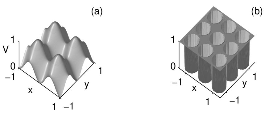
Figure 1: (a) sinusoidal lattice (40) (b) Kronig-Penney lattice (41).

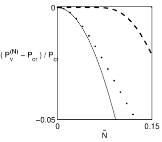
Figure 2: Relative power deviation from $\mathcal{P}_{\nu=1}=\mathcal{P}_{cr}$ for narrow sinusoidal (dots) and Kronig-Penney (dashes) lattice solitons centered at a lattice minimum. The analytical prediction (42) for the sinusoidal lattice is shown by a solid line.

The sign of the slope follows directly from Eq. (38):

Corollary 4.2

Let ${\tilde{N}}\ll 1$. Then, the slope $\partial_{\nu}P_{\nu}^{(N)}$ is positive in the subcritical case ($p<1+4/d$) and negative in the supercritical case ($p>1+4/d$). In the critical case ($p=1+4/d$), the slope is positive for narrow lattice solitons centered at a lattice minimum and negative for narrow lattice solitons centered at a lattice maximum.

Proof: In the subcritical and supercritical cases, the slope is given by

$$\partial_{\nu}\mathcal{P}_{\nu}^{(N)} =\partial_{\nu}\left(\left(\nu+V(0)\right)^{\frac{4-d(p-1)}{2(p-1)}}\left[\mathcal{P}_{\nu=1}+{\cal O}\left(\frac{N^{2}}{\nu+V(0)}\right)\right]\right)$$

$$=\left(\nu+V(0)\right)^{\frac{4-d(p-1)}{2(p-1)}-1}\left[\mathcal{P}_{\nu=1}+{\cal O}\left(\frac{N^{2}}{\nu+V(0)}\right)\right]\sim\left(\nu+V(0)\right)^{\frac{4-d(p-1)}{2(p-1)}-1}\mathcal{P}_{\nu=1}.$$

Therefore, in the subcritical case, the slope is positive while in the supercritical case, the slope is negative. Note that in these cases, the lattice does not affect the sign of the slope.

In the critical case, the first term in Eq. (4.1) vanishes and the slope is determined by the ${\cal O}({\tilde{N}}^{2})$ correction in Eq. (38), i.e.,

$$\partial_{\nu}\mathcal{P}_{\nu}^{(N)} = 0-C_{V}\frac{\partial{\tilde{N}}^{2}}{\partial\nu}\sum_{j=1}^{d_{lat}}v_{jj}+{\cal O}({\tilde{N}}^{4})=2C_{V}\frac{{\tilde{N}}^{2}}{\nu+V(0)}\sum_{j=1}^{d_{lat}}v_{jj}+{\cal O}({\tilde{N}}^{4}),$$ (44)

where we also used Eq. (17). By Eq. (39), in the critical case $C_{V}=\frac{1}{d}\int\tilde{r}^{2}{\cal U}^{2}d\tilde{\bf x}>0$, which completes the proof. $\Box$.

We thus conclude that although the lattice has a small effect on the profile of narrow lattice solitons, in the critical case, this small effect determines the sign of the power slope and hence, the stability (but see Section 5.1).

4.2 Spectral condition

As noted is Section 4, lattice solitons are stable only if in addition to the slope condition, they also satisfy the spectral condition. In the absence of a lattice (i.e., for $V\equiv 0$), the linearized operator $L^{(N)}_{+,\nu}$ reduces to $L_{+,\nu}$ which is given by

$$L_{+,\nu}=-\nabla^{2}-p{\cal U}_{\nu}^{p-1}+\nu,$$ (45)

where ${\cal U}_{\nu}=\nu^{\frac{1}{p-1}}{\cal U}(\sqrt{\nu}|\tilde{\bf x}|)$ and ${\cal U}$ is given by Eq. (21). The spectrum of $L_{+,\nu}$ consists of [49]:

1. A negative eigenvalue $\lambda_{min}$ and a corresponding even and positive eigenfunction $f_{\nu,min}$. In [11], Oh shows that for $d=1$ and $p=3$, $\lambda_{min}=-3\nu$ and $f_{\nu,min}={\cal U}^{2}$. More generally, we observe that for any value of $p$ and $d$,

   $$\lambda_{min}=-\frac{1}{4}\left(p-1\right)\left(p+3\right)\nu,\quad\quad f_{\nu,min}={\cal U}_{\nu}^{\frac{p+1}{2}}.$$

2. A zero eigenvalue $\lambda_{0}$ of multiplicity $d$ with the corresponding eigenfunctions

   $$f_{\nu,j}({\bf x})=\frac{\partial{\cal U}_{\nu}}{\partial x_{j}}=\frac{x_{j}}{{\bf|x|}}{\cal U}_{\nu}^{\prime}({\bf|x|}),\quad\quad j=1,\dots,d.$$ (46)

3. A positive continuous spectrum $[\nu,\infty)$.

Thus, in a homogeneous medium the spectral condition is satisfied. In the presence of a linear lattice, the perturbed smallest eigenvalue $\lambda_{min}^{(N)}$ remains negative. The continuous spectrum develops a band structure, but remains positive. Moreover, for $d_{lat}<j\leq d$, the $j$th perturbed zero eigenvalue remains at zero with the corresponding eigenfunction $\frac{\partial u_{\nu}^{(N)}}{\partial x_{j}}$. Therefore, $L_{+,\nu}^{(N)}$ can attain more than one negative eigenvalue only if at least one $\lambda_{0,j}^{(N)}$ becomes negative for $1\leq j\leq d_{lat}$ [30]. Thus, in order to check if the spectral condition is satisfied, we only need to compute the sign of $\lambda_{0,j}^{(N)}$ for $1\leq j\leq d_{lat}$.

For $d=1$, $p=3$ and a slowly varying parabolic potential, the value of the perturbed zero eigenvalue $\lambda_{0}^{(N)}=\lambda_{0,1}^{(N)}$ was computed by Oh [11]: 

$$\lambda_{0}^{(N)}=3v_{jj}N^{2}+{\cal O}(N^{3}).$$ (47)

A more general result on the value and sign of $\lambda_{0,j}^{(N)}$ in the presence of a linear lattice for $d\geq 2$ is not known to us. We now give an asymptotic formula for $\lambda_{0,j}^{(N)}$ for narrow lattice solitons which generalizes of the result of Oh to any dimension $d$, lattice dimension $d_{lat}$ and nonlinearity $p$:

Lemma 4.2

Let $V$ be given by Eq. (25), or equivalently, let $\tilde{V}_{2}$ be given by Eq. (24), and let ${\tilde{N}}\ll 1$. Then, the perturbed zero eigenvalues $\lambda_{0,j}^{(N)}$ of the operator $L_{+,\nu}^{(N)}$ are given by

$$\lambda_{0,j}^{(N)} = \left\{\begin{array}[]{llll}\delta v_{jj}N^{2}+{\cal O}({\tilde{N}}^{4}),&&&j=1,\dots,d_{lat},\\ 0,&&&j=d_{lat}+1,\dots,d,\end{array}\right.$$ (50)

where

$$\delta = \frac{p(2-d)+2+d}{p-1}.$$ (51)

Proof: See C.

Remark 4.1

If $V$ has the general form (23), then, Eq. (50) becomes

$$\lambda_{0,j}^{(N)} = u_{jj}N^{2}\delta+{\cal O}({\tilde{N}}^{4}),\quad\quad j=1,\dots,d_{lat},$$ (52)

and Eq. (51) remains unchanged.

Proposition 4.1

Let

$$\left\{\begin{array}[]{llll}1<p,&&&d=1,2\\ 1<p<\frac{d+2}{d-2},&&&d>2\end{array}\right..$$ (53)

Then, the spectral condition is satisfied for narrow lattice solitons centered at a lattice minimum, and violated for narrow lattice solitons centered at a lattice maximum.

Proof: It is easy to verify that $\delta>0$ if and only if $p$ satisfies condition (53). Thus, Lemma 4.2 shows that

$$sgn(\lambda_{0,j}^{(N)})=sgn(v_{jj}).$$

Consequently, the operator $L_{+,\nu}^{(N)}$ has one negative eigenvalue ($\lambda_{0,j}^{(N)}>0$) for a narrow lattice soliton centered at a lattice minimum ($v_{jj}>0$) and more than one negative eigenvalue ($\lambda_{0,j}^{(N)}<0$) for a narrow lattice soliton centered at a lattice maximum ($v_{jj}<0$). $\Box$.

We note that values of $p$ for which condition (53) is satisfied include all the physically relevant cases of $d=1,2,3$ and $p=3,5$.

To demonstrate the results of Lemma 4.2, we consider the case of $d=d_{lat}=2$, $p=3$ and the lattice (40). By Eq. (50),

$$\lambda^{(N)}_{0,1}=\lambda^{(N)}_{0,2}\cong 2v_{jj}N^{2}=\pm(2\pi)^{2}N^{2}.$$ (54)

In order to confirm the validity of the expansion (54), we compute the eigenvalues of the discretized operator $L_{+,\nu}^{(N)}$ for the lattice (40). In general, for $d\geq 2$, computation of the eigenvalues of the discretized operator $L_{+,\nu}^{(N)}$ (using, e.g., Matlab’s eig or eigs) fails to give reliable solutions due to computer memory limitation. In order to overcome this limitation, we used an improved numerical scheme based on the Arnoldi algorithm (see D). In Fig. 3 we see that indeed for $N\ll 1$, the asymptotic expression (54) for the eigenvalue is in agreement with its numerically calculated value.

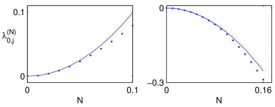
Figure 3: Eigenvalue $\lambda_{0,j}^{(N)}$ ($j=1,2$) of the operator $L_{+,\nu}^{(N)}$ as a function of ${\tilde{N}}$ for the lattice (40) and a for soliton centered at a lattice minimum (left) and at a lattice maximum (right). For ${\tilde{N}}\ll 1$, there is a good agreement between the numerically calculated eigenvalue of the discretized operator $L_{+,\nu}^{(N)}$ (dots) and the analytical approximation (54) (solid line).

4.3 Stability results

Now that we have determined when the slope and spectral conditions are satisfied, we can characterize the stability of narrow lattice solitons:

Proposition 4.2

Let ${\tilde{N}}\ll 1$, let $u_{\nu}^{(N)}$ be the solution of Eq. (16), let $p$ satisfy conditions (53) and let $V$ be given by Eq. (25). Then,

1. If $u_{\nu}^{(N)}$ is centered at a lattice maximum, then $u_{\nu}^{(N)}e^{i\nu z}$ is unstable.

2. If $u_{\nu}^{(N)}$ is centered at a lattice minimum, then $u_{\nu}^{(N)}e^{i\nu z}$ is stable in the subcritical and critical cases $p\leq 1+4/d$, and unstable in the supercritical case $p>1+4/d$.

Proof: Instability of narrow lattice solitons centered at a lattice maximum follows from a violation of the spectral condition (Proposition 4.1). For narrow lattice solitons centered at a lattice maximum the spectral condition is satisfied (Proposition 4.1) and stability is determined by the slope condition. Hence, the stability in the subcritical and critical cases and instability in the supercritical case follow from Corollary 4.2. $\Box$.

Proposition 4.2 refers only to solitons centered at a lattice minimum or maximum. In some cases (e.g., in studies of lattices with defects or surface/corner solitons [50]), lattice solitons can be centered at critical points of the lattice that are saddle points. In these cases, by Lemma 4.2, the narrow lattice solitons are unstable since the spectral condition is violated.

4.4 Instability dynamics

Proposition 4.2 specifies the conditions for which narrow lattice solitons are unstable. It does not, however, describe the instability dynamics that occur when those conditions are not met. As noted in the Introduction, in previous studies [30, 31, 40] it was observed that if the slope is negative, the solitons undergo a width instability and when the spectral condition is violated, the solitons undergo a drift instability.

In the case of narrow lattice solitons we can prove that violation of the spectral condition results in a drift instability by monitoring the dynamics of the soliton center of mass:

Lemma 4.3

Let $\langle{x_{j}}\rangle$ be the center of mass in the $x_{j}$ coordinate, i.e.,

$$\langle{x_{j}}\rangle\equiv\frac{\int x_{j}|A|^{2}d{\bf x}}{\int|A|^{2}d{\bf x}}.$$ (55)

Then,

$$\left\{\begin{array}[]{llll}\langle{x_{j}(z)}\rangle\sim\langle{x_{j}(0)}\rangle\cos(\Omega z)+\frac{\langle{\dot{x}_{j}(0)}\rangle}{\Omega}\sin(\Omega z),&&&v_{jj}>0,\\ &&&\\ \langle{x_{j}(z)}\rangle\sim\langle{x_{j}(0)}\rangle\cosh(\Omega z)+\frac{\langle{\dot{x}_{j}(0)}\rangle}{\Omega}\sinh(\Omega z),&&&v_{jj}<0,\end{array}\right.$$ (56)

where

$$\Omega=2N\sqrt{d\eta|v_{jj}|},$$ (57)

and $v_{jj}$ defined in Eq. (24).

Proof: See E.

Thus, if $v_{jj}>0$, the center of mass $\langle{x_{j}}\rangle$ oscillates around the lattice minimum. On the other hand, if $v_{jj}<0$, the center of mass moves away from the lattice maximum at an exponential rate. This shows, in particular, that a soliton centered at a saddle point is stable in the directions in which it is centered at a lattice minimum and undergoes a drift instability in the directions in which it is centered at a lattice maximum.

5 Quantitative study of stability

As noted, the lattice has a small ${\cal O}({\tilde{N}}^{2})$ effect on the slope and on the value of the perturbed near zero-eigenvalues of $L_{+,\nu}^{(N)}$. Nevertheless, this small effect changes the stability of solitons centered at a lattice maximum (which became unstable) and of solitons centered at a lattice minimum in the critical case (which become stable). As pointed out in [30, 31], when a small effect changes the stability, stability and instability needs also to be studied quantitatively.

5.1 “Mathematical” stability vs. “physical” stability

Let us first consider narrow lattice solitons centered at a lattice minimum in the critical case. In this case, according to Proposition 4.2 the solitons are stable. However, as was shown in [30, 31], satisfying the “mathematical” conditions for stability does not necessarily “prevent” the development of instabilities due to small perturbations. In order to understand how this can happen, we recall that Theorem 4.1 ensures that there is a stability region in the function space of initial conditions around the soliton profile for which the solution remains stable. However, it does not say how large this stability region is. If the stability region is very narrow, the solution is only stable under extremely small perturbations. In this case, it is “mathematically” stable but “physically unstable”, i.e., it can become unstable under perturbations present in an experimental setup. If, on the other hand, it is also stable under perturbations comparable in magnitude to perturbations in actual physical setups, one can say that it is also “physically stable”.

The distinction between “mathematical stability” and “physical stability” is only important in the critical case where, in the absence of the lattice, the slope is zero. Then, the slope (VK) condition shows that these solitons are unstable and indeed, an arbitrarily small perturbation can cause them either to undergo diffraction or to collapse. The effect of a linear lattice on narrow lattice solitons centered at a lattice minimum is to induce an ${\cal O}({\tilde{N}}^{2})$ positive correction to the power slope which causes the slope (VK) condition to be satisfied and the solitons to become stable. As demonstrated for the first time in [30, 31], the size of the stability region depends on the magnitude of the slope. This means that the transition between instability and stability is gradual rather than sharp, in the sense that as the soliton width ${\tilde{N}}$ increases from zero, the magnitude of the slope grows from zero, hence the width of the stability region grows from zero. For example, in the case of a Kronig-Penney lattice, the power slope of narrow lattice solitons is exponentially small (see Section 4.1), hence the stability region is also exponentially small. Therefore, narrow Kronig-Penney solitons are “mathematically” stable but “physically” unstable. On the other hand, in the case of a sinusoidal lattice, the stability region of the solitons is bigger, so that the sinusoidal lattice solitons can be also “physically” stable.

In order to motivate the claims stated above, we first note that by definition (31) of ${\tilde{N}}$, the slope $\partial_{\nu}\mathcal{P}_{\nu}^{(N)}$ is proportional to $\partial_{\tilde{N}}\mathcal{P}_{\nu}^{(N)}$. Thus, the slope with respect to the soliton width ${\tilde{N}}$ can be viewed as a measure for the slope with respect to the propagation constant $\nu$. Second, we recall that the soliton profile $u_{\tilde{N}}$ is an attractor for NLS solutions. Therefore, small perturbations of the initial profile essentially lead to small oscillations of the soliton width along the propagation (see below). Thus, heuristically, we can view these width oscillations as a movement along the curve $\mathcal{P}_{\nu}^{(N)}$. Such movement along the curve $P_{\nu}^{(N)}$ was demonstrated e.g. in Fig. 6 of [40]. Since the power is conserved, a large slope only allows for small changes of the soliton width (i.e., stability) while a small slope allows for larger changes of the soliton width and larger deviations from the initial state (i.e., instability). More generally, these arguments show that while the sign of the slope determines whether the solution is stable or not, the magnitude of the slope $|\partial_{\nu}\mathcal{P}_{\nu}^{(N)}|$ corresponds to the size of the stability region. Hence, if the slope $\partial_{\nu}\mathcal{P}_{\nu}^{(N)}$ is positive but small, the stability induced by the lattice is weak. Therefore, if the perturbation applied to the narrow lattice soliton is large enough, the perturbation can “overcome” the stabilization and the solution will become unstable.

A schematic illustration of the stability region in the critical case as a function of the beam power $\mathcal{P}$ and the relative width ${\tilde{N}}$ is shown in Fig. 4. The stability region is centered around the lattice soliton power $\mathcal{P}_{\nu}^{(N)}\cong\mathcal{P}_{cr}-C_{V}{\tilde{N}}^{2}$, see Eq. (38). By Eq. (44) and the above arguments, the size of the stability region depends on the propagation constant $\nu$, the period $N$ and the lattice $V({\bf x})$ only through the parameter ${\tilde{N}}$, and is ${\cal O}({\tilde{N}}^{2})$ small. Initial conditions to the left of the stability region undergo a diffraction instability whereas initial conditions to the right of the stability region undergo a blowup instability. The separatrix between the stability region and blowup region can be estimated by the critical power for collapse in homogeneous medium $\mathcal{P}_{cr}$. Indeed, while the minimal power needed for collapse depends on the beam profile, for single-hump profiles such as $u^{(N)}_{\nu}$, the minimal power needed for collapse is only slightly above $\mathcal{P}_{cr}$ [51].

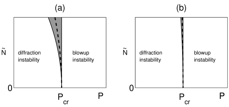
Figure 4: A schematic illustration of stability (shaded), diffraction instability and blowup instability regions as a function of the input beam width ${\tilde{N}}$ and power $\mathcal{P}$ for narrow lattice solitons centered at a minimum of (a) a sinusoidal lattice and (b) a Kronig-Penney lattice. Dashed curve is $\mathcal{P}_{\nu}^{(N)}$.

To illustrate these ideas numerically, we solve Eq. (3) for $d=d_{lat}=2$ and $p=3$, which correspond to the physical case of a $2D$ Kerr medium and ${\tilde{N}}=0.1$ (i.e., narrow lattice solitons). Since this is the critical case, the lattice should have a dominant effect on the stability (see Proposition 4.2). In order to demonstrate the difference between the stabilization by the sinusoidal lattice (40) and by the Kronig-Penney lattice (41), we perform a series of numerical simulations with the initial condition $A_{0}(x,y)=(1+\epsilon\cdot h(x,y))u_{\nu}^{(N)}$. Here $\nu=\eta=1$ and $h(x,y)$ is a random function which is uniformly distributed in $[0,1]\times[0,1]$. Hence, the perturbation increases the power of the initial condition by the factor of $\approx(1+\epsilon)$ with respect to the power of the soliton $u_{\nu}^{(N)}$. We consider narrow solitons centered at a lattice minimum, hence they are “mathematically” stable, see Table 1.

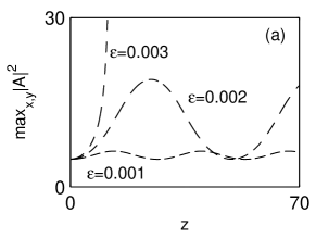
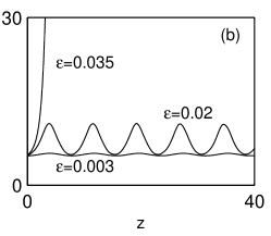
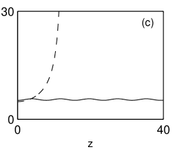
Figure 5: Maximum intensity vs. propagation distance of narrow lattice solitons ($N=0.1$) with power-increasing random perturbations for (a) Kronig-Penney lattice (41) and (b) sinusoidal lattice (40). Comparison of the dynamics for a sinusoidal lattice (solid) and Kronig-Penney lattices (dashed) is shown in (c) for $\epsilon=0.003$.

We first note that in all the simulations in this Section, the center of mass of the beam, which is initially perturbed from the lattice minimum due to the random noise, remains small and close to the lattice minimum, in accordance with Lemma 4.3.

In Fig. 5(a), we show the solution for the Kronig-Penney lattice for various values of $\epsilon>0$ (i.e., when the noise increases the beam power) for $0\leq z\leq 70$, i.e., over 140 diffraction lengths. For $\epsilon=0.001$ and $0.002$, the solution undergoes a focusing-defocusing oscillations. When the initial perturbation is further increased ($\epsilon=0.003$), the beam undergoes collapse. The abrupt change in the dynamics between $\epsilon=0.002$ and $\epsilon=0.003$ can be understood by looking at the power of the beams. For the specific noise realizations in our simulations, the power of the initial condition was slightly below the critical power $\mathcal{P}_{cr}$ for $\epsilon=0.001$ and $0.002$ and slightly above $\mathcal{P}_{cr}$ for $\epsilon=0.003$. Therefore, the beam undergoes collapse in the latter case.

While an $\epsilon=0.003$ perturbation to a Kronig-Penney lattice soliton leads to collapse, the same perturbation applied to a narrow sinusoidal lattice soliton only leads to small amplitude oscillations, see Fig. 5(b). When the perturbation is increased to $\epsilon=0.02$ the oscillations become stronger yet the solution does not collapse. Only when the perturbation is further increased to $\epsilon=0.035$ the beam collapses in a finite distance. As in Fig. 5(a), we confirmed that for $\epsilon=0.003$ and $\epsilon=0.02$ the beam power is below $P_{cr}$, while for $\epsilon=0.035$ it is above $P_{cr}$.

These simulations confirm that although both lattice solitons are “mathematically” stable, sufficiently large perturbations can still cause these stable solitons to undergo collapse . This demonstrates that collapse and stability can co-exist, see also [43, 38]. Moreover, these simulations also support the heuristic argument presented in Section 5.1 that the upper boundary of the stability region can be estimated by the critical power for collapse in homogeneous medium $P_{cr}$.

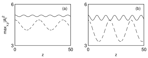
Figure 6: Maximum intensity vs. propagation distance of narrow ($N=0.1$) lattice solitons with power-decreasing random perturbations for sinusoidal (solid) and Kronig-Penney lattices (dashed) with (a) $\epsilon=-0.001$ and (b) $\epsilon=-0.003$.

In Fig. 6, we show the solutions for $\epsilon=-0.001$ and $\epsilon=-0.003$ (i.e., when the noise decreases the beam power). The comparison between the two lattices for the same value of $\epsilon$ shows that the stabilization by the sinusoidal lattice is much stronger than by a Kronig-Penney lattice. Additional simulations (data not shown) show that the difference between the stabilization by the two lattices becomes more pronounced as $N$ becomes smaller. Indeed, for a Kronig-Penney lattice, the boundaries of the lattice are located far in the soliton tail region. Thus, their presence can prevent broadening only once the narrow beam has undergone significant broadening. On the other hand, a sinusoidal lattice acts at any position in the central region of the soliton, hence, it has a much more pronounced effect.

The results shown in Figs. 5 and 6 confirm that Kronig-Penney lattice solitons are “physically unstable” (i.e., an extremely small stability region) whereas sinusoidal lattice solitons can be “physically stable” (not-so-small stability region). Indeed, a comparison between these two lattices for the same value of $\epsilon$ shows that for narrow lattice solitons, the same perturbation leads to collapse in the case of a Kronig-Penney lattice but only to small oscillations and stable behaviour in the case of a sinusoidal lattice, see Fig. 5(c) and Fig. 6.

5.2 “Mathematical” vs. “physical” instability

We now consider narrow lattice solitons centered at a lattice maximum. According to Proposition 4.2, these solitons are unstable as they violate the spectral condition. Indeed, we showed that these solitons undergo a drift instability away from the lattice maximum. Since there is no drift for $\lambda_{0,j}=0$, by continuity, the drift rate should be “small” for small negative values of $\lambda_{0}^{(N)}$. Indeed, combining Eqs. (50) and (56), one sees that for $v_{jj}<0$,

$$\langle{x_{j}(z)}\rangle\sim\langle{x_{j}(0)}\rangle\cosh(\Omega z)+\frac{\langle{\dot{x}_{j}(0)}\rangle}{\Omega}\sinh(\Omega z),\quad\Omega=2\sqrt{\frac{\eta d|\lambda_{0}^{(N)}|}{\delta}}.$$ (58)

Thus, if $-\lambda_{0}^{(N)}$ is small, the instability develops very slowly. In this case, the solitons are “mathematically” unstable but can be “physically stable”, i.e., the instability does not develop over the propagation distance of the experiment. If, on the other hand, the instability does develop over such distances, one can say that the soliton is also “physically unstable”.

In order to demonstrate the drift instability associated with violation of the spectral condition, and in particular, the importance of the magnitude of $\lambda_{0}^{(N)}$, we solve Eq. (3) with $d=1$ and $p=3$ for a sinusoidal lattice

$$V(Nx)=V_{0}\cos(2\pi Nx),$$ (59)

and also for a Kronig-Penney lattice with the unit cell that consists of a periodic array of cells of size $1/N$, where for each cell,

$$V(Nx)=\left\{\begin{array}[]{ll}V_{0},&|x|<\frac{1}{4N}\\ 0,&\frac{1}{4N}<|x|<\frac{1}{2N}.\end{array}\right.$$ (60)

We excite the instability by shifting the soliton center slightly off the lattice maximum, i.e., we use the initial condition $A_{0}(x)=u_{\nu}^{(N)}(x-\delta_{c})$. In Fig. 7 we show the center of mass of the solution for $N=0.07$, $\nu=10$, $V_{0}=2.5$ and $\delta_{c}=10^{-4}$. For these parameters, $\langle{x(0)}\rangle=\delta_{c}$ and $\langle{\dot{x}(0)}\rangle=0$ so that by Eq. (58),

$$\langle{x_{j}(z)}\rangle\sim\delta_{c}\cosh(\Omega z),\quad\quad\Omega=2\sqrt{\frac{\eta d\big{|}\lambda_{0}^{(N)}\big{|}}{\delta}}.$$ (61)

This exponential drift-rate is indeed observed in the simulation for the sinusoidal lattice soliton, see Fig. 7. This shows that while the sign of $\lambda_{0}^{(N)}$ determines whether the soliton is (“mathematically”) stable or unstable, the magnitude of $|\lambda_{0}^{(N)}|$ determines the rate of the instability dynamics.

The drift rate for the KP lattice soliton is several orders of magnitude smaller than for the sinusoidal lattice soliton. Intuitively, this is because unlike the sinusoidal lattice, the KP lattice affects the soliton profile (and hence the dynamics) only in the soliton tail region. As expected, the magnitude of $\lambda_{0}^{(N)}$ is much larger for the sinusoidal lattice soliton ($\lambda_{0}^{(N)}\cong-0.05$) than for the KP lattice soliton ($\lambda_{0}^{(N)}\cong-2\cdot 10^{-5}$). Moreover, the drift rate of the KP lattice soliton is considerably smaller than the one predicted by Eq. (61) with $\lambda_{0}^{(N)}\cong-2\cdot 10^{-5}$. This “mismatch” is not surprising, since Eq. (61) is not valid for the KP lattice, see also Section 3.1.

At a propagation distance of $z=5$, both the sinusoidal and the KP lattice solitons hardly shift from their initial location, see Fig. 8. At a propagation distance of $z=10$, however, the sinusoidal lattice soliton drifts more than one soliton width whereas the Kronig-Penney lattice soliton hardly drifts at all. In that sense, since the propagation distance in the simulations corresponds to a distance of $20$ diffraction lengths, which is longer than most devices in optics, the “mathematically unstable” KP soliton is “physically stable”.

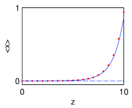
Figure 7: Center of mass of the solution of Eq. (3) with $d=1$, $p=3$ and a sinusoidal lattice (59) (solid line) and a KP lattice (60) (dashed line). The lattice parameters are $N=0.07$ and $V_{0}=2.5$; the initial shift of the soliton center is $\delta_{c}=10^{-4}$. The analytical formula (61) (red dots) is nearly indistinguishable from the numerical result.

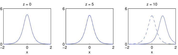
Figure 8: Beam profiles at several propagation distances for the data of Fig. 7. The beam profiles for the sinusoidal lattice (59) (solid line) and the KP lattice (60) (dashed line) at $z=0$ and $z=5$ are indistinguishable.

6 Discussion and comparison with previous studies

Most rigorous studies on stability and instability of lattice solitons are based on the Grillakis, Shatah and Strauss (GSS) theory [52, 53]. Let $u_{\nu}^{(N)}>0$, let

$$d(\nu)=\mathcal{H}+\nu\mathcal{P}=\int\left[|\nabla u_{\nu}^{(N)}|^{2}+\left(V(N{\bf x}_{lat})+\nu\right)\left(u_{\nu}^{(N)}\right)^{2}-\frac{2}{p+1}\left(u_{\nu}^{(N)}\right)^{p+1}\right]d{\bf x},$$

let $p(d^{\prime\prime})=1$ if $d^{\prime\prime}>0$ and $p(d^{\prime\prime})=0$ if $d^{\prime\prime}<0$, and let $n_{-}(L_{+,\nu}^{(N)})$ be the number of negative eigenvalues of the operator $L_{+,\nu}^{(N)}$. Then, $u_{\nu}^{(N)}e^{i\nu z}$ is orbitally stable if $n_{-}(L_{+,\nu}^{(N)})=p(d^{\prime\prime})$, and orbitally unstable if $n_{-}(L_{+,\nu}^{(N)})-p(d^{\prime\prime})$ is odd [52, 53]. For example, stability of lattice solitons was studied in [54, 55, 56, 35] using the GSS theory. In addition, after this paper was submitted, we found out that the GSS theory was applied to narrow lattice solitons in the critical case by Lin and Wei [34].

Since $d^{\prime}(\nu)=\int\left(u_{\nu}^{(N)}\right)^{2}d{\bf x}$, the sign of $d^{\prime\prime}$ is the same as the sign of the power slope. Hence, in the GSS theory stability and instability depend on a combination of the slope condition and a spectral condition: If both the slope condition and the spectral condition are satisfied, the soliton is stable, whereas if either the slope condition is satisfied and $n_{-}(L_{+,\nu}^{(N)})$ is even, or if the slope condition is violated and $n_{-}(L_{+,\nu}^{(N)})$ is odd, the soliton is unstable. There are two cases not covered by the GSS theory: When the slope condition is satisfied and $n_{-}(L_{+,\nu}^{(N)})$ is odd, and when the slope condition is violated and $n_{-}(L_{+,\nu}^{(N)})$ is even. As Theorem 4.1 shows, in both cases the solitons are unstable. Hence, there is a “decoupling” of the slope and spectral conditions, in the sense that both are needed for stability, and violation of either of them would lead to instability.

In [30, 31, 40] it was observed numerically that violation of the slope condition leads to a width instability, whereas violation of the spectral condition leads to a drift instability. Unlike these studies, in this study we prove that violation of the spectral condition leads to a drift instability. Moreover, we show that a drift instability occurs in any direction $x_{j}$ for which the corresponding eigenvalue $\lambda_{0,j}^{(N)}$ is negative, and that the drift rate is determined by the magnitude of $\lambda_{0,j}^{(N)}$.  This further shows that violation of the spectral condition leads to an instability, regardless of the slope condition and of whether $n_{-}(L_{+,\nu}^{(N)})$ is even or odd.

In previous studies it was also observed that in the subcritical case, lattice solitons centered at a lattice minimum of all widths are stable. In the critical case, it was shown that lattice solitons are stable only if they are narrower than a few lattice periods, see e.g., [17, 19]. These results are in agreement with Table 1 in the subcritical and critical cases, and imply that our analytical results are valid beyond the regime of narrow lattice solitons. In [20, 21] it was also shown that in the supercritical case, the lattice can stabilize sufficiently wide lattice solitons centered at a lattice minimum but cannot stabilize narrow lattice solitons, in agreement with our results. Note, however, that unlike most previous works, our results are valid for any dimension $d$, lattice dimension $d_{lat}$ and nonlinearity exponent $p$.

Another difference from previous studies on linear lattices is that we introduce a quantitative approach to the notions of stability and instability. Thus, we show that the strength of radial stabilization depends on the magnitude of the slope. Hence, in the critical case, the stability of the soliton is “mathematical” but not “physical”. Similarly, we show that the strength of the transverse instability depends on the value of the perturbed zero eigenvalue $\lambda_{0}^{(N)}$. Hence, for narrow solitons centered at a lattice maximum, the instability is “mathematical” but not necessarily “physical”. In such cases, the stabilization/destabilization of narrow lattice solitons is highly sensitive to the lattice details. This sensitivity becomes smaller as the soliton width increases, and is of considerably less importance for ${\cal O}(1)$ solitons, which is probably why this feature was not observed in previous studies.

Appendix A Proof of Lemma 3.1

The approach used here is similar to [30, 38]. Substituting the expansion (22) in Eq. (18) gives

$$\nabla^{2}u_{\tilde{N}}+u_{\tilde{N}}^{p}-\Big{(}1+{\tilde{N}}^{2}\tilde{V}_{2}(\tilde{\bf x}_{lat})\Big{)}u_{\tilde{N}}+{\cal O}({\tilde{N}}^{4})=0.$$

Let $u_{\tilde{N}}(\tilde{\bf x})$ be given by Eq. (20). Then, the equation for $g$ is

$$\nabla^{2}g(\tilde{\bf x})+p{\cal U}^{p-1}g-\nu g=\tilde{V}_{2}(\tilde{\bf x}_{lat}){\cal U}(|\tilde{\bf x}|).$$

Therefore,

$$g(\tilde{\bf x})=-L_{+}^{-1}\big{[}\tilde{V}_{2}(\tilde{\bf x}_{lat}){\cal U}(|\tilde{\bf x}|)\big{]}.$$ (62)

Appendix B Proof of Lemma 4.1

By Eq. (27), the power of the rescaled lattice soliton $\mathcal{P}_{\tilde{N}}=\int\big{(}u_{\tilde{N}}(\tilde{\bf x})\big{)}^{2}d\tilde{\bf x}$ is given by

$$\mathcal{P}_{\tilde{N}} = \mathcal{P}_{\nu=1}-2{\tilde{N}}^{2}\int{\cal U}(\tilde{r})L_{+}^{-1}\big{[}\tilde{V}_{2}(\tilde{\bf x}_{lat}){\cal U}\big{]}d\tilde{\bf x}+{\cal O}({\tilde{N}}^{4})$$ (63)

$$= \mathcal{P}_{\nu=1}-2{\tilde{N}}^{2}\int\tilde{V}_{2}(\tilde{\bf x}_{lat}){\cal U}(\tilde{r})L_{+}^{-1}\left[{\cal U}\right]d\tilde{\bf x}+{\cal O}({\tilde{N}}^{4}),$$

where $\mathcal{P}_{\nu=1}=\int{\cal U}^{2}(\tilde{r})d\tilde{\bf x}$ and $\tilde{r}=|\tilde{\bf x}|$. In order to proceed, we prove the following Lemma:

Lemma B.1

Let ${\cal U}_{\eta}$ be the solution of Eq. (30) and let $L_{+,\eta}$ be given by Eq. (45). Then, $L_{+,\eta}^{-1}{\cal U}_{\eta}=-\partial_{\eta}{\cal U}_{\eta}$.

Proof: Differentiating Eq. (30) with respect to $\eta$ gives

$$\partial_{\eta}\ (\nabla^{2}{\cal U}_{\eta})+\partial_{\eta}\ {\cal U}_{\eta}^{p}-\partial_{\eta}\ (\eta{\cal U}_{\eta})=\nabla^{2}\ (\partial_{\eta}{\cal U}_{\eta})+p{\cal U}_{\eta}^{p-1}\ (\partial_{\eta}{\cal U}_{\eta})-{\cal U}_{\eta}-\eta\partial_{\eta}{\cal U}_{\eta}=$$

$$=-L_{+}\partial_{\eta}{\cal U}_{\eta}-{\cal U}_{\eta}=0.\quad\Box.$$

Since ${\cal U}_{\eta}(\tilde{r})=\eta^{\frac{1}{p-1}}{\cal U}(\sqrt{\eta}\tilde{r})$, then

$$\partial_{\eta}{\cal U}_{\eta}=\frac{1}{p-1}\eta^{\frac{1}{p-1}-1}{\cal U}+\eta^{\frac{1}{p-1}}\left(\frac{1}{2}\eta^{-\frac{1}{2}}\tilde{r}\right){\cal U}_{\tilde{r}}.$$

Therefore, $L_{+}^{-1}{\cal U}=L_{+}^{-1}{\cal U}_{\eta=1}=-(\partial_{\eta}{\cal U}_{\eta})_{\eta=1}=-\frac{1}{p-1}{\cal U}-\frac{1}{2}\tilde{r}{\cal U}_{\tilde{r}}$. Substituting in Eq. (63) gives

$$\mathcal{P}_{\tilde{N}} = \mathcal{P}_{\nu=1}+2{\tilde{N}}^{2}\int\tilde{V}_{2}(\tilde{\bf x}_{lat}){\cal U}\left(\frac{{\cal U}}{p-1}+\tilde{r}\frac{{\cal U}_{\tilde{r}}}{2}\right)d\tilde{\bf x}+{\cal O}({\tilde{N}}^{4}).$$ (64)

Since $\tilde{V}_{2}$ is given by Eq. (24), Eq. (64) can be written as

$$\mathcal{P}_{\tilde{N}} = \mathcal{P}_{\nu=1}-C_{V}{\tilde{N}}^{2}\sum_{j=1}^{d_{lat}}v_{jj}+{\cal O}({\tilde{N}}^{4}),$$

where $C_{V}$ is given by

$$C_{V} = -\int\tilde{x}_{j}^{2}\left(\frac{2{\cal U}^{2}}{p-1}+\tilde{r}{\cal U}{\cal U}_{\tilde{r}}\right)d\tilde{\bf x}.$$ (65)

To bring $C_{V}$ to the form (39), we note that

$$\nabla\cdot\left(b(\tilde{r})\tilde{\bf x}\right)=\frac{1}{\tilde{r}^{d-1}}\frac{\partial}{\partial\tilde{r}}\left(\tilde{r}^{d}b(\tilde{r})\right)=\frac{1}{\tilde{r}^{d-1}}\left(d\tilde{r}^{d-1}b+\tilde{r}^{d}b^{\prime}\right)=db+\tilde{r}b^{\prime}.$$

Substituting $b(\tilde{r})=\tilde{r}^{\frac{4}{p-1}-d}{\cal U}^{2}(\tilde{r})$ shows that

$$\nabla\cdot\left(\tilde{r}^{\frac{4}{p-1}-d}{\cal U}^{2}(\tilde{r}){\bf x}\right) = d\tilde{r}^{\frac{4}{p-1}-d}{\cal U}^{2}+\left(\frac{4}{p-1}-d\right)\tilde{r}^{\frac{4}{p-1}-d}{\cal U}^{2}+2\tilde{r}^{\frac{4}{p-1}-d+1}{\cal U}{\cal U}^{\prime}$$

$$= 2\tilde{r}^{\frac{4}{p-1}-d}\left(\frac{2{\cal U}^{2}}{p-1}+\tilde{r}{\cal U}{\cal U}_{\tilde{r}}\right).$$

Thus, we can rewrite Eq. (65) as

$$C_{V} = -\frac{1}{2}\int\frac{\tilde{x}_{j}^{2}}{\tilde{r}^{\frac{4}{p-1}-d}}\nabla\cdot\left(\tilde{r}^{\frac{4}{p-1}-d}{\cal U}^{2}\tilde{\bf x}\right)d\tilde{\bf x}$$

$$= \frac{1}{2}\int r^{\frac{4}{p-1}-d}{\cal U}^{2}\tilde{\bf x}\cdot\nabla\left(\frac{\tilde{x}_{j}^{2}}{\tilde{r}^{\frac{4}{p-1}-d}}\right)d\tilde{\bf x}$$

$$= \frac{1}{2}\int r^{\frac{4}{p-1}-d}{\cal U}^{2}\tilde{\bf x}\cdot\left(\frac{2\tilde{x}_{j}\hat{\bf e}_{\tilde{x}_{j}}}{\tilde{r}^{\frac{4}{p-1}-d}}-\left(\frac{4}{p-1}-d\right)\frac{\tilde{x}_{j}^{2}\hat{\bf e}_{\tilde{r}}}{\tilde{r}^{\frac{4}{p-1}-d+1}}\right)d\tilde{\bf x}$$

$$= \frac{1}{2}\int{\cal U}^{2}\left(2\tilde{x}^{2}_{j}-\left(\frac{4}{p-1}-d\right)\tilde{x}_{j}^{2}\right)d\tilde{\bf x}=\frac{1}{2d}\int\tilde{r}^{2}{\cal U}^{2}\left(2-\frac{4}{p-1}+d\right)d\tilde{\bf x}.$$

Finally, by the dilation transformation (17),

$$\mathcal{P}_{\nu}^{(N)} \equiv \int\left(u_{\nu}^{(N)}({\bf x})\right)^{2}d{\bf x}=\eta^{\frac{2}{p-1}}\int\left(u_{\tilde{N}}(\tilde{\bf x})\right)^{2}d{\bf x}=\eta^{\frac{4-d(p-1)}{2(p-1)}}\mathcal{P}_{\tilde{N}}.$$

Appendix C Proof of Lemma 4.2

Consider the eigenvalue problem

$$L_{+,\nu}^{(N)}f^{(N)}_{\nu,j}({\bf x})=\lambda_{0,j}^{(N)}f^{(N)}_{\nu,j}.$$ (67)

Multiplying Eq. (67) by $f^{(N)}_{\nu,j}$ and integrating gives

$$\int f^{(N)}_{\nu,j}L_{+,\nu}^{(N)}f^{(N)}_{\nu,j}d{\bf x}=\lambda_{0,j}^{(N)}\int\left(f^{(N)}_{\nu,j}\right)^{2}d{\bf x}.$$ (68)

We recall that in the absence of a lattice, the operator $L_{+,\nu}^{(N)}$ reduces to $L_{+,\nu}$, see Eq. (45), which has $d$ zero eigenvalues $\lambda_{0,j}=0$, with the corresponding eigenfunctions $\frac{\partial{\cal U}_{\nu}}{\partial x_{j}}$ for $j=1,\dots,d$, see Eq. (46). By Eq. (29), in the presence of the lattice, $u_{\nu}^{(N)}={\cal U}_{\eta}+\eta^{\frac{1}{p-1}}{\cal O}({\tilde{N}}^{2})$. Similarly, by Eq. (19), Eq. (22) and Eq. (24), we can expand the potential as

$$V(N{\bf x}_{lat})=V({\tilde{N}}\tilde{\bf x}_{lat})=V(0)+\eta\tilde{V}({\tilde{N}}\tilde{\bf x}_{lat})=V(0)+\eta\left({\tilde{N}}^{2}\tilde{V}_{2}(\tilde{\bf x}_{lat})+{\cal O}({\tilde{N}}^{4})\right)$$ (69)

$$=V(0)+N^{2}\sum_{j=1}^{d_{lat}}v_{jj}\tilde{x}_{j}^{2}+\eta\cdot{\cal O}({\tilde{N}}^{4})=V(0)+\eta N^{2}\sum_{j=1}^{d_{lat}}v_{jj}x^{2}_{j}+\eta\cdot{\cal O}({\tilde{N}}^{4}).$$

Consequently, the operator $L^{(N)}_{+,\nu}$ can be expanded as

$$L_{+,\nu}^{(N)} = -\nabla^{2}-p\left(u_{\nu}^{(N)}\right)^{p-1}+\nu+V(N{\bf x}_{lat})$$

$$= -\nabla^{2}-p\left({\cal U}_{\eta}+\eta^{\frac{1}{p-1}}{\cal O}({\tilde{N}}^{2})\right)^{p-1}+\nu+V(0)+{\cal O}(N^{2})$$

$$= -\nabla^{2}-p{\cal U}_{\eta}^{p-1}+\eta+{\cal O}(N^{2})=L_{+,\eta}+{\cal O}(N^{2}).$$

Therefore, we expand

$$f^{(N)}_{\nu,j}({\bf x})=\frac{\partial{\cal U}_{\eta}}{\partial x_{j}}\left(1+{\cal O}(N^{2})\right),\quad\quad\lambda_{0,j}^{(N)}=\delta_{j}N^{2}+{\cal O}(N^{4}).$$ (71)

By Eqs. (29) and (71), we can also rewrite the eigenfunction $f^{(N)}_{\nu,j}$ as

$$f^{(N)}_{\nu,j}({\bf x})=\frac{\partial u_{\nu}^{(N)}}{\partial x_{j}}\left(1+{\cal O}(N^{2})\right).$$ (72)

We now use the approximations (71) and (72) in order to evaluate the terms in Eq (68). By Eq. (71), the right-hand-side of Eq. (68) is equal to

$$\lambda_{0,j}^{(N)}\int\left(f_{\nu}^{(N)}\right)^{2}d{\bf x} = \left(N^{2}\delta_{j}+{\cal O}(N^{4})\right)\left(\int\left(\frac{\partial{\cal U}_{\eta}}{\partial x_{j}}\right)^{2}d{\bf x}+{\cal O}(N^{2})\right)$$ (73)

$$= N^{2}\delta_{j}\int\left(\frac{\partial{\cal U}_{\eta}}{\partial x_{j}}\right)^{2}d{\bf x}+{\cal O}(N^{4}).$$

By Eq. (72) the left-hand-side of Eq. (68), approximation (72) is equal to

$$\int f^{(N)}_{\nu,j}L_{+,\nu}^{(N)}f^{(N)}_{\nu,j}d{\bf x}=\int\frac{\partial u_{\nu}^{(N)}}{\partial x_{j}}L_{+,\nu}^{(N)}\frac{\partial u_{\nu}^{(N)}}{\partial x_{j}}d{\bf x}+{\cal O}(N^{4}),$$ (74)

where the error term is ${\cal O}(N^{4})$ due to the properties of the Rayleigh quotient, see e.g., [58].

The integral term on the right-hand-side of Eq. (74) is equal to

$$\int\frac{\partial u_{\nu}^{(N)}}{\partial x_{j}}L_{+,\nu}^{(N)}\frac{\partial u_{\nu}^{(N)}}{\partial x_{j}}d{\bf x}=\frac{1}{2}\int\left(u_{\nu}^{(N)}\right)^{2}\frac{\partial^{2}}{\partial x^{2}_{j}}V(N{\bf x}_{lat})d{\bf x}.$$ (75)

Indeed, differentiating Eq. (16) with respect to $x_{j}$ gives

$$L_{+,\nu}^{(N)}\frac{\partial u_{\nu}^{(N)}}{\partial x_{j}}=-\left(\frac{\partial V(N{\bf x}_{lat})}{\partial x_{j}}\right)u_{\nu}^{(N)}.$$ (76)

Multiplying Eq. (76) by $\frac{\partial}{\partial x_{j}}u_{\nu}^{(N)}$, integrating over ${\bf x}$ and integrating by parts gives Eq. (75). Using Eq. (69), the right-hand-side of Eq. (75) is given by

$$\frac{1}{2}\int\left(u_{\nu}^{(N)}\right)^{2}\frac{\partial^{2}}{\partial x^{2}_{j}}V(N{\bf x}_{lat})d{\bf x}=\eta N^{2}v_{jj}\int{\cal U}_{\eta}^{2}d{\bf x}+{\cal O}(N^{4}).$$ (77)

Comparing the approximation (73) for the left-hand-side of Eq. (68) with the approximation (77) for the right-hand-side of Eq. (68) shows that

$$\delta_{j}\int\left(\frac{\partial{\cal U}_{\eta}}{\partial x_{j}}\right)^{2}=\eta v_{jj}\int{\cal U}_{\eta}^{2}.$$ (78)

Hence,

$$\delta_{j}=\eta v_{jj}\frac{\int{\cal U}_{\eta}^{2}}{\int\left(\frac{\partial{\cal U}_{\eta}}{\partial x_{j}}\right)^{2}}=dv_{jj}\frac{\int{\cal U}^{2}}{\int{{\cal U}^{\prime}}^{2}}.$$ (79)

Similar results were obtained in [34] for a soliton centered at a general non-degenerate critical point of the lattice (i.e., without assuming that the critical point is symmetric with respect to ${\bf x}_{lat}^{(0)}$).

By the Pohozaev identities for Eq. (21) (see [59], pp. 76), $\frac{\int{\cal U}^{2}}{\int{{\cal U}^{\prime}}^{2}}=\frac{p(2-d)+2+d}{d(p-1)}\equiv\frac{\delta}{d}$. Therefore, we get that

$$\delta_{j}=\delta v_{jj}.$$ (80)

Appendix D Computing small eigenvalues of a very large matrix

When $d\geq 2$, the discretized operator $L_{+}^{(N)}$ is represented by an extremely large matrix. Hence, straightforward application of standard numerical routines (such as Matlab’s eig/eigs) usually either fails to give accurate results or does not converge.

In order to overcome this numerical problem, we used a more efficient and robust numerical method based on the Arnoldi algorithm (performed by ARPACK [60], which is available in Matlab through the function eigs). Essentially, we compute the largest-magnitude eigenvalues of the inverse matrix $A^{-1}$ which correspond to the smallest eigenvalues of the matrix $A$.

We compute the $LU$ factorization of $A$ with complete pivoting. Then, we shift the values on the main diagonal of $U$ by a small value in order to avoid numerical errors that might result from singularity of the matrix during the computation of $A^{-1}$. Then, in order to avoid working with the explicit from of the inverse matrix $A^{-1}$ which is dense, we compute $A^{-1}$ implicitly through the subfunction ${\tt LUPinv}$ and apply it to the function ${\tt eigs}$. This way, we exploit the sparsity of the $LU$ factorized matrices $U$ and $L$. The function ${\tt eigs}$ then computes the desired number of eigenvalues of largest magnitude.

The following code was given to us by Prof. S. Toledo:

function [V,d] = ev_calculation(A,ev_number,eps)

[m n] = size(A); normA = norm(A,1);

[L,U,P,Q] = lu(A,1.0);

for j=1:n

if (abs(U(j,j)) < eps*normA)

U(j,j) = eps*normA;

end

end

h = @LUPinv;

opts.issym = true;

opts.isreal = true;

opts.tol = eps;

[V,D] = eigs(h,n,ev_number,’LM’,opts);

function Y = LUPinv(X)

Y1 = P*X;

Y2 = L $\setminus$ Y1;

Y3 = U $\setminus$ Y2;

Y = Q*Y3;

end

end

Appendix E Proof of Lemma 4.3

Multiplying Eq. (3) by $A^{*}$ and subtracting the conjugate equation gives

$$\frac{d}{dz}|A|^{2}=iA^{*}\nabla^{2}A+c.c.,$$

where c.c. stands for complex conjugate. Multiplying by ${\bf x}$ and integrating over ${\bf x}$ gives

$$\frac{d}{dz}\int{\bf x}|A|^{2} = \int i{\bf x}A^{*}\nabla^{2}A+c.c.=-i\int\nabla A(dA^{*}+{\bf x}\cdot\nabla A^{*})+c.c.$$ (81)

$$= 2d\ Im\int A^{*}\nabla A.$$

Differentiating Eq. (81) yields

$$\frac{d^{2}}{dz^{2}}\int{\bf x}|A|^{2} = 2d\ Im\int(A_{z}^{*}\nabla A+A^{*}\nabla A_{z})$$

$$= 2d\ Im\int(A_{z}^{*}\nabla A-A_{z}\nabla A^{*})=4d\ Im\int A_{z}^{*}\nabla A$$

$$= -4d\ Re\int\left(\nabla^{2}A^{*}+|A|^{p-1}A^{*}-V(Nx)A^{*}\right)\nabla A.$$

The first two terms vanish since they are complete derivatives. Therefore,

$$\frac{d^{2}}{dz^{2}}\int{\bf x}|A|^{2} = 4d\ Re\int V(Nx)A^{*}\nabla A$$ (82)

$$= 2d\int V(N{\bf x}_{lat})\nabla|A|^{2}=-2d\int|A|^{2}\nabla V(N{\bf x}_{lat}).$$

Finally, by Eq. (25),

$$\frac{d^{2}}{dz^{2}}\int x_{j}|A|^{2}=-4N^{2}d\eta v_{jj}\int x_{j}|A|^{2}+{\cal O}(N^{4}).$$ (83)

References

References

- [1] M. I. Weinstein. The nonlinear Schrödinger equation: singularity formation, stability and dispersion. Amer. Math. Soc., Providence, R.I., 1989.
- [2] M.I. Weinstein. Nonlinear Schrödinger equations and sharp interpolation estimates. Comm. Math. Phys., 87:567–576, 1982/3.
- [3] D.N. Christodoulides, F. Lederer, and Y. Silberberg. Discretizing light behaviour in linear and nonlinear waveguide lattices. Nature, 424:817–823, 2003.
- [4] J.J. Joannopoulos, R.D. Meade, and J.N. Winn. Photonic crystals - molding the flow of light. Princeton University Press, 1995.
- [5] E. Ostrovskaya and Y. Kivshar. Photonic crystals for matter waves: Bose-Einstein condenstaes in optical lattices. Opt. Exp., 12:19, 2004.
- [6] J.W. Fleischer, G. Bartal, O. Cohen, T. Schwartz, O. Manela, B. Freedman, M. Segev, H. Buljan, and N.K. Efremidis. Spatial photonics in nonlinear waveguide arrays. Opt. Exp., 13:1780–1796, 2005.
- [7] A.B. Aceves, C. De Angelis, T. Peschel, R. Muschall, F. Lederer, S. Trillo, and S. Wabnitz. Discrete self-trapping, soliton interactions, and beam steering in nonlinear waveguide arrays. Phys. Rev. E, 53:1172–1189, 1996.
- [8] A.B. Aceves, G.G. Luther, C. De Angelis, A.M. Rubenchik, and S.K. Turitsyn. Energy localization in nonlinear fiber arrays: collapse-effect compressor. Phys. Rev. Lett., 75:73–6, 1995.
- [9] F.Kh. Abdullaev, A. Gammal, A.M. Kamchatnov, and L. Tomio. Dynamics of bright solitons in a Bose-Einstein condensate. Int. J. of Mod. Phys. B, 19:3415–3473, 2005.
- [10] V.A. Brazhnyi and V. V. Konotop. Theory of nonlinear matter waves in optical lattices. Mod. Phys. Lett. B, 18:627, 2004.
- [11] Y.-G. Oh. Stability of semiclassical bound states of nonlinear Schrödinger equations with potentials. Comm. Math. Phys., 121:11–33, 1989.
- [12] H.A. Rose and M.I. Weinstein. On the bound states of the nonlinear Schrödinger equation with a linear potential. Physica D, 30:207–218, 1988.
- [13] D.N. Christodoulides and R.I. Joseph. Discrete self-focusing in nonlinear arrays of coupled waveguides. Opt. Lett., 13:794–796, 1988.
- [14] P.J.Y. Louis, E.A. Ostrovskaya, C.M. Savage, and Y.S. Kivshar. Bose-Einstein condensates in optical lattices: Band-gap structure and solitons. Phys. Rev. A, 67:013602, 2003.
- [15] N.K. Efremidis and D.N. Christodoulides. Lattice solitons in Bose-Einstein condensates. Phys. Rev. A, 67:063608, 2003.
- [16] D.E. Pelinovsky, A.A. Sukhorukov, and Y. Kivshar. Bifurcations and stability of gap solitons in periodic potentials. Phys. Rev. E, 70:036618, 2004.
- [17] N.K. Efremidis, J. Hudock, D.N. Christodoulides, J.W. Fleischer, O. Cohen, and M. Segev. Two-dimensional optical lattice solitons. Phys. Rev. Lett., 91:213906, 2003.
- [18] J. Yang and Z.H. Musslimani. Fundamental and vortex solitons in a two-dimensional optical lattice. Opt. Lett., 21:2094–2096, 2003.
- [19] Z.H. Musslimani and J. Yang. Self trapping of light in a two dimensional photonic lattice. J. Opt. Soc. Am. B, 21:973–981, 2004.
- [20] D. Mihalache, D. Mazilu, F. Lederer, B.A. Malomed, L.-C. Crasovan, Y.V. Kartashov, and L. Torner. Stable three-dimensional solitons in attractive bose-einstein condensates loaded in an optical lattice. Phys. Rev. A, 72:021601, 2005.
- [21] D. Mihalache, D. Mazilu, F. Lederer, B.A. Malomed, L.-C. Crasovan, Y.V. Kartashov, and L. Torner. Stable three-dimensional spatiotemporal solitons in a two-dimensional photonic lattice. Phys. Rev. E, 70:055603(R), 2004.
- [22] H.B. Eisenberg, Y. Silberberg, R. Morandotti, A.R. Boyd, and J.S. Aitchison. Discrete spatial optical solitons in waveguide arrays. Phys. Rev. Lett., 81:3383–3386, 1998.
- [23] N.K. Efremidis, D.N. Christodoulides, S. Sears, J.W. Fleischer, and M. Segev. Discrete solitons in photorefractive optically-induced photonic lattices. Phys. Rev. E, 66:046602, October 2002.
- [24] J.W. Fleischer, T. Carmon, M. Segev, N.K. Efremidis, and D.N. Christodoulides. Observation of discrete solitons in optically-induced real-time waveguide arrays. Phys. Rev. Lett., 90:023902, 2003.
- [25] J.W. Fleischer, M. Segev, N.K. Efremidis, and D.N. Christodoulides. Observation of two-dimensional discrete solitons in optically-induced nonlinear photonic lattices. Nature, 422:147, 2003.
- [26] D. Neshev, E. Ostrovskaya, Y. Kivshar, and W. Krolikowski. spatial solitons in optically induced gratings. Opt. Lett., 28:710, 2003.
- [27] T. Pertsch, U. Peschel, F. Lederer, J. Burghoff, M. Will, S. Nolte, and A. Tünnermann. Discrete diffraction in two-dimensional arrays of coupled waveguides in silica. Opt. Lett., 29:468–470, 2004.
- [28] B.B. Baizakov, B.A. Malomed, and M. Salerno. Multidimensional solitons in a low-dimensional periodic potential. Phys. Rev. A, 70:053613, 2004.
- [29] G. L. Alfimov, V. V. Konotop, and P. Pacciani. Stationary localized modes for the quintic nonlinear schrödinger equation with a periodic potential. Phys. Rev. A, 75:023624, 2007.
- [30] G. Fibich, Y. Sivan, and M.I. Weinstein. Bound states of NLS equations with a periodic nonlinear microstructure. Physica D, 217:31–57, 2006.
- [31] Y. Sivan, G. Fibich, and M.I. Weinstein. Waves in nonlinear lattices - ultrashort optical pulses and bose-einstein condensates. Phys. Rev. Lett., 97:193902, 2006.
- [32] D. Cheskis, S. Bar-Ad, R. Morandotti, J.S. Aitchison, H.S. Heisenberg, Y. Silberberg, and D. Ross. Strong spatiotemporal localization in a silica nonlinear waveguide array. Phys. Rev. Lett., 91:223901, 2003.
- [33] T. Pertsch, U. Peschel, J. Kobelke, K. Schuster, H. Bartelt, S. Nolte, A. Tünnermann, and F. Lederer. Nonlinearity and disorder in fiber arrays. Phys. Rev. Lett., 93:053901–1–4, 2004.
- [34] T.C. Lin and J. Wei. Orbital stability of bound states of semi-classical nonlinear schrödinger equation with critical nonlinearity. SIAM J. Math. Anal., To appear.
- [35] R. Fukuizumi. Stability of standing waves for nonlinear schrödinger equations with critical power nonlinearities and potentials. Adv. Differential Equations, 10:259, 2005.
- [36] N.G. Vakhitov and A.A. Kolokolov. Stationary solutions of the wave equation in a medium with nonlinearity saturation. Izv. Vyssh. Uchebn. Zaved. Radiofiz., 16:1020, 1973.
- [37] M.I. Weinstein. Lyapunov stability of ground states of nonlinear dispersive evolution equations. Comm. Pure Appl. Math., 39:51–68, 1986.
- [38] G. Fibich and X.P. Wang. Stability of solitary waves for nonlinear schrödinger equations with inhomogeneous nonlinearities. Physica D, 175:96–108, 2003.
- [39] M.G. Grillakis. Linearized instability for nonlinear Schrödinger and Klein-Gordon equations. Comm. Pure Appl. Math., 41:747–774, 1988.
- [40] S. Le-Coz, R. Fukuizumi, G. Fibich, B. Ksherim, and Y. Sivan. Instability of bound states for a nonlinear schrödinger equation with a dirac potential. Physica D, To appear.
- [41] A. Trombettoni and A. Smerzi. Discrete Solitons and Breathers with Dilute Bose-Einstein Condensates. Phys. Rev. Lett., 86:2353–2356, 2001.
- [42] L.D. Carr, K.W. Mahmud, and W.P. Reinhardt. Tunable tunneling: An application of stationary states of Bose-Einstein condensates in traps of finite depth. Phys. Rev. A, 64:033603, 2001.
- [43] G. Fibich and F. Merle. Self-focusing on bounded domains. Physica D, 155:132–158, 2001.
- [44] B.A. Malomed, Z.H. Wang, P.L. Chu, and G.D. Peng. Multichannel switchable system of spatial solitons. J. Opt. Soc. Am. B, 16:1197, 1999.
- [45] E.H. Lieb, R. Seiringer, and J. Yngvason. One-dimensional bosons in three-dimensional traps. Phys. Rev. Lett., 91:150401, 2003.
- [46] W. Bao, Y. Ge, D. Jaksch, P.A. Markowich, and R.M. Weishäupl. Convergence rate of dimension reduction in Bose-Einstein condensates. Comput. Phys. Comm, 177:832, 2007.
- [47] M. Grossi. On the number of single peaked solitos of the nonlinear schrödinger equations. Ann. I.H. Poincare-AN, 19:261, 2002.
- [48] A. Smerzi and A. Trombettoni. Discrete nonlinear dynamics of weakly coupled Bose-Einstein condensates. Chaos, 13:766–776, 2003.
- [49] M.I. Weinstein. Modulational stability of ground states of nonlinear Schrödinger equations. SIAM J. Math. Anal., 16:472–491, 1985.
- [50] M.J. Ablowitz, B. Ilan, E. Schonbrun, and R. Piestun. Solitons in two-dimensional lattices possessing defects, dislocations, and quasicrystal structures. Phys. Rev. E, 74:035601(R), 2006.
- [51] G. Fibich and A.L. Gaeta. Critical power for self-focusing in bulk media and in hollow waveguides. Opt. Lett., 25:335, 2000.
- [52] M.G. Grillakis, J. Shatah, and W.A. Strauss. Stability theory of solitary waves in the presence of symmetry i. J. Funct. Anal., 74(1):160–197, 1987.
- [53] M.G. Grillakis, J. Shatah, and W.A. Strauss. Stability theory of solitary waves in the presence of symmetry ii. J. Funct. Anal., 94(1):308–348, 1990.
- [54] L. Bergé, T.J. Alexander, and Y.S. Kivshar. Stability criterion for attractive Bose-Einstein condensates. Phys. Rev. A, 62:023607, 2000.
- [55] R. Fukuizumi. Stability and instability of standing waves for the nonlinear schrödinger equation with harmonic potential. Discrete Contin. Dynam. Systems, 7:525–544, 2001.
- [56] R. Fukuizumi and M. Ohta. Instability of standing waves for nonlinear schrödinger equations with potentials. Diff. and Int. Eqs., 16:691–706, 2003.
- [57] Y. Sivan, G. Fibich, and B. Ilan. Submitted to Phys. Rev. Lett.
- [58] L.N. Trefethen and D. Bau. Numerical linear algebra. SIAM, Philadelphia, PA, 1997.
- [59] C. Sulem and P.L. Sulem. The Nonlinear Schrödinger Equation. Springer, New York, NY, 1999.
- [60] R. B. Lehoucq, D. C. Sorensen, and C. Yang. ARPACK User’s Guide: Solution of Large-Scale Eigenvalue Problems with Implicitly Restarted Arnoldi Methods. SIAM, Philadelphia, PA, 1998.