A Tight Lower Bound to the Outage Probability of Discrete-Input Block-Fading Channels

Abstract

In this correspondence, we propose a tight lower bound to the outage probability of discrete-input Nakagami-$m$ block-fading channels. The approach permits an efficient method for numerical evaluation of the bound, providing an additional tool for system design. The optimal rate-diversity trade-off for the Nakagami-$m$ block-fading channel is also derived and a tight upper bound is obtained for the optimal coding gain constant.

I Introduction

The block-fading channel [1, 2] is a useful channel model for a class of slowly-varying wireless communication channels. The model is particularly relevant for delay-constraint applications where channel usage is restricted to only include a finite number of distinct channel blocks, each subject to independent flat fading. Frequency-hopping schemes as encountered in the Global System for Mobile Communication (GSM) and the Enhanced Data GSM Environment (EDGE), respectively, as well as orthogonal frequency division multiplexing (OFDM) as encountered in more recently proposed wireless communication systems standards can conveniently be modeled as block-fading channels. The simplified model is mathematically tractable, while still capturing the essential features of the practical slowly-varying fading channels.

In a block-fading channel, a codeword spans a finite number of $B$ independent fading blocks. As the channel relies on particular realizations of the finite number of independent fading coefficients, the channel is non-ergodic and therefore not information stable [3, 4]. It follows that the Shannon capacity of this channel is zero since there is an irreducible probability that a given transmission rate $R$ is not supported by a particular channel realization [1, 2]. This probability is named the information outage probability. For sufficiently large codes, the outage probability is the lower bound to the word error rate for any coding schemes.

Considerable efforts have been dedicated to describing the behavior of the word error probability and the outage probability for Rayleigh block-fading channels in the high signal-to-noise ratio (SNR) regime. In particular, analysis based on worst-case pairwise error probabilities shows that at high SNR the achievable word error probability of codes $\mathcal{C}$ of rate $R$ (in bits per channel use) constructed over a signal constellation $\mathcal{X}$ of size $|\mathcal{X}|=2^{M}$ behaves as

$$\lim_{\mathrm{SNR}\rightarrow\infty}-\frac{\log P_{e}(\mathrm{SNR},R)}{\log\mathrm{SNR}}=d_{B}(R)$$ (1)

where

$$d_{B}(R)=1+\left\lfloor B\left(1-\frac{R}{M}\right)\right\rfloor$$ (2)

is the Singleton bound [5, 6, 7]. More recently, it has been shown [8] that the optimal SNR exponent

$$d^{\star}(R)\triangleq\sup_{\mathcal{C}}\lim_{\mathrm{SNR}\rightarrow\infty}-\frac{\log P_{e}(\mathrm{SNR},R)}{\log\mathrm{SNR}}$$ (3)

is actually given by the Singleton bound (2). This establishes the Singleton bound as the optimal rate-diversity trade-off for transmission over the Rayleigh block-fading channel with discrete signal constellations.

While these results provide significant insight into code design, the analysis techniques do not provide explicit tools for the evaluation of the outage probability; a task which usually requires extensive numerical computations. To this end, an upper bound to the outage probability of Rayleigh and Rician block-fading channels is proposed in [9, 10]. In this paper, we propose a tight lower bound to the outage probability which can be efficiently evaluated for the general Nakagami-$m$ block-fading channel [11]. We show that numerical evaluation of the proposed bound is very efficient, resulting in significantly less complex computation as compared to Monte Carlo simulation. We also show that the optimal rate-diversity trade-off for the Nakagami-$m$ fading case is given by $d^{\star}(R)=md_{B}(R)$ for any $m>0$, and we obtain an upper bound to the achievable coding gain for any coding scheme.

The remainder of the correspondence is organized as follows. In Section II, the system model is described for the Nakagami-$m$ block-fading channel, while Section III defines the outage probability of this channel. In Section IV, we detail the proposed lower bound for the outage probability, as well as an efficient method for the evaluation of the bound. The asymptotic behavior of the outage probability is investigated in Section V, where the rate-diversity trade-off is extended to include the Nakagami-$m$ fading statistics. Finally, conclusions are given in Section VI, while proofs are collected in the Appendices.

The following notation is used in the paper. Sets are denoted by calligraphic fonts with the complement denoted by superscript $c$. The exponential equality $g(\xi)\doteq\xi^{d}$ indicates that $\lim_{\xi\rightarrow\infty}\frac{\log g(\xi)}{\log\xi}=d$. The exponential inequalities $\overset{\centerdot}{\leq},\overset{\centerdot}{\geq}$ are similarly defined. $\leavevmode\hbox{\small 1\normalsize\kern-3.30002pt1}\{\Psi\}$ is the indicator function for event $\Psi$, $\lceil\xi\rceil$ $\left(\lfloor\xi\rfloor\right)$ denotes the smallest (largest) integer greater (smaller) than $\xi$, and $\mathbb{A}^{n}_{+}=\left\{\xi\in\mathbb{A}^{n}|\xi>0\right\}$.

II System Model

Consider transmission of codewords of length $BL$ coded symbols over a block-fading channel with $B$ blocks. Each block is an additive white Gaussian noise (AWGN) channel of $L$ channel uses affected by the same flat fading coefficient. The complex baseband expression for the received signal is

$$\mathbf{y}_{b}=\sqrt{{\rm SNR}}\;h_{b}\;\mathbf{x}_{b}+\mathbf{z}_{b},\;\;b=1,\ldots,B,$$ (4)

where $\mathbf{y}_{b}\in\mathbb{C}^{L}$ is the received signal in block $b$, $\mathbf{x}_{b}\in\mathbb{C}^{L}$ is the portion of the codeword assigned to block $b$, and $\mathbf{z}_{b}$ is a noise vector with independent, identically distributed (i.i.d.) circularly symmetric Gaussian entries $\sim\mathcal{N}_{\mathbb{C}}(0,1)$. We define $\mathbf{h}=(h_{1},\ldots,h_{B})\in\mathbb{C}^{B}$ as the vector of fading coefficients. The fading coefficients are assumed i.i.d. from block to block and from codeword to codeword, as well as being perfectly known to the receiver.

We consider a channel with a discrete input constellation set $\mathcal{X}\subset\mathbb{C}$ of cardinality $2^{M}$. Without loss of generality, we assume that $\mathbb{E}[|x|^{2}]=1$, where $x\in\mathcal{X}$, and that the fading coefficients are normalized such that $\mathbb{E}[|h_{b}|^{2}]=1$. It follows that SNR is the average signal-to-noise ratio at the receiver end. Define $\gamma_{b}\triangleq|h_{b}|^{2}$ as the fading power gain. Then, the instantaneous received signal-to-noise ratio at block $b$ is $\gamma_{b}{\rm SNR}$.

We consider the case where the fading coefficients follow the general Nakagami-$m$ distribution [11, 12]. The probability density function (pdf) of $|h_{b}|$ is

$$f_{|h_{b}|}(\xi)=\frac{2m^{m}\xi^{2m-1}}{\Gamma(m)}e^{-m\xi^{2}},$$ (5)

where $\Gamma(a)$ is the Gamma function $\Gamma(a)=\int_{0}^{\infty}t^{a-1}\,e^{-t}dt.$ It follows that the fading power gain $\gamma_{b}$ has the following pdf

$$f_{\gamma_{b}}(\xi)=\left\{\begin{array}[]{ll}\frac{m^{m}\xi^{m-1}}{\Gamma(m)}e^{-m\xi},&\xi\geq 0\\ 0,&{\rm otherwise,}\end{array}\right.$$ (6)

and cumulative distribution function (cdf)

$$F_{\gamma_{b}}(\xi)=\left\{\begin{array}[]{ll}1-\frac{\Gamma(m,m\xi)}{\Gamma(m)},&\xi\geq 0\\ 0,&{\rm otherwise,}\end{array}\right.$$ (7)

where $\Gamma(a,\xi)$ is the upper incomplete Gamma function $\Gamma(a,\xi)=\int_{\xi}^{\infty}t^{a-1}\,e^{-t}dt$.

The Nakagami-$m$ distribution represents a large class of fading statistics, including Rayleigh fading (by setting $m=1$). The distribution also approximates Rician fading with parameter $K$ (by setting $m=(K+1)^{2}/(2K+1)$) [12]. Therefore, the proposed analysis for systems with Nakagami-$m$ fading is a generalization of previous results in the literature.

III Mutual Information and Outage Probability

The instantaneous input-output mutual information of the block-fading channel with a given channel realization $\mathbf{h}$ can be expressed as [1]

$$I({\rm SNR},\mathbf{h})=\frac{1}{B}\sum_{b=1}^{B}I_{\rm AWGN}(\gamma_{b}{\rm SNR}),$$

where $I_{\rm AWGN}(\rho)$ is the input-output mutual information of an AWGN channel with SNR $\rho$. $I({\rm SNR},\mathbf{h})$ is the input-output mutual information of a set of $B$ non-interfering parallel channels, each of which is used only for a fraction $\frac{1}{B}$ of the time. When the input signal set $\mathcal{X}$ is discrete, the mutual information $I_{\rm AWGN}(\rho)$ is given by

$$I_{\rm AWGN}(\rho)=M-2^{-M}\sum_{x\in\mathcal{X}}\mathbb{E}\left[\log_{2}\left(\sum_{x^{\prime}\in\mathcal{X}}e^{-|\sqrt{\rho}(x-x^{\prime})+Z|^{2}+|Z|^{2}}\right)\right],$$ (8)

where the expectation over $Z\sim\mathcal{N}_{\mathbb{C}}(0,1)$ can be efficiently computed using the Gauss-Hermite quadrature rules [13].

Transmission at rate $R$ over the channel in (4) is considered to be in outage whenever

$$\frac{1}{B}\sum_{b=1}^{B}I_{\rm AWGN}(\gamma_{b}{\rm SNR})<R.$$

The corresponding outage probability is given by

$$P_{\rm{out}}({\rm SNR},R)=\Pr\left(\frac{1}{B}\sum_{b=1}^{B}I_{\rm AWGN}(\gamma_{b}{\rm SNR})<R\right).$$ (9)

IV Lower Bound to the Outage Probability

In general, when the channel has a discrete input constellation, evaluation of the outage probability in (9) is complicated since a closed form expression for $I_{\rm AWGN}(\rho)$ is not known. Typically, $P_{\rm out}({\rm SNR},R)$ is instead evaluated through Monte Carlo simulations, which are computationally demanding for high SNR. In this section, we propose a lower bound to the outage probability with discrete inputs, which can be efficiently computed for any SNR.

The maximum input-output mutual information for a channel with input signal constellation $\mathcal{X}$ of size $|\mathcal{X}|=2^{M}$ is always upper bounded by $M$. Furthermore, the input-output mutual information of the channel can also be upper bounded by that of the channel with Gaussian input. Therefore, for any realization of $\gamma$, $I_{\rm AWGN}(\gamma_{b}{\rm SNR}),b=1,\ldots,B$ is upper bounded by

$$I_{\rm AWGN}^{u}(\gamma_{b}{\rm SNR}) \triangleq \min\{M,\log_{2}(1+\gamma_{b}{\rm SNR})\}$$ (10)

$$= \left\{\begin{array}[]{ll}\log_{2}(1+\gamma_{b}{\rm SNR}),&\gamma_{b}\leq\frac{2^{M}-1}{{\rm SNR}}\\ M,&\mbox{otherwise}\end{array}\right.$$ (13)

$$= \left\{\begin{array}[]{ll}\log_{2}(1+\gamma_{b}{\rm SNR}),&b\in\mathcal{S}^{c}\\ M,&b\in\mathcal{S},\end{array}\right.$$ (16)

where $\mathcal{S}=\left\{b\in\{1,2,\ldots,B\}:\gamma_{b}>\frac{2^{M}-1}{{\rm SNR}}\right\}$ and $\mathcal{S}^{c}$ denotes its complement.

Let $|\mathcal{S}|$ be the cardinality of $\mathcal{S}$. Since $\gamma_{b},\;b=1,\ldots,B,$ are independent random variables, $|\mathcal{S}|$ is a binomially distributed random variable with success rate $p\triangleq\Pr\left(\gamma_{b}>\frac{2^{M}-1}{{\rm SNR}}\right)$. Hence,

$$\Pr(|\mathcal{S}|=t)=\binom{B}{t}p^{t}(1-p)^{B-t},\;\;\;t=1,2,\ldots,B,$$ (17)

where

$$p = 1-F_{\gamma_{b}}\left(\frac{2^{M}-1}{{\rm SNR}}\right)$$ (18)

$$= \frac{\Gamma\left(m,m\frac{2^{M}-1}{{\rm SNR}}\right)}{\Gamma(m)}.$$

Using the upper bound of mutual information in (10) and (16), we lower bound $P_{\rm out}({\rm SNR},R)$ as

$$P_{\rm out}^{\ell}({\rm SNR},R) \triangleq\Pr\left(\frac{1}{B}\sum_{b=1}^{B}I_{\rm AWGN}^{u}(\gamma_{b}{\rm SNR})<R\right)$$ (19)

$$=\Pr\left(\sum_{b\in\mathcal{S}}I_{\rm AWGN}^{u}(\gamma_{b}{\rm SNR})+\sum_{b\in\mathcal{S}^{c}}I_{\rm AWGN}^{u}(\gamma_{b}{\rm SNR})<BR\right)$$ (20)

$$=\Pr\left(|\mathcal{S}|M+\sum_{b\in\mathcal{S}^{c}}\log_{2}(1+\gamma_{b}{\rm SNR})<BR\right).$$ (21)

Since $\gamma_{b},\;b=1,\ldots,B$ are i.i.d. random variables, $\sum_{b\in\mathcal{S}^{c}}\log_{2}(1+\gamma_{b}{\rm SNR})$ is the summation of $|\mathcal{S}^{c}|=B-|\mathcal{S}|$ i.i.d. random variables. Each random variable inside the summation is given by $\log_{2}(1+\gamma_{b}{\rm SNR})$ conditioned on $b\in\mathcal{S}^{c}$, or equivalently on the event $\mathcal{E}$, where $\mathcal{E}$ is defined as

$$\mathcal{E}\triangleq\left\{\gamma_{b}:\gamma_{b}\leq\frac{2^{M}-1}{{\rm SNR}}\right\}.$$ (22)

Denote $A_{b}$ as the random variable $\log_{2}(1+\gamma_{b}{\rm SNR})$ conditioned on $\mathcal{E}$. Then, the distribution of $A_{b}$ is given by the following proposition.

Proposition 1

Assume $\gamma_{b}$ is a random variable whose distribution is given by (6). Denote $A_{b}$ as the random variable $\log_{2}(1+\gamma_{b}{\rm SNR})$ conditioned on the event $\mathcal{E}$ given in (22). The distribution of $A_{b}$ is then given by

$$f_{A_{b}}(\xi)=\left\{\begin{array}[]{ll}\frac{f_{\gamma_{b}}\left(\frac{2^{\xi}-1}{{\rm SNR}}\right)}{F_{\gamma_{b}}\left(\frac{2^{M}-1}{{\rm SNR}}\right)}\frac{2^{\xi}\log(2)}{{\rm SNR}},&0\leq\xi\leq M\\ 0,&\rm{otherwise}.\end{array}\right.$$ (23)

Proof:

See Appendix A ∎

Therefore, denoting $A_{k},k=1,\ldots,|\mathcal{S}^{c}|$, as the $B-|\mathcal{S}|$ independent random variables that follow the distribution given in (23), we can write (21) as

$$P_{\rm out}^{\ell}({\rm SNR},R)=\Pr\left(|\mathcal{S}|M+\sum_{k=1}^{B-|\mathcal{S}|}A_{k}<BR\right).$$ (24)

By conditioning on $|\mathcal{S}|$, we can express $P_{\rm out}^{\ell}({\rm SNR},R)$ as

$$P_{\rm out}^{\ell}({\rm SNR},R) =\sum_{t=0}^{B}\Pr\left(\left.\sum_{k=1}^{B-|\mathcal{S}|}A_{k}<BR-|\mathcal{S}|M\right||\mathcal{S}|=t\right)\Pr(|\mathcal{S}|=t)$$ (25)

$$=\sum_{t=0}^{B}\Pr\left(\sum_{k=1}^{B-t}A_{k}<BR-tM\right)\Pr(|\mathcal{S}|=t).$$ (26)

From the distribution in (23), note that $\Pr(A_{k}\leq 0)=0$. Therefore, for any $t$ such that $BR-tM\leq 0$, or equivalently for all $t\geq\left\lceil\frac{BR}{M}\right\rceil$, the corresponding probability is zero. Hence, we can rewrite (26) as

$$P_{\rm out}^{\ell}({\rm SNR},R)=\sum_{t=0}^{\left\lceil\frac{BR}{M}\right\rceil-1}\Pr\left(\sum_{k=1}^{B-t}A_{k}<BR-tM\right)\Pr(|\mathcal{S}|=t).$$ (27)

If we now define the random variable $Y_{t}\triangleq\sum_{k=1}^{B-t}A_{k}$, we can write

$$P_{\rm out}^{\ell}({{\rm SNR}},R)=\sum_{t=0}^{\left\lceil\frac{BR}{M}\right\rceil-1}F_{Y_{t}}(BR-tM)\binom{B}{t}p^{t}(1-p)^{B-t},$$ (28)

where $F_{Y_{t}}(\xi)$ is the cdf of $Y_{t}$.

Since $A_{k},k=1,\ldots,B-t$ are independent random variables, the pdf of ${Y_{t}}$ can be evaluated by performing $B-t$ convolutions of $f_{A_{b}}(\xi)$. Numerically, this convolution can be efficiently computed in the frequency domain using fast Fourier transform (FFT) techniques [14]. With this method, we can efficiently evaluate the cdf of $Y_{t},\ F_{Y_{t}}(\xi)$, and therefore we can also efficiently evaluate $P_{\rm out}^{\ell}({\rm SNR},R)$ in (28). The evaluation of (28) is significantly faster than evaluating $P_{\rm out}({\rm SNR},R)$ in (9) using Monte Carlo simulation techniques.

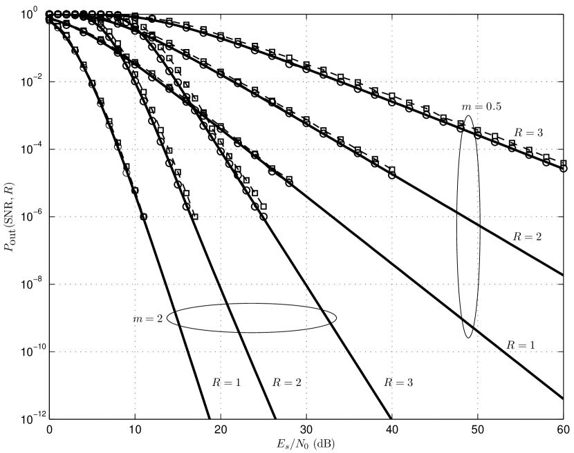
Figure 1: Outage probability of Nakagami-$m$ block-fading channels with $B=4,M=4$, $m=0.5$ and $m=2$. The thick solid lines correspond to the lower bound (28), thin dashed lines with circles denote the simulation of (19) and thin dashed lines with squares denote the simulation of (9) with $16$-QAM modulation.

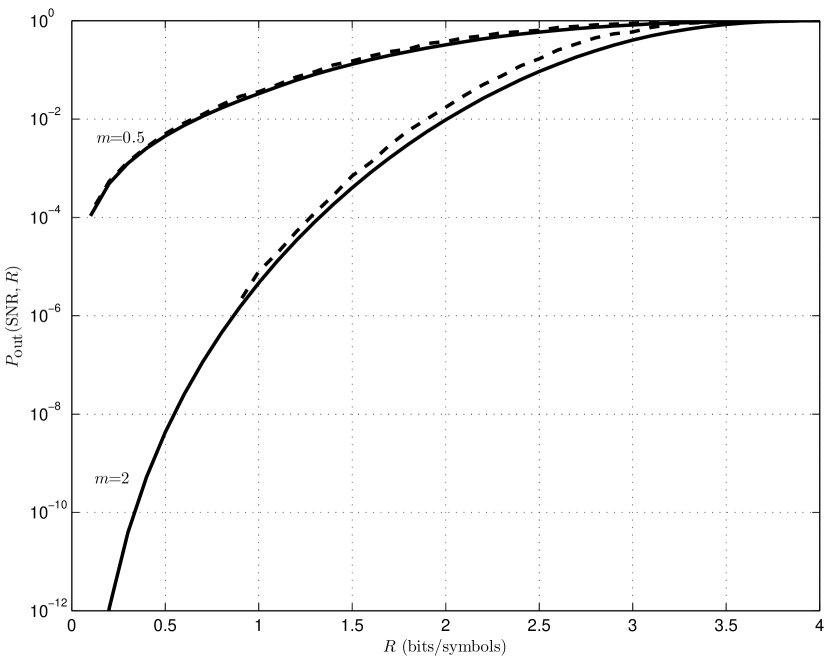
Figure 2: Outage probability for the of Nakagami-$m$ block-fading channels with $B=4,M=4,{\rm SNR}=10{\rm dB}$, $m=0.5$ and $m=2$. The solid lines correspond to the lower bound (28). The dashed lines denote the simulation of (9) with 16-QAM modulation.

Numerical results for Nakagami-$m$ block-fading channels with $B=4$, $M=4$, $m=0.5$ and $m=2$ are given in Figure 1. The transmission rates considered are $R=1,2,3$ bits per channel use, which correspond to Singleton bounds $d_{B}(R)=4,3,2$, respectively. The figure shows the simulation and analytical curves of the lower bound to the outage probability of the channel based on (19) and (28), respectively, together with the 16-QAM outage simulation curve based on (9). We observe that the analytical curves coincide with the corresponding lower bound simulation curves. The analytical curves give a tight lower bound to the 16-QAM outage curve. Note that the bound is very tight for the important case of $R=1$, which, from the Singleton bound expression in (2), is the largest rate that can be achieved with full diversity. Figure 2 provides a plot of the outage probability of the same channels as a function of the code rate $R$ at ${\rm SNR}=10$dB, illustrating the validity of the bound over a wide range of transmission rates. Further simulations show that these observations are valid for a wide range of channel parameters. We also observe from Figure 1 that the slope of each curve is $md_{B}(R)$, representing the SNR exponent of the outage probability. In the following section, we rigorously prove that the optimal SNR-exponent over the channel is

$$d^{\star}(R)=md_{B}(R).$$ (29)

In proving this result, we characterize not only the SNR-exponent but also the asymptotic coding gain.

V Asymptotic Behavior

Using (28) and the analysis techniques from [8], we obtain the following result for the asymptotic diversity of Nakagami-$m$ block-fading channels, for all $m>0$.

Proposition 2

Assume transmission over the block-fading channel as defined in (4) with input signal constellation size $2^{M}$. Assume further that the fading power gain $\gamma_{b}$ is a random variable whose distribution is given by (6). In this case, the lower bound on $P_{\rm out}({\rm SNR},R)$ given in (28) can asymptotically be expressed as

$$P^{\ell}_{\rm out}({\rm SNR},R)\doteq\mathcal{K}_{\ell}{\rm SNR}^{-md_{B}(R)},$$ (30)

where $d_{B}(R)$ is the Singleton bound given in (2). Furthermore, $\mathcal{K}_{\ell}$ is a constant independent of ${\rm SNR}$ given by

$$\mathcal{K}_{\ell}=F_{\overline{Y}_{B-d_{B}(R)}}\Big{(}BR-(B-d_{B}(R))M\Big{)}\binom{B}{B-d_{B}(R)}\frac{(m(2^{M}-1))^{md_{B}(R)}}{(m\Gamma(m))^{d_{B}(R)}},$$ (31)

where

$$F_{\overline{Y}_{t}}(\xi)=\lim_{{\rm SNR}\to\infty}F_{Y_{t}}(\xi)$$ (32)

Proof:

See Appendix B. ∎

This proposition not only shows that the SNR exponent of the outage probability is upper bounded by $md_{B}(R)$ but also gives the asymptotic constant $\mathcal{K}_{\ell}$ of $P^{\ell}_{\rm out}({\rm SNR},R)$. This is indeed useful for code design since it gives an upper bound for the coding gain achieved by any coding scheme. At the same time, together with the expression of $P_{\rm out}^{\ell}({\rm SNR},R)$ given in (28), it gives a more specific characterization of the outage probability, indicating the word error probability (or SNR) region where asymptotic analysis is valid.

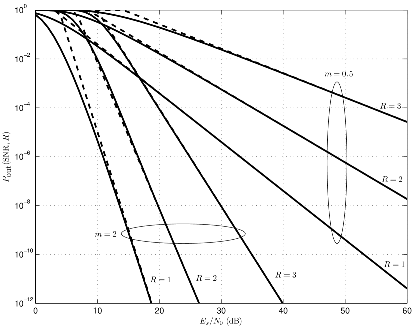
Figure 3: Outage probability of Nakagami-$m$ block-fading channels with $B=4,M=4$, $m=0.5$ and $m=2$. The solid lines correspond to the lower bound (28) and the dashed lines to its asymptotic expression given in (30) using $\mathcal{K}_{\ell}$ in (31).

The lower bound to the outage probability and the asymptotic term given in (30) are illustrated in Figure 3. The same set of parameters as in Figure 1 has been chosen, namely $B=4,M=4,m=2$ and $R=1,2,3$.

So far, we have shown that $d^{\star}(R)\leq md_{B}(R)$. To prove the optimality of the SNR-exponent $md_{B}(R)$, we need to prove the achievability result given in the next proposition.

Proposition 3

Assume transmission with random codes of rate $R$ and block length $L({\rm SNR})$ satisfying

$$\lim_{{\rm SNR}\to\infty}\frac{L({\rm SNR})}{\log({\rm SNR})}=\lambda$$ (33)

over a block-fading channel as defined in (4) with input signal constellation size $2^{M}$. Further assume that the fading power gain $\gamma_{b}$ is a random variable whose distribution is given by (6). In this case, the SNR-exponent is lower bounded by

$$d^{(r)}(R)\geq\left\{\begin{array}[]{ll}\lambda BM\log(2)(1-\frac{R}{M}),&\lambda<\frac{m}{M\log(2)}\\ m(d_{B}(R)-1)+\min\left\{m,\lambda M\log(2)\left(B\left(1-\frac{R}{M}\right)-d_{B}(R)+1\right)\right\},&\lambda\geq\frac{m}{M\log(2)}.\end{array}\right.$$ (34)

Proof:

See Appendix C. ∎

The preceding propositions lead to the following theorem.

Theorem 1

Assume transmission over a block-fading channel as defined in (4) with input constellation size $2^{M}$. Further assume that the fading power gain $\gamma_{b}$ is a random variable whose distribution is given by (6). In this case, the optimal SNR-exponent is given by

$$d^{\star}(R)=md_{B}(R)$$ (35)

for all $R,M$ where $B\left(1-\frac{R}{M}\right)$ is not an integer.

Proof:

See Appendix D. ∎

As remarked in Appendix D, Theorem 1 can be proved using the methods proposed in [8]. However, with the proof proposed here, Propositions 2 and 3 provide additional information. In particular, Proposition 2 provides an upper bound on the coding gain $\mathcal{K}_{\ell}$, and Proposition 3 provides an extension for the SNR-exponent of random codes with finite block length in [8] to a more general fading distribution.

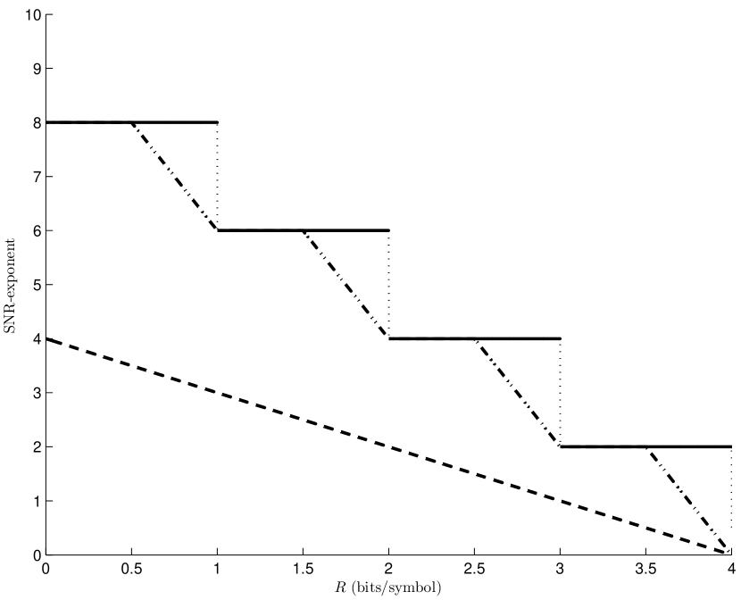
Figure 4: Optimal and random coding SNR-exponent for Nakagami-$m$ block-fading channels with $m=2,B=4,M=4$. The solid line corresponds to $md_{B}(R)$, dashed-dotted line and dashed line denote the random coding exponent with $\lambda M\log(2)=2m$ and $\lambda M\log(2)=\frac{m}{2}$ respectively.

The diversity of random codes for block-fading channels with $B=4$, $M=4$ and $m=2$ is illustrated in Figure 4. Random codes with block length satisfying $\lambda=\frac{2m}{M\log(2)}$ and $\lambda=\frac{m}{2M\log(2)}$ are considered, where $\lambda$ is defined in (33). We observe that the SNR-exponent is always upper bounded by $md_{B}(R)$. Except for points of discontinuity of $d_{B}(R)$, the upper bound can be achieved by increasing $\lambda$ since $d^{(r)}(R)$ and $md_{B}(R)$ will coincide over larger ranges of $R$.

VI Conclusion

In this correspondence, we have proposed a tight lower bound to the outage probability of discrete-input block-fading channels with Nakagami-$m$ fading statistics. The lower bound can be computed efficiently and is therefore useful for system design and analysis. We show that the optimal rate-diversity trade-off for Nakagami-$m$ block-fading channels is given by $m$ times the Singleton bound. We also obtain an upper bound for the achievable coding gain, which is useful for code design.

Appendix A Distribution and Properties of $A_{b}$

Proposition 1

Assume $\gamma_{b}$ is a random variable whose distribution is given by (6). Denote $A_{b}$ the random variable $\log_{2}(1+\gamma_{b}{\rm SNR})$ conditioned on the event $\mathcal{E}$ described in (22). The distribution of $A_{b}$, is given by

$$f_{A_{b}}(\xi)=\left\{\begin{array}[]{ll}\frac{f_{\gamma_{b}}\left(\frac{2^{\xi}-1}{{\rm SNR}}\right)}{F_{\gamma_{b}}\left(\frac{2^{M}-1}{{\rm SNR}}\right)}\frac{2^{\xi}\log(2)}{{\rm SNR}},&0\leq\xi\leq M\\ 0,&\rm{otherwise}.\end{array}\right.$$ (36)

Proof:

The cdf of $A_{b}$ is given by

$$F_{A_{b}}(\xi) =\Pr(\log_{2}(1+\gamma_{b}{\rm SNR})<\xi|\mathcal{E})$$ (37)

$$=\Pr\left(\log_{2}(1+\gamma_{b}{\rm SNR})<\xi\left|\gamma_{b}\leq\frac{2^{M}-1}{{\rm SNR}}\right.\right).$$ (38)

Applying Bayes’ rule, we obtain

$$F_{A_{b}}(\xi)=\frac{\Pr\left(\gamma_{b}<\frac{2^{\xi}-1}{{\rm SNR}},\gamma_{b}\leq\frac{2^{M}-1}{{\rm SNR}}\right)}{\Pr\left(\gamma_{b}\leq\frac{2^{M}-1}{{\rm SNR}}\right)}.$$ (39)

If $\xi\leq M$ then $2^{\xi}-1\leq 2^{M}-1$ and therefore,

$$\Pr\left(\gamma_{b}<\frac{2^{\xi}-1}{{\rm SNR}},\gamma_{b}\leq\frac{2^{M}-1}{{\rm SNR}}\right) = \Pr\left(\gamma_{b}<\frac{2^{\xi}-1}{{\rm SNR}}\right)$$ (40)

$$= F_{\gamma_{b}}\left(\frac{2^{\xi}-1}{{\rm SNR}}\right).$$ (41)

Otherwise, if $\xi>M$,

$$\Pr\left(\gamma_{b}<\frac{2^{\xi}-1}{{\rm SNR}},\gamma_{b}\leq\frac{2^{M}-1}{{\rm SNR}}\right) = \Pr\left(\gamma_{b}\leq\frac{2^{M}-1}{{\rm SNR}}\right)$$ (42)

$$= F_{\gamma_{b}}\left(\frac{2^{M}-1}{{\rm SNR}}\right).$$ (43)

By inserting (41) and (43) into (39), we finally have that

$$F_{A_{b}}(\xi)=\left\{\begin{array}[]{ll}\frac{F_{\gamma_{b}}\left(\frac{2^{\xi}-1}{{\rm SNR}}\right)}{F_{\gamma_{b}}\left(\frac{2^{M}-1}{{\rm SNR}}\right)},&\xi\leq M\\ 1,&\mbox{otherwise}.\end{array}\right.$$ (44)

Now differentiate $F_{A_{b}}(\xi)$ in (44) with respect to $\xi$, noting that $\frac{d}{d\xi}F_{A_{b}}(\xi)=f_{A_{b}}(\xi)$ and $\frac{d}{d\xi}F_{\gamma_{b}}(\xi)=f_{\gamma_{b}}(\xi)$, we obtain (23). ∎

Proposition 4

Assume $\gamma_{b}$ is a random variable whose distribution is given by (6). Assume $A_{b}$ is a random variable as defined in Proposition 1. Asymptotically, the distribution of $A_{b}$ is independent of ${\rm SNR}$ and is given by

$$f_{A_{b}}(\xi)\doteq f_{\overline{A}_{b}}(\xi)\triangleq\left\{\begin{array}[]{ll}\frac{m(2^{\xi}-1)^{m-1}2^{\xi}\log(2)}{(2^{M}-1)^{m}},&\xi\leq M,\\ 0,&\rm{otherwise}.\end{array}\right.$$ (45)

Proof:

From (6) and Taylor series expansion, we have

$$f_{\gamma_{b}}\left(\frac{2^{\xi}-1}{{\rm SNR}}\right) = \frac{m^{m}\left(\frac{2^{\xi}-1}{{\rm SNR}}\right)^{m-1}}{\Gamma(m)}e^{-m\frac{2^{\xi}-1}{{\rm SNR}}}$$ (46)

$$\doteq \frac{m^{m}(2^{\xi}-1)^{m-1}}{\Gamma(m)}{\rm SNR}^{-(m-1)}.$$

Similarly, from (7), we have

$$F_{\gamma_{b}}\left(\frac{2^{M}-1}{{\rm SNR}}\right) = 1-\frac{\Gamma\left(m,m\frac{2^{M}-1}{{\rm SNR}}\right)}{\Gamma(m)}$$ (47)

$$\doteq 1-\frac{\Gamma(m)-\frac{1}{m}\left(m\frac{2^{M}-1}{{\rm SNR}}\right)^{m}}{\Gamma(m)}$$

$$\doteq \frac{m^{m}(2^{M}-1)^{m}}{m\Gamma(m)}{\rm SNR}^{-m}.$$

Inserting (46) and (47) into (36), we obtain (45). ∎

Appendix B Proof of Proposition 2

Define $\overline{A}_{k}$ as a random variable described by the distribution function $f_{\overline{A}_{b}}(\xi)$ given in (45). Further define $F_{\overline{Y}_{t}}(\xi)$ as the cdf of $\overline{Y}_{t}\triangleq\sum_{k=1}^{B-t}\overline{A}_{k}$. According to Proposition 4, $f_{A_{b}}(\xi)\doteq f_{\overline{A}_{b}}(\xi)$, and therefore, $F_{Y_{t}}(\xi)\doteq F_{\overline{Y}_{t}}(\xi)$. In addition, Taylor expansion of (18) gives

$$p \doteq \frac{\Gamma(m)-\frac{1}{m}(m\frac{2^{M}-1}{{\rm SNR}})^{m}}{\Gamma(m)}\doteq 1,$$ (48)

$$1-p \doteq \frac{m^{m}(2^{M}-1)^{m}}{m\Gamma(m)}{\rm SNR}^{-m}.$$ (49)

Since the asymptotic expressions for $p,1-p$ and $F_{Y_{t}}(\xi)$ are finite and non-zero, the asymptotic behavior of $P^{\ell}_{\rm out}({\rm SNR},R)$ in (28) is found by replacing $F_{Y_{t}}(\xi)$ with $F_{\overline{Y}_{t}}(\xi)$, and replacing $p,1-p$ with their corresponding asymptotic value in (48) and (49). It follows that

$$P^{\ell}_{\rm out}({\rm SNR},R)\doteq\sum_{t=0}^{\left\lceil\frac{BR}{M}\right\rceil-1}F_{\overline{Y}_{t}}(BR-tM)\binom{B}{t}\left(\frac{m^{m}(2^{M}-1)^{m}}{m\Gamma(m)}\right)^{B-t}{\rm SNR}^{-m(B-t)}.$$ (50)

Since $f_{\overline{A}_{b}}(\xi)$ is independent of ${\rm SNR}$, $F_{\overline{Y}_{t}}(\xi)$ is also independent of ${\rm SNR}$. Therefore, the term with minimum $m(B-t)$ dominates the expression in (50). The dominating term corresponds to

$$t=\left\lceil\frac{BR}{M}\right\rceil-1,$$ (51)

and thus

$$B-t=1+\left\lfloor B\left(1-\frac{R}{M}\right)\right\rfloor=d_{B}(R),$$ (52)

which is precisely the Singleton bound. Therefore, we write the asymptotic behavior for (28) as

$$P^{\ell}_{\rm out}({\rm SNR},R)\doteq\mathcal{K}_{\ell}\,{\rm SNR}^{-md_{B}(R)},$$ (53)

where

$$\mathcal{K}_{\ell}=F_{\overline{Y}_{B-d_{B}(R)}}\Big{(}BR-(B-d_{B}(R))M\Big{)}\binom{B}{B-d_{B}(R)}\frac{(m(2^{M}-1))^{md_{B}(R)}}{(m\Gamma(m))^{d_{B}(R)}}$$ (54)

is independent of ${\rm SNR}$.

Appendix C Proof of Proposition 3

The proof follows the same lines as in [8] with the generalization of Rayleigh fading statistic to Nakagami-$m$ fading statistic.

Defining the normalized fading gains as in [15]

$$\alpha_{b}=-\frac{\log\gamma_{b}}{\log({\rm SNR})},$$ (55)

we have the following result.

Proposition 5

Assume $\gamma_{b}$ is a random variable with distribution in (6). Assume further that $\alpha_{b}$ is a random variable as defined in (55). In this case, the joint distribution of $\mbox{\boldmath{$\alpha$}}=(\alpha_{1},\ldots,\alpha_{B})$ has the following asymptotic behavior

$$f_{\mbox{\boldmath{$\alpha$}}}(\mbox{\boldmath{$\alpha$}})\doteq\left\{\begin{array}[]{ll}{\rm SNR}^{-m\sum_{b=1}^{B}\alpha_{b}},&\mbox{\boldmath{$\alpha$}}\in\mathbb{R}^{B}_{+}\\ 0,&\rm{otherwise}.\end{array}\right.$$ (56)

Proof:

From (55), $\gamma_{b}={\rm SNR}^{-\alpha_{b}}$. Therefore, the pdf of $\alpha_{b}$ is

$$f_{\alpha_{b}}(\alpha_{b}) = f_{\gamma_{b}}\left({\rm SNR}^{-\alpha_{b}}\right)\left|\frac{d\gamma_{b}}{d\alpha_{b}}\right|$$ (57)

$$= \frac{m^{m}{\rm SNR}^{-(m-1)\alpha_{b}}\exp(-m{\rm SNR}^{-\alpha_{b}})}{\Gamma(m)}{\rm SNR}^{-\alpha_{b}}\log{\rm SNR}$$

$$= \frac{m^{m}}{\Gamma(m)}{\rm SNR}^{-m\alpha_{b}}\exp(-m{\rm SNR}^{-\alpha_{b}})\log({\rm SNR}).$$

The joint distribution of the vector $\alpha$ is then

$$f_{\mbox{\boldmath{$\alpha$}}}(\mbox{\boldmath{$\alpha$}})=\left(\frac{m^{m}\log({\rm SNR})}{\Gamma(m)}\right)^{B}{\rm SNR}^{-m\sum_{b=1}^{B}\alpha_{b}}\exp\left(-m\sum_{b=1}^{B}{\rm SNR}^{-\alpha_{b}}\right).$$ (58)

It can easily be seen that

$$\lim_{{\rm SNR}\rightarrow\infty}\frac{\log(f_{\mbox{\boldmath{$\alpha$}}}(\mbox{\boldmath{$\alpha$}}))}{\log({\rm SNR})}=\left\{\begin{array}[]{ll}-m\sum_{b=1}^{B}\alpha_{b},&\mbox{\boldmath{$\alpha$}}\in\mathbb{R}^{B}_{+}\\ 0,&\rm{otherwise}.\end{array}\right.$$ (59)

Therefore, $f_{\mbox{\boldmath{$\alpha$}}}(\mbox{\boldmath{$\alpha$}})$ follows the asymptotic behavior in (56). ∎

Consider random codes of rate $R$ and block length $L=L({\rm SNR})$ over a signal set of size $2^{M}$ such that

$$\lambda=\lim_{{\rm SNR}\rightarrow\infty}\frac{L({\rm SNR})}{\log({\rm SNR})}.$$ (60)

Assume the codewords of the code are given by $\mathbf{X}(i),i=0,\ldots,2^{BLR}-1$. Following the analysis in [8], the average pairwise error probability between $\mathbf{X}(0)$ and $\mathbf{X}(1)$ for a given channel realization $\mathbf{h}$ is given by

$$\overline{P(\mathbf{X}(0)\to\mathbf{X}(1)|\mathbf{h})}\leq\prod_{b=1}^{B}\beta_{b}^{L},$$ (61)

where $\beta_{b}$ is the Bhattacharrya coefficient

$$\beta_{b}=2^{-2M}\sum_{x\in\mathcal{X}}\sum_{x^{\prime}\in\mathcal{X}}\exp\left(-\frac{{\rm SNR}}{4}\gamma_{b}|x-x^{\prime}|^{2}\right).$$ (62)

The union bound of the word error probability for a given fading coefficient is obtained by summing over the pairwise error probability of $2^{BLR}-1$ codewords $\mathbf{X}(i),i=1,\ldots,2^{BLR}-1$. Noting that $\gamma_{b}={\rm SNR}^{1-\alpha_{b}}$, we obtain

$$\overline{P_{e}({\rm SNR}|\mathbf{h})}$$

$$\leq\exp\left(-BLM\log(2)\left[1-\frac{R}{M}-\frac{1}{BM}\sum_{b=1}^{B}\log_{2}\left(1+2^{-M}\sum_{x\neq x^{\prime}}e^{-\frac{1}{4}|x-x^{\prime}|^{2}{\rm SNR}^{1-\alpha_{b}}}\right)\right]\right)$$ (63)

$$=\exp(-BLM\log(2)G({\rm SNR},\mbox{\boldmath{$\alpha$}})).$$ (64)

Using (64) and the fact that $\overline{P_{e}({\rm SNR}|\mathbf{h})}\leq 1$, the average error probability is given by

$$\overline{P_{e}({\rm SNR})}\leq\int_{\mbox{\boldmath{$\alpha$}}}\min\{1,\exp(-BLM\log(2)G({\rm SNR},\mbox{\boldmath{$\alpha$}}))\}f_{\mbox{\boldmath{$\alpha$}}}(\mbox{\boldmath{$\alpha$}})d\mbox{\boldmath{$\alpha$}}.$$ (65)

Now, from Proposition 5, we have

$$\overline{P_{e}({\rm SNR})}\dot{\leq}\int_{\mbox{\boldmath{$\alpha$}}\in\mathbb{R}^{N}_{+}}{\rm SNR}^{-m\sum_{b=1}^{B}\alpha_{b}}\min\{1,\exp(-BLM\log(2)G({\rm SNR},\mbox{\boldmath{$\alpha$}}))\}d\mbox{\boldmath{$\alpha$}}.$$ (66)

Noting that

$$\lim_{{\rm SNR}\to\infty}\log_{2}\left(1+2^{-M}\sum_{x\neq x^{\prime}}e^{-\frac{1}{4}|x-x^{\prime}|^{2}{\rm SNR}^{1-\alpha_{b}}}\right)=\left\{\begin{array}[]{ll}0,&\alpha_{b}<1\\ M,&\alpha_{b}>1,\end{array}\right.$$ (67)

we can replace $G({\rm SNR},\mbox{\boldmath{$\alpha$}})$ in (66) by

$$\tilde{G}_{\epsilon}(\mbox{\boldmath{$\alpha$}})=1-\frac{R}{M}-\frac{1}{B}\sum_{b=1}^{B}\leavevmode\hbox{\small 1\normalsize\kern-3.30002pt1}\{\alpha_{n}\geq 1-\epsilon\}$$ (68)

for any $\epsilon>0$. Therefore, by defining

$$\mathcal{B}_{\epsilon}=\left\{\mbox{\boldmath{$\alpha$}}:\tilde{G}_{\epsilon}(\mbox{\boldmath{$\alpha$}})\leq 0\right\}$$ (69)

and $\mathcal{B}_{\epsilon}^{c}$ as the complement of $\mathcal{B}_{\epsilon}$, we can write (66) as

$$P_{e}({\rm SNR})\dot{\leq} \int_{\mathcal{B}_{\epsilon}\cap\mathbb{R}_{+}^{B}}{\rm SNR}^{-m\sum_{b=1}^{B}\alpha_{b}}d\mbox{\boldmath{$\alpha$}}$$ (70)

$$+ \int_{\mathcal{B}_{\epsilon}^{c}\cap\mathbb{R}_{+}^{B}}\exp\left(-\log({\rm SNR})\left(m\sum_{b=1}^{B}\alpha_{b}+B\lambda M\log(2)\tilde{G}_{\epsilon}(\mbox{\boldmath{$\alpha$}})\right)\right)d\mbox{\boldmath{$\alpha$}}.$$

By applying the Varadhan’s lemma, the SNR-exponents of the first and second term in (70) are given by

$$\inf_{\mbox{\boldmath{$\alpha$}}\in\mathcal{B}_{\epsilon}\cap\mathbb{R}_{+}^{B}}\left\{m\sum_{b=1}^{B}\alpha_{b}\right\}\;\;\;\;{\rm and}\;\;\;\inf_{\mbox{\boldmath{$\alpha$}}\in\mathcal{B}_{\epsilon}^{c}\cap\mathbb{R}_{+}^{B}}\left\{m\sum_{b=1}^{B}\alpha_{b}+B\lambda M\log(2)\tilde{G}_{\epsilon}(\mbox{\boldmath{$\alpha$}})\right\},$$

respectively. Therefore, the SNR-exponent of the word error probability is given by

$$d^{(r)}(R)\geq\sup_{\epsilon>0}\min\left\{\inf_{\mbox{\boldmath{$\alpha$}}\in\mathcal{B}_{\epsilon}\cap\mathbb{R}_{+}^{B}}\left\{m\sum_{b=1}^{B}\alpha_{b}\right\},\inf_{\mbox{\boldmath{$\alpha$}}\in\mathcal{B}_{\epsilon}^{c}\cap\mathbb{R}_{+}^{B}}\left\{m\sum_{b=1}^{B}\alpha_{b}+B\lambda M\log(2)\tilde{G}_{\epsilon}(\mbox{\boldmath{$\alpha$}})\right\}\right\}.$$ (71)

For the first infimum in (71), it can be shown that

$$\inf_{\mbox{\boldmath{$\alpha$}}\in\mathcal{B}_{\epsilon}\cap\mathbb{R}_{+}^{B}}\left\{m\sum_{b=1}^{B}\alpha_{b}\right\}=m(1-\epsilon)\left\lceil B\left(1-\frac{R}{M}\right)\right\rceil.$$ (72)

The infimum is attained when $\left\lceil B\left(1-\frac{R}{M}\right)\right\rceil$ entries of $\alpha$ are $1-\epsilon$, and the other entries are zero.
The second infimum in (71) can be rewritten as

$$B\lambda M\log(2)\left(1-\frac{R}{M}\right)+\inf_{\mbox{\boldmath{$\alpha$}}\in\mathcal{B}_{\epsilon}^{c}\cap\mathbb{R}_{+}^{B}}\left\{\sum_{b=1}^{B}m\alpha_{b}-\lambda M\log(2)\leavevmode\hbox{\small 1\normalsize\kern-3.30002pt1}\{\alpha_{b}\geq 1-\epsilon\}\right\}.$$ (73)

We consider two cases. If $0\leq\lambda M\log(2)<m$, the infimum in (73) is zero and achieved when $\mbox{\boldmath{$\alpha$}}=\mathbf{0}$. Therefore, the second infimum in (71) is given by

$$B\lambda M\log(2)\left(1-\frac{R}{M}\right).$$ (74)

If $\lambda M\log(2)\geq m$, the infimum in (73) is given by

$$(m(1-\epsilon)-\lambda M\log(2))\left\lfloor B\left(1-\frac{R}{M}\right)\right\rfloor.$$ (75)

The infimum is attained when $\left\lfloor B\left(1-\frac{R}{M}\right)\right\rfloor$ entries of $\alpha$ are $1-\epsilon$, and the other entries are zero. Hence, the second infimum in (71) is given by

$$B\lambda M\log(2)\left(1-\frac{R}{M}\right)+(m(1-\epsilon)-\lambda M\log(2))\left\lfloor B\left(1-\frac{R}{M}\right)\right\rfloor.$$ (76)

By collecting the results, and noting that the supremum in (71) is attained when $\epsilon\downarrow 0$, we obtain the lower bound for the SNR-exponent as in (34).

Appendix D Proof of Theorem 1

Clearly $P_{\rm out}({\rm SNR},R)\geq P^{\ell}_{\rm out}({\rm SNR},R)$, and therefore,

$$d^{\star}_{B}(R)\leq md_{B}(R)$$ (77)

follows from Proposition 2. In addition, by letting $L({\rm SNR})\rightarrow\infty$, it follows from Proposition 3 that the SNR-exponent $md_{B}(R)$ is achievable using random codes for all $R,M$ such that $B\left(1-\frac{R}{M}\right)$ is not an integer. ∎

The theorem can also be proved using the SNR-normalized fading coefficients $\alpha_{b}\triangleq-\frac{\log(\gamma_{b})}{\log({\rm SNR})}$ introduced in [15]. The proof given in [8] for the Rayleigh fading case ($m=1$) shows that the asymptotic behavior of the joint pdf of these coefficients is $f_{\mbox{\boldmath{$\alpha$}}}(\mbox{\boldmath{$\alpha$}})\doteq{\rm SNR}^{-\sum_{b=1}^{B}\alpha_{b}}$ and thus

$$d^{\star}(R)\leq\inf_{\mathcal{B}_{1}}\left\{\sum_{b=1}^{B}\alpha_{b}\right\}=d_{B}(R)$$ (78)

and

$$d^{\star}(R)\geq\inf_{\mathcal{B}_{2}}\left\{\sum_{b=1}^{B}\alpha_{b}\right\}=d_{B}(R),$$ (79)

whenever $B\left(1-\frac{R}{M}\right)$ is not an integer, for some suitably defined sets $\mathcal{B}_{1},\mathcal{B}_{2}$ (see [8] for details). In Proposition 5, it is shown that for Nakagami-$m$ distributions the asymptotic behavior of the joint pdf of these coefficients behaves as $f_{\mbox{\boldmath{$\alpha$}}}(\mbox{\boldmath{$\alpha$}})\doteq{\rm SNR}^{-m\sum_{b=1}^{B}\alpha_{b}}$. In this case, the constant $m$ factors out from the infimums in (78) and (79) and automatically leads to the desired result. While this proof is shorter, Proposition 3 provides the extension of the finite block length results of [8], which illustrates the impact of $m$ in the random SNR-exponent $d^{(r)}(R)$.

References

• [1] L. H. Ozarow, S. Shamai, and A. D. Wyner, “Information theoretic considerations for cellular mobile radio,” IEEE Trans. Veh. Tech., vol. 43, no. 2, pp. 359–378, May 1994.
• [2] E. Biglieri, J. Proakis, and S. Shamai, “Fading channels: Informatic-theoretic and communications aspects,” IEEE Trans. Inf. Theory, vol. 44, no. 6, pp. 2619–2692, Oct. 1998.
• [3] S. Verdú and T. S. Han, “A general formula for shannon capacity,” IEEE Trans. Inf. Theory, vol. 40, no. 4, pp. 1147–1157, Jul. 1994.
• [4] G. Caire, G. Taricco, and E. Biglieri, “Optimal power control over fading channels,” IEEE Trans. Inf. Theory, vol. 45, no. 5, pp. 1468–1489, Jul. 2001.
• [5] E. Malkamäki, “Performance of error control over block fading channels with ARQ applications,” Ph.D. dissertation, Helsinki Univ. Technology, Helsinki, Finland, 1998.
• [6] E. Malkamäki and H. Leib, “Coded diversity on block-fading channels,” IEEE Trans. Inf. Theory, vol. 45, no. 2, pp. 771–781, Mar. 1999.
• [7] R. Knopp and P. A. Humblet, “On coding for block fading channels,” IEEE Trans. Inf. Theory, vol. 46, no. 1, pp. 189–205, Jan. 2000.
• [8] A. Guillén i Fàbregas and G. Caire, “Coded modulation in the block-fading channel: Coding theorems and code construction,” IEEE Trans. Inf. Theory, vol. 52, no. 1, pp. 91–114, Jan. 2006.
• [9] E. Baccarelli, “Asymptotic tight bounds on the capacity and outage probability for QAM transmission over Rayleigh-faded data channels with CSI,” IEEE Trans. Commun., vol. 47, no. 9, pp. 1273–1277, Sep. 1999.
• [10] E. Baccarelli and A. Fasano, “Some simple bounds on the symmetric capacity and outage probability for QAM wireless channels with Rice and Nakagami fadings,” IEEE Trans. Veh. Tech., vol. 18, no. 3, pp. 361–368, Mar. 2000.
• [11] M. Nakagami, “The $m$-distribution - a general formula of intensity distribution of rapid fading,” in Statistical Methods in Radio Wave Propagation, W. G. Hoffman, Ed.   Oxford: Pergamon Press, 1960, pp. 3–36.
• [12] M. K. Simon and M. S. Alouini, Digital Communications over Fading Channels, 2nd ed.   John Wiley and Sons, 2004.
• [13] M. Abramowitz and I. A. Stegun, Handbook of Mathematical Functions with Formulas, Graphs, and Mathematical Tables.   New York: Dover, 1964.
• [14] J. G. Proakis and D. G. Manolakis, Digital signal processing : principles, algorithms, and applications, 2nd ed.   New York : Macmillan, 1992.
• [15] L. Zheng and D. N. Tse, “Diversity and multiplexing: A fundamental tradeoff in multiple-antenna channels,” IEEE Trans. Inf. Theory, vol. 49, no. 5, pp. 1073–1096, May. 2003.
• [16] T. M. Cover and J. A. Thomas, Elements of Information Theory, 2nd ed.   John Wiley and Sons, 2006.