The Analysis of Penumbral Fine Structure Using an Advanced Inversion Technique

Abstract

We present a method to study the penumbral fine structure using data obtained by the spectropolarimeter onboard HINODE. For the first time, the penumbral filaments can be considered as resolved in spectropolarimetric measurements. This enables us to use inversion codes with only one-component model atmospheres, and thus assign the obtained stratifications of plasma parameters directly to the penumbral fine structure. This approach is applied to the limb-side part of the penumbra in active region NOAA 10923. The preliminary results show a clear dependence of the plasma parameters on continuum intensity in the inner penumbra, i.e. weaker and horizontal magnetic field along with increased line-of-sight velocity are found in the low layers of the bright filaments. The results in the mid penumbra are ambiguous and future analyses are necessary to unveil the magnetic field structure and other plasma parameters there.

1 Introduction

Although the fine structure of penumbra has been studied for a long time, there are only a few confirmed facts regarding the plasma properties and origin of penumbral filaments. However, the global properties of the magnetic and velocity structure of the penumbra are well known, i.e. the magnetic field becomes weaker and more horizontal with increasing distance from the sunspot umbra and the velocity field is composed mostly of horizontally oriented Evershed flow, which points outward at photospheric layers (see the review by Solanki, 2003, and references therein).

Differences in the plasma parameters of bright and dark filaments were reported for the first time by Beckers & Schröter (1969) who found stronger and more vertical fields in dark filaments. With increasing spatial resolution came other observations that confirmed the rapid changes of inclination and magnetic filed strength on arcsec and sub-arcsec scales (see Solanki, 2003, and references therein).

However, the properties of the filamentary structure of the penumbra have been derived indirectly from spectropolarimetric measurements (by means of two-component model atmospheres) due to the relatively poor spatial resolution attained by ground-based instruments (see e.g. Bellot Rubio et al., 2004, 2006; Borrero et al., 2004, 2006). These analyses found weaker and more horizontal magnetic fields associated with increased velocities, but these properties cannot be ascribed to specific intensity structures due to the lack of spatial resolution.

Spectroscopic observations at 0.2^′′ resolution have revealed some properties of bright penumbral filaments (Bellot Rubio et al., 2005) which are consistent with the indirect analyses described above. Similar results were obtained also by Langhans et al. (2005) who analysed one-wavelength magnetograms at the same resolution. A direct determination of the vector magnetic field of penumbral filaments can be done for the first time using the spectropolarimetric data obtained by HINODE Solar Optical Telescope (SOT).

In this paper, we describe the observations, data reduction, and the inversion method used for a detailed analysis of the penumbral structure. Hopefully, our results will help to distinguish between competitive models of the penumbra (see BellotRubio, 2007, for a review).

2 Observations

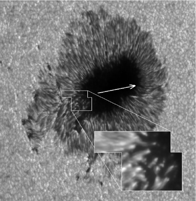
Figure 1: The map of continuum intensity reconstructed from the red wing of the Fe I 630.25 nm line. The area under analysis is highlighted and the arrow points to disc centre.

We analyse data obtained using the spectropolarimeter (SP; Tarbell, 2007) which is part of the Solar Optical Telescope (SOT; Tsuneta, 2007) onboard the HINODE satellite (Kosugi, 2007).

The instrument observes the two iron lines Fe I 630.15 nm (Landé factor $g=1.67$) and Fe I 630.25 nm ($g=2.5$). The diffraction limit of SOT is 0.3^′′ at 630 nm. The width of the spectrograph slit is equivalent to 0.16^′′ matching the pixel size of the CCD camera. The scanning steps of the spectrograph slit is equivalent to 0.148^′′. The wavelength sampling of 2.15 pm is finer than the spectral resolution of 2.5 pm. The exposure time for one slit position is 4.8 s, during which all Stokes profiles are acquired with a noise level of $10^{-3}I_{c}$. The spatial resolution is slightly worse than the diffraction limit of the telescope due to the aliasing induced by the CCD pixel size, but it nevertheless reaches 0.32^′′.

The dark-field substraction, the flat-field division, the instrumental polarisation correction, and other data reductions are made using the calibration software developed by B. Lites. To prepare the data for the inversion process, a calibration of wavelengths and a normalisation of the Stokes profiles to the continuum intensity of the Harvard Smithsonian reference atmosphere (HSRA) must be done. We perform this calibration for each slit position separately using the pixels along the slit with weak polarisation signal. The minimum of the Fe I 630.15 nm Stokes $I$ profile averaged over these pixels is used for the definition of zero velocity and the continuum intensity of this profile is normalised to HSRA as unity (times the appropriate limb-darkening factor). Following this approach, the photospheric 5 minute oscillations are suppressed to the extent that we do not see any oscillations in the resulting maps of line-of-sight (LOS) velocity.

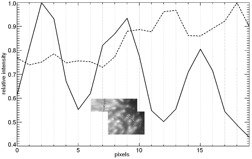
Figure 2: Two cuts through the filamentary structure of the penumbra are marked in the intensity map in the lower part of the figure. The continuum intensity along these cuts are shown in the plot where the solid and dashed lines correspond to the cuts through the inner and mid penumbra respectively.

On November 10, 2006, the spot in AR 10923 located at heliocentric position 49^∘ E and 6^∘ S (heliocentric angle $\mu=0.65$) was observed. The observed region is shown in figure 1, where the highlighted area in size of $14\times 10$ arcsec is analysed. The arrow points to the disc centre.

In figure 2 we demonstrate that the penumbral filaments are resolved by the SP observations for the first time. There are two cuts through the filamentary structure shown in the lower part of the figure, one in the inner penumbra (solid line) and one in the mid penumbra (dashed line). We plot the continuum intensity along these cuts. Usually, the brightenings and darkenings occupy at least two pixels (0.32^′′, i.e. comparable to the spatial resolution of the instrument). Even if the intensity structures are smaller, they still occupy the majority of the resolution element and thus dominate the line forming process.

3 Inversion Method

We use a modification of the inversion code SIR (Stokes Inversion based on Response functions) developed at the Instituto de Astrofísica de Canarias (Ruiz Cobo & del Toro Iniesta, 1992). This code works under the assumption of local thermodynamical equilibrium and hydrostatic equilibrium. See the survey studies by Ruiz Cobo (1998) or Jurčák (2006). The inversion code synthesises the Stokes profiles coming from an initial model atmosphere and compares them to the observed ones. Using a least-square Marquardt’s algorithm, the atmospheric model is modified until the difference between the observed and synthetic Stokes profiles (merit function, $\chi^{2}$) is minimised.

The modification of the SIR code was made by L. Bellot Rubio to allow for gaussian perturbation in the stratifications of plasma parameters along the line of sight, somewhere in the line forming region. This modified code (Bellot Rubio, 2003, hereafter called SIR/GAUSS) uses by definition a two-component model atmosphere. The first component represents a background atmosphere with simple stratifications of plasma parameters. The second component is equal to the background atmosphere, but with gaussian perturbation superposed to it, i.e. the second component can be exactly the same as the first one at some heights depending on the width and position of the gaussian.

Figure 3 shows examples of the background temperature stratification (solid black line) and the magnetic field strength stratification (dashed black line) where the gaussian perturbations are represented by various styles of gray lines. Since we argue that the fine structure of the penumbra is resolved in these SP observations, we set the filling factor of the background component to $0.1~{}\%$ and thus the inversion code works in practise with a simple one-component model atmosphere.

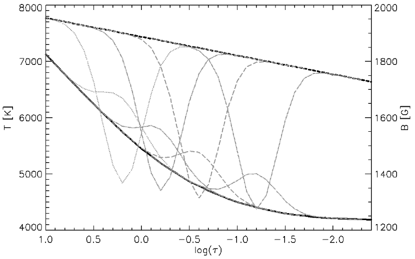
Figure 3: The background stratifications of temperature (solid black line) and magnetic field strength (dashed black line). The various styles of gray lines represents the gaussian perturbations added to the stratifications of the background model of atmosphere at four different heights.

The original SIR code converges to the same resulting model of atmosphere almost independently of the initial model. However, the modified code cannot change the stratifications of plasma parameters independently as the original one since there are ties between the parameters induced by the gaussian perturbation which must have the same width and position for all of them. Therefore, the resulting model of atmosphere depends on the starting one, especially on the initial position of the gaussian perturbation. The Stokes profiles observed in the analysed region are fitted using four different starting positions for the gaussian perturbation (see figure 3). The merit functions of the resulting models of atmosphere are compared at each pixel and the best solution is used to create maps of plasma parameters.

The starting positions of the gaussian perturbations are $\log(\tau)=0.2\textrm{,}-0.2\textrm{,}-0.6\textrm{, and}-1.2$. Except for the height of the gaussians, the other parameters of the initial guess models are the same: HWHM, $\sigma$, of the gaussian function is 0.5 in units of the logarithm of optical depth, the amplitude of the perturbation is $+$800 K for the temperature, $-500$ G for the magnetic field strength, $+$3 km s^-1 for the line-of-sight velocity, $-30^{\circ}$ for the field inclination, and $-5^{\circ}$ for the field azimuth. The background stratifications are the same in all four cases. In total, the inversion retrieves 13 free parameters.

The initial amplitudes of the gaussian perturbation have been chosen on the basis of two-component inversions of the penumbral fine structure (e.g. Bellot Rubio et al., 2004; Borrero et al., 2006) and because such perturbations can represent currently available theoretical models of the penumbra: the moving flux tube model (Schlichenmaier et al., 1998) and the field-free gap model (Scharmer & Spruit, 2006). These two models have similar characteristics from an observational point of view, that is, weaker and rather horizontal fields embedded in a strong and less inclined background field. The moving flux tube model predicts that the weak fields are associated with increased velocities. Gaussian perturbations with initial amplitudes such as the ones used here can simulate the top of field-free gaps or low-lying penumbral flux tubes if they are positioned around the continuum forming layer ($\log(\tau)=0.2$ or $-0.2$), or penumbral flux tubes if they are located higher in the line forming region.

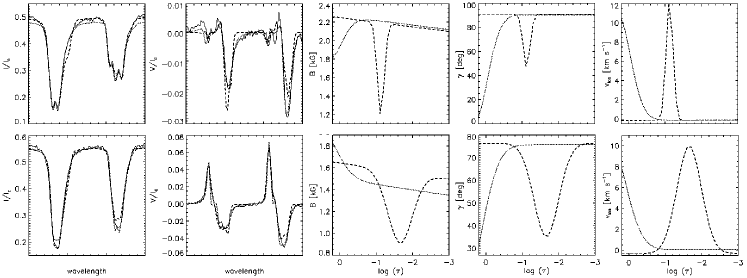
Figure 4: Observed Stokes $I$ and $V$ profiles (solid lines) plotted together with the synthetic profiles and stratifications of magnetic field strength, inclination, and LOS velocity obtained using the SIR/GAUSS code with starting position of the gaussian perturbation at $\log(\tau)=0.2$ (dotted lines) and $\log(\tau)=-1.2$ (dashed lines). The upper row shows an example of the profiles observed in the inner penumbra, where the mid penumbra is represented by the profiles displayed in the lower row.

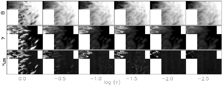
Figure 5: Resulting maps of magnetic field strength, inclination, and LOS velocity (from top to bottom) at different heights in the atmosphere. The colour codes for displayed plasma parameters are the same as in figure 6, see the colour bars there.

4 Penumbral Fine Structure

As only a small part of the penumbra is analysed and the studied area does not cover the whole width of the penumbra, no general conclusions about the penumbral structure are made here. We selected this region because lots of clearly defined bright filaments enter the umbra, enabling us to study their plasma properties with high precision using the method described above. Moreover, the Stokes $V$ profiles observed in the limb-side penumbra at a given position on the solar disc are highly asymmetric. The asymmetries can be explained only with gradients of velocity and magnetic field in the line forming region and thus the presence of gaussian perturbations in the stratifications of these plasma parameters is necessary because the gradients in the background component are too small to produce such asymmetric profiles.

Figure 4 shows two examples of observed profiles. The upper row displays Stokes $I$ and $V$ profiles observed in the inner penumbra (solid lines) together with the synthetic profiles and stratifications of magnetic field strength, inclination, and LOS velocity obtained using the SIR/GAUSS code with starting position of the gaussian perturbation at $\log(\tau)=0.2$ (dotted lines) and $\log(\tau)=-1.2$ (dashed lines). The same applies for the lower row, where a pixel from the mid penumbra is studied.

The inclination is evaluated with respect to the line of sight in these plots. We can see that the inclination of the background field is in both cases close to $90^{\circ}$ and thus the $V$ profiles generated by this component are weak. In the inner penumbra the background component has opposite polarity with respect to the gaussian component (it is slightly larger than $90^{\circ}$) and that together with the velocity difference are the main reasons for the asymmetric $V$ profile. The polarity of the background and gaussian components are the same in the mid penumbra, therefore we do not see any $V$ lobe cancellation and the asymmetry is caused only by the difference in LOS velocities.

The solution in the inner penumbra is easy to interpret as the best fits are always obtained using gaussian perturbation deep in the atmosphere. In the example shown in the upper row of figure 4, the merit function is $12.3$ for the solution obtained with gaussian perturbation low in the atmosphere compared to $\chi^{2}=22.6$ for that obtained with the gaussian located higher in the line forming region.

On the other hand, the correct solution in the mid penumbra is much harder to find. In the example of figure 4, the fit obtained using the initial perturbation high in the atmosphere is better ($\chi^{2}$=18.2 for $\log(\tau)=-1.2$ vs. $\chi^{2}$=25.9 for $\log(\tau)=0.2$), although the shown fits to the Stokes $I$ and $V$ profiles look like of a similar quality. Generally, the variations in merit functions obtained with different starting heights for the gaussian perturbations are not significantly different in the mid penumbra and thus it is difficult to decide which solution is closer to reality. Moreover, the fits are generally worse in the mid penumbra, where $\langle\chi^{2}\rangle=33$, than in the inner penumbra, where $\langle\chi^{2}\rangle=19$.

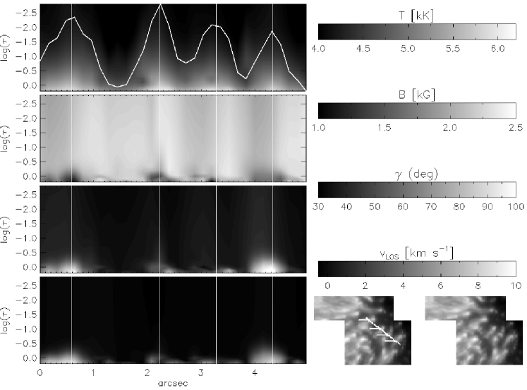
Figure 6: Vertical cut through four bright structures in the inner penumbra is presented. The position of the cut is indicated in the continuum intensity map in the lower left part of the figure. The left part of the figure shows the stratifications of temperature, magnetic field strength, inclination, and LOS velocity (from top to bottom) along this cut, where the right part of the figure displays the colour bars of these plasma parameters. The white line in the temperature stratification map corresponds to the continuum intensity along the cut. The vertical lines in the maps of stratifications correspond to the arrows in the continuum intensity map.

In figure 5 we show the resulting maps of magnetic field strength (upper row), inclination (middle row), and LOS velocity (lower row) at six optical depths. These maps are created from the best solutions which were obtained at each point (selected on the basis of merit function).

This figure clearly shows the discontinuities in the values of plasma parameters in the mid penumbra (upper left part of the analysed region). The problem is that solutions with gaussian perturbation located low and high in the line forming region reproduce the observed Stokes profiles with similar quality and do have different stratifications of plasma parameters (although the resulting stratifications of the background component are similar). At some areas in the mid penumbra we found weaker and more horizontal magnetic field together with increased LOS velocities high in the atmosphere (around $\log(\tau)=-1.5$). A typical example of such a solution is the pixel presented in the lower part of figure 4, dashed line. At other areas the best fit corresponds to the location of the gaussian perturbation low in the atmosphere, i.e. the field is more horizontal and the LOS velocities are increased there. However, for this type of solution the magnetic field strength is either slightly larger or remains basically the same as in the background component (i.e. the amplitude of the gaussian perturbation in field strength is small, see the dotted line in the lower part of figure 4 as an example).

As can be seen, the solution is clear in the inner penumbra, where the best fits correspond to the gaussian perturbation low in the atmosphere. The bright filaments protruding into the umbra have lower magnetic field strengths, more horizontal fields, and significantly larger LOS velocities. Similar conclusions can be made on the basis of figure 6, where the stratifications of various plasma parameters are shown along a cut that cross four bright structures in the inner penumbra (see the caption of this figure for details). In figures 5 and 6, the inclination has been transformed to the local reference frame, i.e. it is measured from the local normal line pointing downwards.

In the case of the magnetic field inclination and LOS velocities, the background stratifications are not significantly influenced by the presence of bright structures and reach similar values as in the surrounding umbra, i.e. the filamentary structure almost disappears higher in the atmosphere. In the case of the stratifications of the magnetic field strength, the filamentary structure is sharpest low in the atmosphere but do not disappear with height. This could be an artefact of the inversion technique, but it remains to be tested.

In the upper map of figure 6 we show the temperature along the cut and the white line representing the continuum intensity along the cut. We can clearly see that the bright structures have naturally higher temperatures low in the atmosphere. The increase of the temperature in such structures is imperative, but the absolute values of the temperature enhancement cannot be always trusted as we occasionally do not fit the continuum of Stokes $I$ profile correctly (mostly because the macro-turbulence, the helping parameter for the line broadening, is set to zero and thus the increase of temperature at lower layers would result into better fit of the continuum intensity but worse fit of the line wings).

Here we make the first rough estimates of the difference between the values of plasma parameters in the bright filaments and the surrounding umbra. The parameters given below correspond to optical depth $\log(\tau)=-0.2$, where the results of the inversion are more reliable than at optical depth unity layer itself. The uncertainties in the plasma parameters will not be discussed here, but are much smaller than the differences we find.

The estimates are made from the bright filaments whose cut is analysed in figure 6. In the case of the magnetic field strength we find a decrease of approximately 600 G (1700 G in the bright filaments compared to 2300 G in the surrounding umbra). This value is similar to those deduced from the two-component inversions performed by Bellot Rubio et al. (2004) and Borrero et al. (2006), i.e. 500 G and 1500 G respectively. In the inner penumbra, these authors found magnetic field inclination around 20^∘ and 60^∘ in the background and the flux-tube component, respectively. The values in the surrounding umbra should be comparable to those of the background atmosphere in two-component inversions, and indeed we find values around 30^∘. However, the field inclinations in bright filaments are around 90^∘ in our case, larger than those derived from two-component inversions. As expected, the LOS velocities are close to zero in the umbra surrounding the bright filaments and reach values around 4 km s^-1 in them. These large velocities are again compatible with the results of Bellot Rubio et al. (2004) and Borrero et al. (2006), who found values of 5 and 3 km s^-1 in the flux-tube component for spots at similar heliocentric angles (40^∘, resp 37^∘). The most important point is that we can directly ascribe these properties to the bright penumbral filaments. That was not possible with the results of the two-component inversions mentioned above.

5 Conclusions

We have introduced a method to analyse the data obtained by SP onboard HINODE using an advanced inversion technique. We have applied this method to the limb-side penumbra of Active Region 10923, observed on November 10, 2006. This allows us to directly obtain the structure of the magnetic field vector together with the velocity configuration of the penumbral fine structure. This is possible for the first time and our preliminary results in the inner penumbra confirm previous results coming from two-component inversions of visible and near-infrared lines. However, inversion techniques have so far been unable to relate the magnetic structures represented by the two components with intensity structures. This had to be done with the help of spectroscopic data or magnetograms which have better spatial resolution.

Using SP data from HINODE SOT, we find that the magnetic field in the bright filaments is weaker by some 600 G compared with the surrounding umbra at optical depth $\log(\tau)=-0.2$. The field is horizontal in those layers and the LOS velocity reaches values around 4 km s^-1. The differences between the plasma parameters in the bright filaments and the surrounding umbra quickly decrease with height and disappear around $\log(\tau)=-0.5$. This means that the bright filaments are structures located deep in the atmosphere in the inner penumbra and that the background magnetic field closes above them. To some extent, such a result is similar to that found in light bridges (Jurčák et al., 2006).

This could support the theory of a field-free gappy penumbra (Scharmer & Spruit, 2006) which hypothesises that bright penumbral filaments and light bridges are the representations of the same phenomena (top of field-free gaps) of different magnitude. However, our results could be also explained by flux tubes located around optical depth unity in the inner penumbra, as predicted by the moving tube model of Schlichenmaier et al. (1998).

The advantage of this model is that strong Evershed flows channeled by the tubes arise naturally from the calculations, whereas the gappy model does not offer any explanation for the Evershed flow. One of the argument against the moving tube model is the large predicted outflow velocity around 13 km s^-1; here we find similar magnitudes of velocities in the mid penumbra. For example 11 km s^-1, if we compute the outflow velocity as $v_{\textrm{\small{LOS}}}/\cos(\gamma_{\textrm{\small{LOS}}})$ and take the value of LOS velocity of 7 km s^-1 and LOS inclination of 50 deg (selected on the basis of the pixel from mid penumbra shown in figure 4, dashed lines, where we do not use the peak values as they are probably overestimated).

The results in the mid penumbra are more difficult to interpret. There are two possible solutions which fit the observed Stokes profiles with similar quality. According to the rising flux tube model, the tubes should be positioned higher in the atmosphere in the outer penumbra and thus a more careful and detailed analysis of this region is needed to test the realism of the two most discussed models of the penumbral fine structure.

This work has been enabled thanks to the funding provided by the Japan Society for the Promotion of Science. Hinode is a Japanese mission developed and launched by ISAS/JAXA, with NAOJ as domestic partner and NASA and STFC (UK) as international partners. It is operated by these agencies in co-operation with ESA and NSC (Norway). The computations were partly carried out at the NAOJ Hinode Science Center, which is supported by the Grant-in-Aid for Creative Scientic Research The Basic Study of Space Weather Prediction from MEXT, Japan (Head Investigator: K. Shibata), generous donations from Sun Microsystems, and NAOJ internal funding.

References

- Beckers & Schröter (1969) Beckers, J. M. & Schröter, E. H. 1969, Sol. Phys., 10, 384
- Bellot Rubio (2003) Bellot Rubio, L. R. 2003, in Astronomical Society of the Pacific Conference Series, Vol. 307, Astronomical Society of the Pacific Conference Series, ed. J. Trujillo-Bueno & J. Sanchez Almeida, 301
- Bellot Rubio et al. (2004) Bellot Rubio, L. R., Balthasar, H., & Collados, M. 2004, A&A, 427, 319
- Bellot Rubio et al. (2005) Bellot Rubio, L. R., Langhans, K., & Schlichenmaier, R. 2005, A&A, 443, L7
- Bellot Rubio et al. (2006) Bellot Rubio, L. R., Schlichenmaier, R., & Tritschler, A. 2006, A&A, 453, 1117
- BellotRubio (2007) BellotRubio, L. R. 2007, in Highlights of Spanish Astrophysics IV, eds. F. Figueras, J.M. Girart, M. Hernanz, and C. Jordi (Springer), in press [astroph/0611471]
- Borrero et al. (2004) Borrero, J. M., Solanki, S. K., Bellot Rubio, L. R., Lagg, A., & Mathew, S. K. 2004, A&A, 422, 1093
- Borrero et al. (2006) Borrero, J. M., Solanki, S. K., Lagg, A., Socas-Navarro, H., & Lites, B. 2006, A&A, 450, 383
- Jurčák et al. (2006) Jurčák, J., Martínez Pillet, V., & Sobotka, M. 2006, A&A, 453, 1079
- Jurčák (2006) Jurčák, J. 2006, Two dimensional spectropolarimetry of a sunspot, doctoral thesis, Charles University, Prague
- Kosugi (2007) Kosugi, T., et al. 2007, Sol. Phys., to be submited
- Langhans et al. (2005) Langhans, K., Scharmer, G. B., Kiselman, D., Löfdahl, M. G., & Berger, T. E. 2005, A&A, 436, 1087
- Ruiz Cobo (1998) Ruiz Cobo, B. 1998, Ap&SS, 263, 331
- Ruiz Cobo & del Toro Iniesta (1992) Ruiz Cobo, B. & del Toro Iniesta, J. C. 1992, ApJ, 398, 375
- Scharmer & Spruit (2006) Scharmer, G. B. & Spruit, H. C. 2006, A&A, 460, 605
- Schlichenmaier et al. (1998) Schlichenmaier, R., Jahn, K., & Schmidt, H. U. 1998, A&A, 337, 897
- Solanki (2003) Solanki, S. K. 2003, A&A Rev., 11, 153
- Tarbell (2007) Tarbell, T., et al. 2007, Sol. Phys., to be submited
- Tsuneta (2007) Tsuneta, S., et al. 2007, Sol. Phys., to be submited