An accurate finite element method for elliptic interface problems

Abstract

A finite element method for elliptic problems with discontinuous coefficients is presented. The discontinuity is assumed to take place along a closed smooth curve. The proposed method allows to deal with meshes that are not adapted to the discontinuity line. The (nonconforming) finite element space is enriched with local basis functions. We prove an optimal convergence rate in the $H^{1}$–norm. Numerical tests confirm the theoretical results.

1 Introduction

Boundary value problems with discontinuous coefficients constitute a prototype of various problems in heat transfer and continuum mechanics where heterogeneous media are involved. The numerical solution of such problems requires much care since their solution does not generally enjoy enough smoothness properties required to obtain optimal convergence rates. Although fitted or adapted meshes can handle such difficulties, these solution strategies become expensive if the discontinuity front evolves with time or within an iterative process. Such a (weak) singularity appears also in the numerical solution of other types of problems like free boundary problems when they are formulated for a fixed mesh or for fictitious domain methods.

We address, in this paper, a new finite element approximation of a model elliptic transmission problem that allows nonfitted meshes. It is well known that the standard finite element approximation of such a problem does not converge with a first order rate in the $H^{1}$-norm in the general case. We propose a method that converges optimally provided the interface curve is a sufficiently smooth curve. Our method is based on a local enrichment of the finite element space in the elements intersected by the interface. The local feature is ensured by the use of a hybrid approximation. A Lagrange multiplier enables to recover the conformity of the approximation. The derived method appears then rather as a local modification of the equations of interface elements than a modification of the linear system of equations. This property ensures that the structure of the matrix of the linear system is not affected by the enrichment.

Let us mention other authors who addressed this topic in the finite element context. We point out the so-called XFEM (eXtended Finite Element Methods) developed in Belytschko et al. [3] where the finite element space is modified in interface elements by using the level set function associated to the interface. Such methods, that are used also for crack propagation, have in our point of view, the drawback of resulting in a variable matrix structure. Moreover, although no theoretical analysis is available, numerical experiments show that they are not optimal in terms of accuracy. Other authors like Hansbo et al. [13, 12], have similar approaches to ours but here also the proposed method seems to modify the matrix structure by enriching the finite element. In Lamichhane–Wohlmuth [16] and Braess–Dahmen [5], a similar Lagrange multiplier approach is used for a mortar finite element formulation of a domain decomposition method. Finally, in a work by Li et al [15], an immersed interface technique, inspired from finite difference schemes, is adapted to the finite element context. Note also that the references where Lagrange multipliers are employed have for these multipliers as supports the edges defining the interface. In our method, the interface supports the added degrees of freedom but the Lagrange multipliers are defined on the edges intersected by the interface and thus serve to compensate the nonconformity of the finite element space rather than enforcing interface conditions, which are being naturally ensured by the variational formulation.

In the following, we use the space $L^{2}(\Omega)$ equipped with the norm $\|\cdot\|_{0,\Omega}$ and the Sobolev spaces $H^{m}(\Omega)$ and $W^{m,p}(\Omega)$ endowed with the norms $\|\cdot\|_{m,\Omega}$ and $\|\cdot\|_{m,p,\Omega}$ respectively. We shall also use the semi-norm $|\cdot|_{1,\Omega}$ of $H^{1}(\Omega)$. Moreover, if $\Omega_{1}$ and $\Omega_{2}$ form a partition of $\Omega$, i.e., $\overline{\Omega}=\overline{\Omega}_{1}\cup\overline{\Omega}_{2}$, $\Omega_{1}\cap\Omega_{2}=\emptyset$ and if $v$ is a function in $W^{m-1,p}(\Omega)$ with $v_{|\Omega_{i}}\in W^{m,p}(\Omega_{i})$, then we shall adopt the convention $v\in W^{m,p}(\Omega_{1}\cup\Omega_{2})$ and denote by $\|v\|_{m,p,\Omega_{1}\cup\Omega_{2}}$ the broken Sobolev norm

$$\|v\|_{m,p,\Omega_{1}\cup\Omega_{2}}=\|v\|_{m-1,p,\Omega}+\|v\|_{m,p,\Omega_{1}}+\|v\|_{m,p,\Omega_{2}}.$$

Similarly, we denote by $\|\cdot\|_{m,\Omega_{1}\cup\Omega_{2}}$ and $|\cdot|_{m,\Omega_{1}\cup\Omega_{2}}$, the broken Sobolev norm and semi-norm respectively for the $H^{m}$–space. Finally, we shall denote by $C$, $C_{1},C_{2},\ldots$ various generic constants that do not depend on mesh parameters and by $|A|$ the Lebesgue measure of a set $A$ and by $A^{\circ}$ the interior of a set $A$.

Let $\Omega$ denote a domain in $\mathbb{R}^{2}$ with smooth boundary $\Gamma$ and let $\gamma$ stand for a closed $C^{2}$-curve in $\Omega$ which separates $\Omega$ into two disjoint subdomains $\Omega^{+}$, $\Omega^{-}$ such that $\Omega=\Omega^{+}\cup\gamma\cup\Omega^{-}$ and $\partial\Omega^{+}=\gamma$. For given $f\in L^{2}(\Omega)$ and $a\in L^{\infty}(\Omega)$ we consider the transmission problem:

$$\left\{\begin{aligned} {}-\nabla\cdot(a\nabla u)&=f&&\qquad\text{in }\Omega^{+}\cup\Omega^{-},\\ u&=0&&\qquad\text{on }\Gamma,\\ [u]=\big{[}a\frac{\partial u}{\partial n}\big{]}&=0&&\qquad\text{on }\gamma,\end{aligned}\right.$$

where $[v]$ denotes the jump of a quantity $v$ across the interface $\gamma$ and $n$ is the normal unit vector to $\gamma$ pointing into $\Omega^{-}$. For definiteness we let $[v]=v^{-}-v^{+}$ with $v^{\pm}=v_{|\Omega^{\pm}}$. In addition to boundedness of the diffusion coefficient we assume

$$\begin{split}a^{\pm}&\in W^{1,\infty}(\Omega^{\pm}),\\ a(x)&\geq\alpha>0,\qquad\text{for }x\in\Omega,\end{split}$$ (1)

i.e. $a$ is uniformly continuous on $\Omega\setminus\gamma$, but discontinuous across $\gamma$.

The standard variational formulation of this problem consists in seeking $u\in H^{1}_{0}(\Omega)$ such that

$$\int_{\Omega}a\,\nabla u\cdot\nabla v\,dx=\int_{\Omega}fv\,dx\qquad\forall\ v\in H^{1}_{0}(\Omega).$$ (2)

In view of the ellipticity condition (1), Problem (2) has a unique solution $u$ in $H^{1}_{0}(\Omega)$ but clearly $u\notin H^{2}(\Omega)$. We shall assume throughout this paper the regularity properties:

$$u_{|\Omega^{-}}\in H^{2}(\Omega^{-}),\quad u_{|\Omega^{+}}\in H^{2}(\Omega^{+}),$$

$$\|u\|_{2,\Omega^{-}\cup\Omega^{+}}\leq C\,\|f\|_{0,\Omega}.$$ (3)

Note that these assumptions are satisfied in the case where $a_{|\Omega^{-}}$ and $a_{|\Omega^{+}}$ are constants (see [14, 18] for instance).

In the following, we describe a fitted finite element method. defined by adding extra unknowns on the interface $\gamma$. It turns out that this method leads to an optimal convergence rate. Although it is well suited for the model problem it seems to be inefficient in more elaborate problems which, for example, involve moving interfaces. To circumvent this difficulty, we define a new method where the added degrees of freedom have local supports and then yield a nonconforming finite element method. We show that the use of a Lagrange multiplier removes this nonconformity and ensures an optimal convergence rate.

2 A fitted finite element method

Assume that the domain $\Omega$ is a convex polygon and consider a regular triangulation ${\mathscr{T}}_{h}$ of $\overline{\Omega}$ with closed triangles whose edges have lengths $\leq h$. We assume that $h$ is small enough so that for each triangle $T\in{\mathscr{T}}_{h}$ only the following cases have to be considered:

1. $T\cap\gamma=\emptyset$.

2. $T\cap\gamma$ is an edge or a vertex of $T$.

3. $\gamma$ intersects two different edges of $T$ in two distinct points different from the vertices.

4. $\gamma$ intersects one edge and its opposite vertex.

Let $V_{h}$ denote the lowest degree finite element space

$$V_{h}=\{\,v\in C^{0}(\overline{\Omega});\ v_{|T}\in P_{1}(T)\ \forall\ T\in{\mathscr{T}}_{h},\ v=0\text{ on }\Gamma\},$$

where $P_{1}(T)$ is the space of affine functions on $T$. A finite element approximation of (2) consists in computing $u_{h}\in V_{h}$ such that

$$\int_{\Omega}a\,\nabla u_{h}\cdot\nabla v\,dx=\int_{\Omega}fv\,dx\qquad\forall\ v\in V_{h}.$$ (4)

It is well known that, since $u\notin H^{2}(\Omega)$, the classical error estimates (see [8]) do not hold any more even though we still have the convergence result,

$$\lim_{h\to 0}\|u-u_{h}\|_{1,\Omega}=0.$$

A fitted treatment of the interface $\gamma$ can however improve this result. Let for this purpose $\mathscr{T}_{h}^{\gamma}$ denote the set of triangles that intersect the interface $\gamma$ corresponding to cases 3) and 4) above,

$$\mathscr{T}_{h}^{\gamma}:=\{T\in\mathscr{T}_{h};\ \gamma\cap T^{\circ}\neq\emptyset\},$$

and consider a continuous piecewise linear interpolation of $\gamma$, denoted by $\gamma_{h}$, as shown in Figure 1. Clearly, $\gamma_{h}$ is the line that intersects $\gamma$ at two edges of any triangle that contains $\gamma$. Unless the intersection of $\gamma$ with the boundary of a triangle $T$ does not coincide with an edge, $T$ is split into two sets $T^{+}$ and $T^{-}$ separated by the curve $\gamma$. In case 3), the straight line $\gamma_{h}\cap T$ splits $T$ into a triangle $K_{1}$ and a quadrilateral that we split into two subtriangles $K_{2}$ and $K_{3}$, where we choose $K_{2}$ such that $K_{1}\cap K_{2}=\gamma_{h}$. In case 4), $\gamma_{h}\cap T$ splits $T$ into two triangles $K_{1}$ and $K_{2}$. In this case we set $K_{3}=\emptyset$. This construction defines the new fitted finite element mesh of the domain $\Omega$ (see Figure 1). The splitting $T=K_{1}\cup K_{2}\cup K_{3}$ is not unique but the convergence analysis does not depend on it. Let us denote by $\mathscr{T}_{T}^{\gamma}$ the set of the three subtriangles of $T$. Below $\mathscr{E}_{h}$ will stand for the set of all edges of elements and $\mathscr{E}_{h}^{\gamma}$ is the set of all edges that are intersected by $\gamma$ (or $\gamma_{h}$), i.e.

$$\mathscr{E}_{h}^{\gamma}:=\{e\in\mathscr{E}_{h};\ \gamma\cap e^{\circ}\neq\emptyset\}.$$

For each $T\in\mathscr{T}_{h}$, $\mathscr{E}_{T}$ is the set of the three edges of $T$.

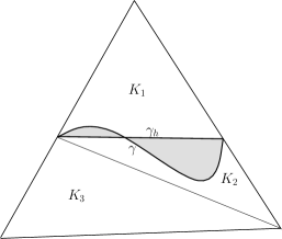
Fig. 1: Subdivision of interface triangles.

The fitted mesh is denoted by $\mathscr{T}_{h}^{F}$, i.e.

$$\mathscr{T}_{h}^{F}:=\mathscr{T}_{h}\cup\bigcup_{T\in\mathscr{T}_{h}^{\gamma}}\Big{(}\cup_{K\in\mathscr{T}_{K}^{\gamma}}K\Big{)}.$$

and by $S_{h}^{\gamma}:=\bigcup\{T;\ T\in\mathscr{T}_{h}^{\gamma}\}$. Let us finally note that the curve $\gamma_{h}$ defines a new splitting of $\Omega$ into two subdomains $\Omega^{-}_{h}$ and $\Omega^{+}_{h}$ where $\Omega^{\pm}_{h}$ is defined analogously to $\Omega^{\pm}$ with $\gamma$ replaced by $\gamma_{h}$.

Next we construct an approximation of the function $a$ on the elements of $\mathscr{T}_{h}^{F}$: For this purpose, let $\tilde{a}^{\pm}$ be extensions of $a^{\pm}$ to $\Omega$ such that $\tilde{a}^{\pm}\in W^{1,\infty}(\Omega)$. Such extensions exist due to the regularity of $\gamma$ (see [1]). Define $\tilde{a}_{h}\in W^{1,\infty}(\Omega)$ by

$$\tilde{a}_{h}=\begin{cases}\tilde{a}^{+}&\text{in }\Omega_{h}^{+},\\ \tilde{a}^{-}&\text{in }\Omega_{h}^{-},\end{cases}$$

and denote by $a_{h}$ the piecewise linear interpolant of $\tilde{a}$ on $\mathscr{T}_{h}^{F}$. Hence $a_{h}$ is continuous on $\Omega_{h}^{+}\cup\Omega_{h}^{-}$ and coincides with $a$ on the nodes of $\mathscr{T}_{h}^{F}$. In addition, the function $a_{h}$ is discontinuous across the line $\gamma_{h}$ and satisfies the properties,

$$a_{h|\Omega^{+}_{h}}\in W^{1,\infty}(\Omega^{+}_{h}),\ a_{h|\Omega^{-}_{h}}\in W^{1,\infty}(\Omega^{-}_{h}),$$ (5)

$$\|a_{h}\|_{0,\infty,\Omega}\leq C\,\|a\|_{0,\infty,\Omega},$$ (6)

$$a_{h}\geq\alpha>0\qquad\text{a.e. in }\Omega.$$ (7)

We now define the finite element space

$$W_{h}=V_{h}+X_{h},$$

$$X_{h}:=\{v\in C^{0}(\overline{\Omega});\ v_{|\Omega\setminus S_{h}^{\gamma}}=0,\ v_{|K}\in P_{1}(K)\ \forall\ K\in\mathscr{T}_{T}^{\gamma},\ \forall\ T\in\mathscr{T}_{h}^{\gamma}\}.$$

Note that we have $W_{h}\subset H^{1}_{0}(\Omega)$. A fitted finite element approximation is defined as the follows:

$$\left\{\begin{aligned} {}&\text{Find }u_{h}^{F}\in W_{h}\text{ such that}\\ &\int_{\Omega}a_{h}\nabla u_{h}^{F}\cdot\nabla v\,dx=\int_{\Omega}fv\,dx\qquad\forall\ v\in W_{h}.\end{aligned}\right.$$ (8)

In order to study the convergence of Problem (8), we consider the auxiliary problem:

$$\left\{\begin{aligned} {}&\text{Find }\widehat{u}_{h}\in H^{1}_{0}(\Omega)\text{ such that}\\ &\int_{\Omega}a_{h}\nabla\widehat{u}_{h}\cdot\nabla v\,dx=\int_{\Omega}fv\,dx\qquad\forall\ v\in H^{1}_{0}(\Omega).\end{aligned}\right.$$ (9)

We note that both problems (8) as well as (9) have a unique solution. The regularity properties (3) imply $u^{+}\in C^{0}(\bar{\Omega}^{+})$, $u^{-}\in C^{0}(\bar{\Omega}^{-})$ and that $u^{+}$ and $u^{-}$ have a common trace on $\gamma$. Therefore $u$ is continuous on $\Omega$ and the piecewise $P_{1}$ interpolant $I_{h}u\in W_{h}$ is well defined. In the following let $\tilde{u}^{\pm}\in H^{2}(\Omega)$ stand for the extensions of $u^{\pm}$ from $\Omega^{\pm}$ to $\Omega$.

In the sequel, we assume that the fitted family of meshes $(\mathscr{T}_{h}\cup\mathscr{T}_{h}^{\gamma})_{h}$ satisfies the condition

$$\frac{h}{\varrho}\leq C\,h^{-\theta}$$ (10)

for some $\theta\in[0,1)$ and for which $C$ is independent of $h$, where $\varrho$ denotes the radius of the largest ball contained in any triangle in any triangle $T\in\mathscr{T}_{h}^{F}$.

Lemma 2.1.

Let $u\in H^{2}(\Omega^{+}\cup\Omega^{-})$.

1. We have the local interpolation error

   $$|u-I_{h}u|_{1,T}\leq\begin{cases}Ch\,|u|_{2,T}&\text{for }T\in\mathscr{T}_{h}\setminus\mathscr{T}_{h}^{\gamma}\\ C\frac{h^{2}}{\varrho_{K}}(|\tilde{u}^{+}|_{2,K}+|\tilde{u}^{-}|_{2,K})&\text{for }K\in\mathscr{T}_{T}^{\gamma},\,T\in\mathscr{T}_{h}^{\gamma},\end{cases}$$ (11)

   where $\varrho_{K}$ is the radius of the inscribed circle of $K$.

2. The global interpolation error is given by

   $$|u-I_{h}u|_{1,\Omega}\leq C\,h^{1-\theta}\,|u|_{2,\Omega^{+}\cup\Omega^{-}}.$$ (12)

   Moreover, if $u\in W^{2,\infty}(\Omega^{+}\cup\Omega^{-})$ then

   $$|u-I_{h}u|_{1,\Omega}\leq C\,h\,|u|_{2,\infty,\Omega^{+}\cup\Omega^{-}}.$$ (13)

Proof.

Since the local interpolation error estimate for $T\in\mathscr{T}_{h}\setminus\mathscr{T}_{h}^{\gamma}$ is classic in finite element theory (see [6] or [8] for instance), we only need to prove the second estimate on triangles where $u$ is only piecewise smooth. Consider an element $T\in\mathscr{T}_{h}^{\gamma}$ and any subtriangle $K\in\mathscr{T}_{T}^{\gamma}$. Without loss of generality we assume $K\subset\Omega_{h}^{+}$, then

$$K =(K\cap\Omega^{+})\,\cup\,(K\cap\Omega^{-}).$$

Since $K\cap\Omega^{-}\subset T\cap\Omega^{-}\cap\Omega_{h}^{+}$ and $\gamma_{h}$ interpolates the interface $\gamma$ we obtain for the measure of $K\cap\Omega^{-}$

$$|K\cap\Omega^{-}|\leq|T\cap\Omega^{-}\cap\Omega_{h}^{+}|\leq Ch^{3},$$ (14)

with a constant $C>0$ which depends on $\gamma$ only. In view of $I_{h}u=I_{h}\tilde{u}^{+}$, the standard interpolation theory (see [8] or [6]) implies

$$\begin{split}|u-I_{h}u|_{1,K}&\leq|u-\tilde{u}^{+}|_{1,K}+|\tilde{u}^{+}-I_{h}\tilde{u}^{+}|_{1,K}\\ &\leq|u-\tilde{u}^{+}|_{1,K}+C\,\frac{h^{2}}{\varrho_{K}}\,|\tilde{u}^{+}|_{2,K}.\end{split}$$ (15)

Since $\tilde{u}^{+}=u$ holds on $K\cap\Omega^{+}$ we obtain

$$|u-\tilde{u}^{+}|_{1,K}=|u-\tilde{u}^{+}|_{1,K\cap\,\Omega^{-}}\leq|u^{-}|_{1,K\cap\,\Omega^{-}}+|\tilde{u}^{+}|_{1,K\cap\,\Omega^{-}}.$$

Applying Hölder’s inequality with $p=\frac{3}{2}$ and $q=3$, the imbedding of $H^{1}(K)$ into $L^{6}(K)$ (Note that the imbedding constant can be bounded independently of $h$) and (14) one can bound $|u^{-}|_{1,K\cap\,\Omega^{-}}$ (and analogously $|\tilde{u}^{+}|_{1,K\cap\,\Omega^{-}}$) by

$$|u^{-}|_{1,K\cap\,\Omega^{-}} \leq|K\cap\Omega^{-}|^{\frac{1}{3}}\|\nabla u^{-}\|_{0,6,K\cap\,\Omega^{-}}$$

$$\leq C\,h\,\|\nabla\tilde{u}^{-}\|_{0,6,K}\leq C\,h\,|\tilde{u}^{-}|_{2,K}.$$

Hence

$$|u-\tilde{u}^{+}|_{1,K} \leq C\,h\,(|\tilde{u}^{-}|_{2,K}+|\tilde{u}^{+}|_{2,K}).$$

Inserting this estimate into (15) leads to

$$|u-I_{h}u|_{1,K}\leq C\frac{h^{2}}{\varrho_{K}}\,(|\tilde{u}^{-}|_{2,K}+|\tilde{u}^{+}|_{2,K}).$$

To prove the global interpolation error bound, we write

$$|u-I_{h}u|_{1,\Omega}^{2} =\sum_{T\in\mathscr{T}_{h}\setminus\mathscr{T}_{h}^{\gamma}}|u-I_{h}u|_{1,T}^{2}+\sum_{T\in\mathscr{T}_{h}^{\gamma}}\sum_{K\in\mathscr{T}_{T}^{\gamma}}|u-I_{h}u|_{1,K}^{2}$$

$$\leq Ch^{2}\sum_{T\in\mathscr{T}_{h}\setminus\mathscr{T}_{h}^{\gamma}}|u|^{2}_{2,T}+C\sum_{T\in\mathscr{T}_{h}^{\gamma}}\sum_{K\in\mathscr{T}_{T}^{\gamma}}\frac{h^{2}}{\varrho_{K}}(|\tilde{u}^{-}|^{2}_{2,K}+|\tilde{u}^{+}|^{2}_{2,K})$$

$$\leq C\frac{h^{2}}{\varrho}\,(|\tilde{u}^{-}|^{2}_{2,\Omega}+|\tilde{u}^{+}|^{2}_{2,\Omega})$$

$$\leq C\frac{h^{2}}{\varrho}\,|u|^{2}_{2,\Omega^{+}\cup\,\Omega^{-}},$$

where

$$\varrho =\min\{\varrho_{K}\colon K\in\mathscr{T}_{T}^{\gamma},T\in\mathscr{T}_{h}^{\gamma}\}.$$

The calculation above indicates how the convergence rate can be improved in case $u\in W^{2,\infty}(\Omega^{+}\cup\Omega^{-})$ observing that $|S_{h}^{\gamma}|\leq Ch$ holds. ∎

Remark 2.1.

It is classic in finite element theory to assume that the meshes are regular in the sense that Condition (10) is satisfied for $\theta=0$. For the fitted meshes $\mathscr{T}_{h}^{\gamma}$ one cannot guarantee that such a condition is satisfied. To relax this constraint, we assume here (10) for a $\theta\in[0,1)$ thus allowing a larger class of fitted meshes than permitted by $\theta=0$.

The following result gives the convergence rate for Problem (8).

Theorem 2.1.

Assume that the family of fitted meshes $(\mathscr{T}_{h}^{F})_{h}$ satisfies the regularity property (10). Then we have the error estimate

$$|u-u_{h}^{F}|_{1,\Omega}\leq\begin{cases}Ch^{1-\theta}\,\|u\|_{2,\Omega^{+}\cup\,\Omega^{-}}&\text{if }u\in H^{2}(\Omega^{+}\cup\Omega^{-}),\\ Ch\,\|u\|_{2,\infty,\Omega^{+}\cup\,\Omega^{-}}&\text{if }u\in W^{2,\infty}(\Omega^{+}\cup\Omega^{-}).\end{cases}$$ (16)

Proof.

We have from the triangle inequality

$$|u-u_{h}^{F}|_{1,\Omega}\leq|u-\widehat{u}_{h}|_{1,\Omega}+|\widehat{u}_{h}-u_{h}^{F}|_{1,\Omega}.$$ (17)

To bound the first term on the right-hand side of (17), we proceed as follows: Let us subtract (9) from (2) and choose $v=u-\widehat{u}_{h}$. We have

$$\int_{\Omega}(a\,\nabla u-a_{h}\nabla\widehat{u}_{h})\cdot\nabla(u-\widehat{u}_{h})\,dx=0.$$

Then

$$\int_{\Omega} a_{h}|\nabla(u-\widehat{u}_{h})|^{2}\,dx=-\int_{\Omega}(a-a_{h})\,\nabla u\cdot\nabla(u-\widehat{u}_{h})\,dx$$

$$=-\int_{\Omega\setminus S_{h}^{\gamma}}(a-a_{h})\,\nabla u\cdot\nabla(u-\widehat{u}_{h})\,dx-\sum_{T\in\mathscr{T}_{h}^{\gamma}}\int_{T}(a-a_{h})\,\nabla u\cdot\nabla(u-\widehat{u}_{h})\,dx.$$

The usual estimate for the interpolation error gives

$$\|a-a_{h}\|_{0,\infty,\Omega} \leq Ch\,(\|\tilde{a}\|_{1,\infty,\Omega^{+}_{h}}+\|\tilde{a}\|_{1,\infty,\Omega^{-}_{h}})$$

$$\leq Ch\,\|a\|_{1,\infty,\Omega^{+}\cup\Omega^{-}}.$$

with a constant $C$ which only depends on a reference triangle, (see [8], p. 124). Thus we obtain

$$\bigg{|}\int_{\Omega\setminus S_{h}^{\gamma}}(a-a_{h})\,\nabla u\cdot\nabla(u-\widehat{u}_{h})\,dx\bigg{|}\leq C\,h\,\|a\|_{1,\infty,\Omega^{+}\cup\Omega^{-}}\,|u|_{1,\Omega\setminus S_{h}^{\gamma}}\,|u-\widehat{u}_{h}|_{1,\Omega\setminus S_{h}^{\gamma}}.$$ (18)

Next we consider a triangle $T\in\mathscr{T}_{h}^{\gamma}$ which we split as

$$T=(T\cap\Omega^{+}\cap\Omega_{h}^{+})\cup(T\cap\Omega^{-}\cap\Omega_{h}^{-})\cup(T\cap\Omega^{+}\cap\Omega_{h}^{-})\cup(T\cap\Omega^{-}\cap\Omega_{h}^{+}).$$

As before, we obtain

$$\bigg{|}\int_{T\cap\Omega^{+}\cap\Omega_{h}^{+}}(a-a_{h})\,\nabla u\cdot\nabla(u-\widehat{u}_{h})\,dx\bigg{|}\leq Ch\,\|a\|_{1,\infty,\Omega^{+}\cup\Omega^{-}}|u|_{1,T\cap\Omega^{+}\cap\Omega_{h}^{+}}\,|u-\widehat{u}_{h}|_{1,T\cap\Omega^{+}\cap\Omega_{h}^{+}}.$$

Arguing as in the proof of Lemma 2.1, the generalized Hölder inequality together with (14) yields the estimate

$$\bigg{|}\int_{T\cap\Omega^{+}\cap\Omega_{h}^{-}} (a-a_{h})\,\nabla u\cdot\nabla(u-\widehat{u}_{h})\,dx\bigg{|}$$

$$=\bigg{|}\int_{T\cap\Omega^{+}\cap\Omega_{h}^{-}}(a^{+}-a_{h}^{-})\nabla u^{+}\cdot\nabla(u^{+}-\widehat{u}_{h})\,dx\bigg{|}$$

$$\leq C\,\|a\|_{0,\infty,\Omega}\,|T\cap\Omega^{+}\cap\Omega_{h}^{-}|^{1/3}\,\|\nabla u^{+}\|_{0,6,T\cap\Omega^{+}\cap\Omega_{h}^{-}}\,\|\nabla(u^{+}-\widehat{u}_{h})\|_{0,T\cap\Omega^{+}\cap\Omega_{h}^{-}}$$

$$\leq C\,h\,\|a\|_{0,\infty,\Omega}\,|\tilde{u}^{+}|_{2,T}\,\|\nabla(u^{+}-\widehat{u}_{h})\|_{0,T}.$$

Analogous estimates hold with $+$ and $-$ interchanged. Collecting the four contributions to the triangle $T$ one obtains

$$\bigg{|}\int_{T} (a-a_{h})\,\nabla u\cdot\nabla(u-\widehat{u}_{h})\,dx\bigg{|}$$

$$\leq Ch\,(\|a\|_{0,\infty,\Omega}+\|a\|_{1,\infty,\Omega^{+}\cup\,\Omega^{-}})$$

$$\quad\times\big{(}|\tilde{u}^{+}|_{2,T}\,\|\nabla(u^{+}-\widehat{u}_{h})\,\|_{0,T\cap\Omega^{+}}+|\tilde{u}^{-}|_{2,T}\,\|\nabla(u^{-}-\widehat{u}_{h})\|_{0,T\cap\Omega^{-}}\big{)}.$$

Combining this estimate with (18) leads to

$$\int_{\Omega} a_{h}\,|\nabla(u-\widehat{u}_{h})|^{2}\,dx\leq Ch\,\|a\|_{1,\infty,\Omega^{+}\cup\,\Omega^{-}}|u|_{1,\Omega\setminus S_{h}^{\gamma}}|u-\widehat{u}_{h}|_{1,\Omega\setminus S_{h}^{\gamma}}$$

$$+C\,h\,(\|a\|_{0,\infty,\Omega}+\|a\|_{1,\infty,\Omega^{+}\cup\,\Omega^{-}})$$

$$\quad\times\sum_{T\in\mathscr{T}_{h}^{\gamma}}\Big{(}|\tilde{u}^{+}|_{2,T}\|\nabla(u^{+}-\widehat{u}_{h})\|_{0,T\cap\Omega^{+}}+|\tilde{u}^{-}|_{2,T}\|\nabla(u^{-}-\widehat{u}_{h})\|_{0,T\cap\Omega^{-}}\Big{)}$$

$$\leq C\,h\,\|a\|_{1,\infty,\Omega^{+}\cup\,\Omega^{-}}\,|u|_{1,\Omega\setminus S_{h}^{\gamma}}\,|u-\widehat{u}_{h}|_{1,\Omega\setminus S_{h}^{\gamma}}$$

$$\qquad+C\,h\,(\|a\|_{0,\infty,\Omega}+\|a\|_{1,\infty,\Omega^{+}\cup\,\Omega^{-}})(|\tilde{u}^{+}|_{2,S_{h}^{\gamma}}+|\tilde{u}^{-}|_{2,S_{h}^{\gamma}})\,\|\nabla(u-\widehat{u}_{h})\|_{0,S_{h}^{\gamma}}$$

$$\leq C\,h\,(\|a\|_{0,\infty,\Omega}+\|a\|_{1,\infty,\Omega^{+}\cup\,\Omega^{-}})\,|u|_{2,\Omega^{+}\cup\,\Omega^{-}}\|\nabla(u-\widehat{u}_{h})\|_{0,\Omega},$$

which by (7) implies

$$|u-\widehat{u}_{h}|_{1,\Omega}\leq C\,h\,(\|a\|_{0,\infty,\Omega}+\|a\|_{1,\infty,\Omega^{+}\cup\,\Omega^{-}})\,|u|_{2,\Omega^{+}\cup\,\Omega^{-}}.$$ (19)

To bound the norm $|\widehat{u}_{h}-u_{h}^{F}|_{1,\Omega}$, we have from problems (9) and (8),

$$\int_{\Omega}a_{h}\nabla(\widehat{u}_{h}-u_{h}^{F})\cdot\nabla v\,dx=0\qquad\forall\ v\in W_{h}.$$

Standard finite element approximation theory combined with (5)–(6) gives

$$|\widehat{u}_{h}-u_{h}^{F}|_{1,\Omega}\leq C\,\inf_{v\in W_{h}}|\widehat{u}_{h}-v|_{1,\Omega},$$ (20)

which together with (19) implies

$$|\widehat{u}_{h}-u_{h}^{F}|_{1,\Omega} \leq C\,|\widehat{u}_{h}-I_{h}u|_{1,\Omega}$$

$$\leq C\,|\widehat{u}_{h}-u|_{1,\Omega}+C\,|u-I_{h}u|_{1,\Omega}$$

$$\leq C\,h\,|u|_{2,\Omega^{+}\cup\,\Omega^{-}}+C\,|u-I_{h}u|_{1,\Omega}.$$

The interpolation error is bounded using (12) or (13). ∎

3 A hybrid approximation

The method presented in the previous section has proven its efficiency as numerical tests will show in the last section. In more elaborate problems like time dependent or nonlinear problems where the interface $\gamma$ is a moving front, the subtriangulation $\mathscr{T}_{h}^{\gamma}$ moves within iterations and then the matrix structure has to be frequently modified. To remedy to this difficulty, we resort to a hybridization of the added unknowns. More specifically, the added discrete space $X_{h}$ is replaced by a nonconforming approximation space. In addition, a Lagrange multiplier is used to compensate this inconsistency. The hybridization enables to locally eliminate the added unknowns in each triangle $T\in\mathscr{T}_{h}^{\gamma}$. In the sequel we fix an orientation for the interface $\gamma$. This induces an orientation of the normals to the edges $e\in\mathscr{E}_{h}^{\gamma}$ by following the interface in the positive direction. The jump of a function $v$ across an edge $e\in\mathscr{E}_{h}^{\gamma}$ can then be defined as

$$[v]_{e}(x):=\lim_{s\to 0,s>0}v(x+sn(x))-\lim_{s\to 0,s<0}v(x+sn(x))\equiv v^{+}(x)-v^{-}(x),\qquad x\in e,$$

where $n$ is the unit normal to $e$.

To develop this method, we start by defining an ad-hoc formulation for the solution $\widehat{u}_{h}$ of (9). Let us define the spaces

$$\widehat{Z}_{h} :=H^{1}_{0}(\Omega)+\widehat{Y}_{h},$$

$$\widehat{Y}_{h} :=\{v\in L^{2}(\Omega);\ v_{|\Omega\setminus S_{h}^{\gamma}}=0,\ v_{|T}\in H^{1}(T)\ \forall\ T\in\mathscr{T}_{h}^{\gamma},$$

$$\qquad[v]=0\text{ on }e,\ \forall\ e\in\mathscr{E}_{h}\setminus\mathscr{E}_{h}^{\gamma}\},$$

$$\widehat{Q}_{h} :=\prod_{e\in\mathscr{E}_{h}^{\gamma}}H^{-\frac{1}{2}}_{00}(e),$$

where $H^{-\frac{1}{2}}_{00}(e)$ is the dual space of the trace space

$$H^{\frac{1}{2}}_{00}(e):=\{v_{|e};\ v\in H^{1}(T),\ e\in\mathscr{E}_{T},\ v=0\text{ on }d\quad\forall\ d\in\mathscr{E}_{T},d\neq e\}.$$

We remark that the jumps $[v]$ for $v\in\widehat{Z}_{h}$ can be interpreted in $H^{\frac{1}{2}}_{00}(e)$ for $e\in\mathscr{E}_{h}^{\gamma}$. This is due to the fact that $v\in H^{1}(T)$ for all $T\in\mathscr{T}_{h}$, that for every $e\in\mathscr{E}_{h}^{\gamma}$, the jump of $v$ lies in $H^{\frac{1}{2}}(e)$ and vanishes at the endpoints of $e$ as well as on at least two adjacent edges. This motivates the choice of $\widehat{Q}_{h}$.

The elements of $\widehat{Q}_{h}$ will be referred to by $\mu=(\mu_{e})_{e\in\mathscr{E}_{h}^{\gamma}}$. We endow $\widehat{Z}_{h}$ with the broken norm

$$\|u\|_{\widehat{Z}_{h}}=(\sum_{T\in\mathscr{T}_{h}}|u|^{2}_{1,T})^{1/2}.$$

On $\widehat{Q}_{h}$ we use the norm

$$\|\mu\|_{\widehat{Q}_{h}}=\Big{(}\sum_{e\in\mathscr{E}_{h}^{\gamma}}\|\mu_{e}\|^{2}_{H^{-\frac{1}{2}}_{00}(e)}\Big{)}^{\frac{1}{2}}:=\Bigg{(}\sum_{e\in\mathscr{E}_{h}^{\gamma}}\bigg{(}\sup_{v\in H^{\frac{1}{2}}_{00}(e)\setminus\{0\}}\frac{\int_{e}\mu_{e}v\,ds}{\|v\|_{H^{\frac{1}{2}}_{00}(e)}}\bigg{)}^{2}\Bigg{)}^{\frac{1}{2}}.$$

Above, the integrals over edges $e$ are to be interpreted as duality pairings between $H^{-\frac{1}{2}}_{00}(e)$ and $H^{\frac{1}{2}}_{00}(e)$. We mention that the broken norm in $\widehat{Z}_{h}$ reflects the fact that $\widehat{Z}_{h}$ is not a subspace of $H_{0}^{1}(\Omega)$.

Next we define the variational problem,

$$\text{Find }(\widehat{u}_{h}^{H},\widehat{\lambda}_{h})\in\widehat{Z}_{h}\times\widehat{Q}_{h}\text{ such that:}$$

$$\sum_{T\in\mathscr{T}_{h}}\int_{T}a_{h}\,\nabla\widehat{u}_{h}^{H}\cdot\nabla v\,dx-\sum_{e\in\mathscr{E}_{h}^{\gamma}}\int_{e}\widehat{\lambda}_{h}\,[v]\,ds=\int_{\Omega}fv\,dx \qquad\forall\ v\in\widehat{Z}_{h},$$ (21)

$$\sum_{e\in\mathscr{E}_{h}^{\gamma}}\int_{e}\mu\,[\widehat{u}_{h}^{H}]\,ds=0 \qquad\forall\ \mu\in\widehat{Q}_{h}.$$ (22)

The saddle point problem (21)–(22) indicates that the continuity of $\widehat{u}_{h}$ across the edges of $\mathscr{E}_{h}^{\gamma}$ is enforced by a Lagrange multiplier technique.

Theorem 3.1.

Problem (21)–(22) has a unique solution $(\widehat{u}_{h}^{H},\widehat{\lambda}_{h})\in\widehat{Z}_{h}\times\widehat{Q}_{h}$. Moreover, we have $\widehat{u}_{h}^{H}=\widehat{u}_{h}$ and the following estimate holds

$$\|\widehat{u}_{h}^{H}\|_{\widehat{Z}_{h}}+\|\widehat{\lambda}_{h}\|_{\widehat{Q}_{h}}\leq C\,\|f\|_{0,\Omega},$$ (23)

with a constant $C$ which is independent of $h$.

Proof.

Problem (21)–(22) can be put in the standard variational form

$$\left\{\begin{aligned} {}&\mathscr{A}(\widehat{u}^{H}_{h},v)+\mathscr{B}(v,\widehat{\lambda}_{h})=(f,v)&&\qquad\forall\ v\in\widehat{Z}_{h},\\ &\mathscr{B}(\widehat{u}^{H}_{h},\mu)=0&&\qquad\forall\ \mu\in\widehat{Q}_{h},\end{aligned}\right.$$

where

$$\mathscr{A}(u,v)=\sum_{T\in\mathscr{T}_{h}}\int_{T}a_{h}\,\nabla u\cdot\nabla v\,dx,$$

$$\mathscr{B}(v,\mu)=-\sum_{e\in\mathscr{E}_{h}^{\gamma}}\int_{e}\mu\,[v]\,ds,$$

$$(f,v)=\int_{\Omega}fv\,dx.$$

The bilinear form $\mathscr{A}$ is clearly continuous and coercive on the space $\widehat{Z}_{h}\times\widehat{Z}_{h}$. The bilinear form $\mathscr{B}$ is also continuous on $\widehat{Z}_{h}\times\widehat{Q}_{h}$.

Next we verify that $\mathscr{B}$ satisfies the inf-sup condition, i.e. there exists $\delta>0$ such that for every $\lambda\in\widehat{Q}_{h}$ there exists $v_{\mu}\in\widehat{Z}_{h}$ such that

$$\mathscr{B}(v_{\mu},\mu)\geq\delta\,\|v_{\mu}\|_{\widehat{Z}_{h}}\|\mu\|_{\widehat{Q}_{h}}$$

i.e.

$$\sum_{e\in\mathscr{E}_{h}^{\gamma}}\int_{e}\mu_{e}[v_{\mu}]\,ds\geq\delta\,\|v_{\mu}\|_{\widehat{Z}_{h}}\|\mu\|_{\widehat{Q}_{h}}$$ (24)

holds.

Given $\mu=(\mu_{e})_{e\in\mathscr{E}^{\gamma}_{h}}\in\widehat{Q}_{h}$ and an edge $e\in\mathscr{E}_{h}^{\gamma}$ choose a triangle $T\in\mathscr{T}_{h}^{\gamma}$ which has $e$ as one of its edges. Define $v_{T}\in H^{1}(T)$ as the solution of

$$\left\{\begin{aligned} {}&\Delta v=0&&\qquad\text{in }T,\\ &\frac{\partial v}{\partial n}=\mu_{e}&&\qquad\text{on }e,\\ &v=0&&\qquad\text{on }\partial T\setminus e,\end{aligned}\right.$$ (25)

which is equivalent to

$$\int_{T}\nabla v\cdot\nabla\varphi\,dx=\int_{e}\mu_{e}\varphi\,ds\quad\text{for }\varphi\in H^{1}_{e}(T)$$

where

$$H^{1}_{e}(T)=\{\varphi\in H^{1}(T);\ \varphi=0\text{ on }\partial T\setminus e\}.$$

By Green’s theorem we obtain

$$\|\mu_{e}\|_{-1/2,e} =\Big{\|}\frac{\partial v_{T}}{\partial n}\Big{\|}_{-1/2,e}\leq\|\nabla v_{T}\|_{0,T},$$

$$\int_{e}\mu_{e}v_{T}\,ds =\int_{T}|\nabla v_{T}|^{2}\,dx,$$

which implies

$$\|\mu_{e}\|_{-1/2,e}^{2}\leq\int_{T}|\nabla v_{T}|^{2}\,dx=\int_{e}\mu_{e}v_{T}\,ds.$$

Let $\chi_{T}$ denote the characteristic function of $T$ and define

$$v_{\mu}=\sum_{T\in\mathscr{T}_{h}^{\Gamma}}\chi_{T}v_{T}.$$

Since there are as many edges in $\mathscr{E}_{h}^{\gamma}$ as triangles in $\mathscr{T}_{h}^{\gamma}$ then $[v_{\mu}]=v_{T}$ holds for every edge $e\in\mathscr{E}_{h}^{\gamma}$. Hence we obtain

$$\|\mu\|^{2}_{\widehat{Q}_{h}}=\sum_{e\in\mathscr{E}_{h}^{\gamma}}\|\mu_{e}\|_{-1/2,e}^{2}\leq\sum_{T\in\mathscr{T}_{h}^{\gamma}}\|\nabla v_{T}\|^{2}_{0,T}=\sum_{e\in\mathscr{E}_{h}^{\gamma}}\int_{e}\mu_{e}[v_{\mu}]\,ds.$$

Furthermore,

$$\|v_{\mu}\|^{2}_{\widehat{Z}_{h}}=\sum_{T\in\mathscr{T}_{h}}\|\nabla v_{T}\|^{2}_{0,T}=\sum_{T\in\mathscr{T}_{h}^{\gamma}}\|\nabla v_{T}\|^{2}_{0,T}$$

holds. This implies

$$\|\mu\|^{2}_{\widehat{Q}_{h}}\|v_{\mu}\|^{2}_{\widehat{Z}_{h}}\leq\Big{(}\sum_{T\in\mathscr{T}_{h}^{\gamma}}\|\nabla v_{T}\|^{2}_{0,T}\Big{)}^{2}=\mathscr{B}(v_{\mu},\mu)^{2}.$$

Adjusting the sign of $v_{\mu}$ this is equivalent to (24) with $\delta=1$. The estimate (23) is a direct consequence of (24).

Now, it is clear from (22) that

$$[\widehat{u}_{h}^{H}]=0\quad\text{on e},\quad\forall\ e\in\mathscr{T}_{h}^{\gamma}.$$

This implies that $\widehat{u}_{h}^{H}\in H^{1}_{0}(\Omega)$. Choosing a test function $v\in H^{1}_{0}(\Omega)$ in (21), we find that $\widehat{u}_{h}^{H}$ is a solution to Problem (9), and then $\widehat{u}^{H}_{h}=\widehat{u}_{h}$. The interpretation of $\widehat{\lambda}_{h}$ is simply obtained by the Green’s formula. ∎

We are now able to present a numerical method to solve the interface problem. This one is simply derived as a finite element method to solve the saddle point problem (21)–(22). We consider for this end a piecewise constant approximation of the Lagrange multiplier. Let us define the finite dimensional spaces,

$$Z_{h} :=V_{h}+Y_{h},$$

$$Y_{h} :=\{v\in L^{2}(\Omega);\ v_{|\Omega\setminus S_{h}^{\gamma}}=0,\ v_{|K}\in P_{1}(K)\ \forall\ K\in\mathscr{T}_{T}^{\gamma},\ \forall\ T\in\mathscr{T}_{h}^{\gamma},$$

$$\qquad[v]=0\text{ on }e,\ \forall\ e\in\mathscr{E}_{h}\setminus\mathscr{E}_{h}^{\gamma}\},$$

$$Q_{h} :=\big{\{}\mu\in\prod_{e\in\mathscr{E}_{h}^{\gamma}}L^{2}(e);\ \mu_{|e}=\text{const.}\quad\forall\ e\in\mathscr{E}_{h}^{\gamma}\big{\}}.$$

The hybrid finite element approximation is given by the following problem:

$$\text{Find }(u^{H}_{h},\lambda_{h})\in Z_{h}\times Q_{h}\text{ such that:}$$

$$\sum_{T\in\mathscr{T}_{h}}\int_{T}a_{h}\,\nabla u^{H}_{h}\cdot\nabla v\,dx-\sum_{e\in\mathscr{E}_{h}^{\gamma}}\int_{e}\lambda_{h}\,[v]\,ds=\int_{\Omega}fv\,dx \qquad\forall\ v\in Z_{h},$$ (26)

$$\sum_{e\in\mathscr{E}_{h}^{\gamma}}\int_{e}\mu\,[u^{H}_{h}]\,ds=0 \qquad\forall\ \mu\in Q_{h}.$$ (27)

Let us give some additional remarks before proving convergence properties of this method.

1. The matrix formulation of the method has the following form

$$\begin{pmatrix}A&C&0\\ C^{T}&D&B\\ 0&B^{T}&0\end{pmatrix}\begin{pmatrix}\widetilde{u}\\ \widetilde{v}\\ \widetilde{\lambda}\end{pmatrix}=\begin{pmatrix}b\\ c\\ 0\end{pmatrix},$$ (28)

where the vector $\widetilde{u}$ contains the values of $u_{h}^{H}$ at nodes of the mesh $\mathscr{T}_{h}$, i.e. components of $u_{h}^{H}$ in the Lagrange basis of $V_{h}$, $\widetilde{v}$ contains the components of $u_{h}^{F}$ in the basis of $Y_{h}$, and $\widetilde{\lambda}$ has as components the values of $\lambda_{h}$ on the edges of $\mathscr{E}_{h}^{\gamma}$. There is clearly no simple method to eliminate off diagonal blocks in the system (28) in order to decouple the variables. More specifically, our aim is to eliminate the unknowns $\widetilde{v}$.

2. The method must be viewed in the context of an iterative process like the Uzawa method, where the Lagrange multiplier $\lambda_{h}$ is decoupled from the primal variable $u_{h}^{H}$. In such situations, each iteration step consists in solving an elliptic problem with a given $\lambda_{h}$. Let us recall that, due to the local feature of the basis functions of nodes on edges of $\mathscr{E}_{h}^{\gamma}$, the unknowns associated to these nodes can be eliminated at the element level. This is a basic issue in our method.

3. We point out that equation (27) entails

$$[u_{h}^{H}]=0\quad\text{on }e,\quad\forall\ e\in\mathscr{T}_{h}^{\gamma}.$$ (29)

This follows from the fact that $u_{h}^{H}$ is an affine function on each edge of $\mathscr{T}_{h}^{\gamma}$. This implies that actually $u_{h}^{H}\in W_{h}$. Choosing $v\in W_{h}$ in (21) we find

$$\int_{\Omega}a_{h}\nabla u_{h}^{H}\cdot\nabla v\,dx=\int_{\Omega}fv\,dx.$$

This yields $u_{h}^{H}=u_{h}^{F}$.

4 Convergence analysis

This section is devoted to the proof of existence, uniqueness and stability of the solution of (26)–(27) as well as its convergence to Problem (21)–(22).

For this result we need a localized quasi-uniformity of the mesh. More precisely, we assume that

$$|e|\geq Ch\qquad\forall\ e\in\mathscr{E}_{h}^{\gamma}.$$ (30)

In addition, we make the following assumption:

The distance of the intersection point of $$\gamma e\in\mathscr{E}_{h}^{\gamma}$$ with any edge (31)

to the endpoints of $$e \delta h \delta$$ can be bounded from below by , where is

independent of $$h$$.

Although this assumption appears to be quite restrictive, numerical tests have shown that it can be actually ignored in applications.

Theorem 4.1.

Assume that the family of meshes $(\mathscr{T}_{h})_{h}$ satisfies Property (30). Then Problem (26)–(27) has a unique solution. Moreover, we have the bound

$$\|u^{H}_{h}\|_{\widehat{Z}_{h}}+\|\lambda_{h}\|_{Q_{h}}\leq C\,\|f\|_{0,\Omega},$$ (32)

where the constant $C$ is independent of $h$.

Proof.

It is clearly sufficient to prove the inf-sup condition (see for instance Brezzi-Fortin [7]):

$$\sup_{v_{h}\in Z_{h}\setminus\{0\}}\dfrac{\sum_{e\in\mathscr{E}_{h}^{\gamma}}\int_{e}\mu_{h}\,[v_{h}]\,ds}{\|v_{h}\|_{\widehat{Z}_{h}}\,\|\mu_{h}\|_{\widehat{Q}_{h}}}\geq\beta>0\qquad\forall\ \mu_{h}\in Q_{h}.$$ (33)

In the following, for each triangle $T\in\mathscr{T}_{h}^{\gamma}$, we shall denote by $e^{+}_{T}$ (resp. $e^{-}_{T}$) the edge where $\gamma$ enters $T$ (resp. leaves $T$), and by $\tilde{e}_{T}$ the remaining edge of $T$ (see Figure (2)). Recall that we fixed an orientation for $\gamma$.

Fig. 2: Definition of $e^{+}_{T}$, $e^{-}_{T}$, and $\tilde{e}_{T}$.

Let $\mu_{h}\in Q_{h}$, and let $v\in\widehat{Z}_{h}$ be the function given by Problem (25).

We define a function $v_{h}\in Z_{h}$ by

$$\left\{\begin{aligned} {}&v_{h|T}=0&&\qquad\forall\ T\in\mathscr{T}_{h}\setminus\mathscr{T}_{h}^{\gamma},\\ &\int_{e}v_{h}\,ds=\int_{e}v\,ds&&\qquad\forall\ e\in\mathscr{E}_{T},\ \forall\ T\in\mathscr{T}_{h}^{\gamma}.\end{aligned}\right.$$ (34)

The gradient of $v_{h}$ can be expressed in $T\in\mathscr{T}_{h}^{\gamma}$ by

$$\nabla v_{h|T}=\frac{2}{|e^{-}_{T}|}\bigg{(}\int_{e^{-}_{T}}v\,ds\bigg{)}\,\nabla\varphi_{e^{-}_{T}}+\frac{2}{|e^{+}_{T}|}\bigg{(}\int_{e^{+}_{T}}v\,ds\bigg{)}\,\nabla\varphi_{e^{+}_{T}},$$

where $\varphi_{e^{+}_{T}}$ (resp. $\varphi_{e^{-}_{T}}$) is the basis function of $Z_{h}$ associated to the added node on $e^{+}_{T}$ (resp. $e^{-}_{T}$). Then by using (30) and the Cauchy-Schwarz inequality, we get for each $T\in\mathscr{T}_{h}^{\gamma}$,

$$\|\nabla v_{h}\|_{0,T} =C_{1}\,h^{-1}\bigg{|}\int_{e^{-}_{T}}v\,ds\bigg{|}\,\|\nabla\varphi_{e^{-}_{T}}\|_{0,T}+C_{2}\,h^{-1}\bigg{|}\int_{e^{+}_{T}}v\,ds\bigg{|}\,\|\nabla\varphi_{e^{+}_{T}}\|_{0,T}$$

$$\leq C_{3}\,h^{-\frac{1}{2}}\,\big{(}\|v\|_{0,e_{T}^{-}}\|\nabla\varphi_{e^{-}_{T}}\|_{0,T}+\|v\|_{0,e_{T}^{+}}\,\|\nabla\varphi_{e^{+}_{T}}\|_{0,T}\big{)}.$$ (35)

The trace inequality (see [2], eq. (2.5)) and the Poincaré inequality owing to $v=0$ on $\tilde{e}_{T}$, yield for $T\in\mathscr{T}_{h}^{\gamma}$,

$$\|v\|_{0,e^{\pm}_{T}}\leq C_{4}\,\big{(}h^{-\frac{1}{2}}\|v\|_{0,T}+h^{\frac{1}{2}}\|\nabla v\|_{0,T}\big{)}\leq C_{5}\,h^{\frac{1}{2}}\|\nabla v\|_{0,T}.$$ (36)

On the other hand, Assumption (31) implies the uniform boundedness of $\|\nabla\varphi_{e^{\pm}_{T}}\|_{0,T}$. From (35) and (36) we obtain then

$$\|\nabla v_{h}\|_{0,T}\leq C_{6}\,\|\nabla v\|_{0,T}.$$

Using the inf-sup condition (24) and (34), we finally obtain

$$\|\mu_{h}\|_{\widehat{Q}_{h}}\|v_{h}\|_{\widehat{Z}_{h}} \leq C_{6}\,\|\mu_{h}\|_{\widehat{Q}_{h}}\|v\|_{\widehat{Z}_{h}}$$

$$\leq C_{7}\sum_{e\in\mathscr{E}_{h}^{\gamma}}\int_{e}\mu_{h}\,[v]\,ds$$

$$=C_{7}\,\sum_{e\in\mathscr{E}_{h}^{\gamma}}\int_{e}\mu_{h}\,[v_{h}]\,ds.$$

Finally, obtaining the estimate (32) is a classical task that we skip here. ∎

We now prove the main convergence result.

Theorem 4.2.

Assume hypotheses (10) and (30) are satisfied, then there exists a constant $C$, independent of $h$, such that

$$\|u-u_{h}^{H}\|_{\widehat{Z}_{h}}\leq\begin{cases}Ch^{1-\theta}\,|u|_{2,\Omega^{+}\cup\Omega^{-}}&\text{if }u\in H^{2}(\Omega^{+}\cup\Omega^{-}),\\ Ch\,\|u\|_{2,\infty,\Omega^{+}\cup\Omega^{-}}&\text{if }u\in W^{2,\infty}(\Omega^{+}\cup\Omega^{-}).\end{cases}$$

Proof.

From classical theory of saddle point problems (see [10], p. 114), we obtain from Theorem 4.1,

$$\|\widehat{u}_{h}^{H}-u_{h}^{H}\|_{\widehat{Z}_{h}}+\|\widehat{\lambda}_{h}-\lambda_{h}\|_{\widehat{Q}_{h}}\leq C\,\Big{(}\inf_{v\in Z_{h}}\|\widehat{u}_{h}^{H}-v\|_{\widehat{Z}_{h}}+\inf_{\mu\in Q_{h}}\|\widehat{\lambda}_{h}-\mu\|_{\widehat{Q}_{h}}\Big{)}.$$ (37)

Furthermore, using (Braess [4], Theorem 4.8), Property (29) implies that Estimate (37) can be improved, for the error on $\widehat{u}_{h}^{H}$ by

$$\|\widehat{u}_{h}^{H}-u_{h}^{H}\|_{\widehat{Z}_{h}}\leq C\,\inf_{v\in Z_{h}}\|\widehat{u}_{h}^{H}-v\|_{\widehat{Z}_{h}}.$$ (38)

To bound the right-hand side, we choose $v=I_{h}u$, where $I_{h}$ is the previously defined Lagrange interpolant in $Z_{h}$. Since $\widehat{u}_{h}^{H}=\widehat{u}_{h}$ (see Theorem 3.1), then by using (12) and (19),

$$\|\widehat{u}_{h}^{H}-I_{h}u\|_{\widehat{Z}_{h}} =\|\widehat{u}_{h}-I_{h}u\|_{\widehat{Z}_{h}}$$

$$\leq\|u-I_{h}u\|_{\widehat{Z}_{h}}+\|u-\widehat{u}_{h}\|_{\widehat{Z}_{h}}$$

$$\leq C_{1}\,h^{1-\theta}\,|u|_{2,\Omega^{+}\cup\Omega^{-}}+C_{2}\,h\,|u|_{2,\Omega^{+}\cup\Omega^{-}}.$$

If $u\in W^{2,\infty}(\Omega^{+}\cup\Omega^{-})$, then Estimate (13) yields

$$\|\widehat{u}_{h}^{H}-I_{h}u\|_{\widehat{Z}_{h}}\leq C\,h\,\|u\|_{2,\infty,\Omega^{+}\cup\Omega^{-}}.$$ (39)

∎

Remark 4.1.

As it was previously mentioned, we know that if Problem (21)–(22) has a unique solution $(u_{h}^{H},\lambda_{h})$ then $u_{h}^{H}=u_{h}^{F}$ where $u_{h}^{F}$ is the solution of Problem (8) and therefore the error estimate (16) holds. Consequently, Theorem 4.2 can be simply proven by obtaining a nonuniform inf-sup condition (i.e. (33) with $\beta=\beta(h))$. This can be achieved without assuming (31). In this case, no error estimate is to be expected for the Lagrange multiplier.

Finally, since the Lagrange multiplier $\widehat{\lambda}_{h}$ can be interpreted in terms of $\widehat{u}_{h}$ (see Theorem 3.1), it is interesting to see how good is its approximation $\lambda_{h}$. Let, for this, $E_{h}$ denote the set

$$E_{h}:=\prod_{e\in\mathscr{E}_{h}^{\gamma}}e.$$

Theorem 4.3.

Under the same hypotheses as in Theorem 4.2, we have the following error bounds

$$\|\widehat{\lambda}_{h}-\lambda_{h}\|_{\widehat{Q}_{h}}\leq\begin{cases}C(h^{1-\theta}+h^{\frac{1}{2}})\,\Big{(}|u|_{2,\Omega^{+}\cup\Omega^{-}}+\|\lambda\|_{0,E_{h}}\Big{)}&\text{if }\widehat{\lambda}_{h}\in L^{2}(E_{h}),\\ Ch^{1-\theta}\,\Big{(}|u|_{2,\Omega^{+}\cup\Omega^{-}}+\|\lambda\|_{\frac{1}{2},E_{h}}\Big{)}&\text{if }\widehat{\lambda}_{h}\in H^{\frac{1}{2}}(E_{h}).\end{cases}$$

Proof.

We use the abstract error bound (37). Let, for $e\in\mathscr{E}_{h}^{\gamma}$,

$$\lambda_{e}:=\frac{1}{|e|}\int_{e}\widehat{\lambda}_{h}\,ds.$$

Using Lemma 7 in Girault–Glowinski [11], we obtain the bound

$$\|\widehat{\lambda}_{h}-\lambda_{e}\|_{H^{-\frac{1}{2}}_{00}(e)}\leq Ch^{\frac{1}{2}}\|\widehat{\lambda}_{h}\|_{0,e}\qquad\text{if }\widehat{\lambda}_{h}\in L^{2}(e),$$

and

$$\|\widehat{\lambda}_{h}-\lambda_{e}\|_{H^{-\frac{1}{2}}_{00}(e)}\leq Ch\,\|\widehat{\lambda}_{h}\|_{\frac{1}{2},e}\qquad\text{if }\widehat{\lambda}_{h}\in H^{\frac{1}{2}}(e),$$

Combining these bounds with (37), (38) and (39) achieves the proof. ∎

5 A numerical test

To test the efficiency and accuracy of our method, we present in this section a numerical test. We consider an exact radial solution and test convergence rates in various norms.

Let $\Omega$ denote the square $\Omega=(-1,1)^{2}$ and let the function $a$ be given by

$$a(x)=\begin{cases}\alpha&\text{if }|x|<R_{1},\\ \beta&\text{if }|x|\geq R_{1},\end{cases}$$

where $\alpha,\beta>0$. We test the exact solution

$$u(x)=\begin{cases}\dfrac{1}{4\alpha}\,(R_{1}^{2}-|x|^{2})+\dfrac{1}{4\beta}(R^{2}_{2}-R^{2}_{1})&\text{if }|x|<R_{1},\\ \dfrac{1}{4\beta}\,(R^{2}_{2}-|x|^{2})&\text{if }|x|\geq R_{1}.\end{cases}$$

We choose $R_{1}=0.5$ and $R_{2}=\sqrt{2}$. The function $f$ and Dirichlet boundary conditions are determined according to this choice. Note that unlike the presented model problem, we deal here with non homogeneous boundary conditions but this cannot affect the obtained results.

The finite element mesh is made of $2N^{2}$ equal triangles. According to the definition of $a$, the interface $\gamma$ is given by the circle of center $0$ and radius $R_{1}$. The error is measured in the following discrete norms:

$$\|e\|_{0,h}:=\bigg{(}\frac{1}{M}\,\sum_{i=1}^{M}(u(x_{i})-u_{h}(x_{i}))^{2}\bigg{)}^{\frac{1}{2}},$$

$$\|e\|_{0,\infty}:=\max_{1\leq i\leq M}|u(x_{i})-u_{h}(x_{i})|,$$

$$\|e\|_{1,h}:=\bigg{(}\sum_{T\in\mathscr{T}_{h}}\int_{T}|I_{h}(\nabla u)(x)-\nabla u_{h}|^{2}\bigg{)}^{\frac{1}{2}},$$

where $x_{i}$ are the mesh nodes, $M$ is the total number of nodes, and $I_{h}$ is the piecewise linear interpolant. We denote in the sequel by $p$ the ratio $\alpha/\beta$. Table 1 presents convergence rates for the standard $P_{1}$ finite element method using the unfitted mesh (4) with the choice $p=1/10$.

$h^{-1}$	$\|e\|_{0,h}$	Rate	$\|e\|_{0,\infty}$	Rate	$\|e\|_{1,h}$	Rate
$\phantom{1}10$	$1.40\times 10^{-2}$		$2.02\times 10^{-2}$		$6.28\times 10^{-2}$
$\phantom{1}20$	$6.78\times 10^{-3}$	$1.05$	$1.09\times 10^{-2}$	$0.89$	$5.23\times 10^{-2}$	$0.26$
$\phantom{1}40$	$3.61\times 10^{-3}$	$0.91$	$5.81\times 10^{-3}$	$0.91$	$3.68\times 10^{-2}$	$0.51$
$\phantom{1}80$	$1.83\times 10^{-3}$	$0.98$	$3.06\times 10^{-3}$	$0.92$	$2.56\times 10^{-2}$	$0.52$
$160$	$9.44\times 10^{-4}$	$0.95$	$1.55\times 10^{-3}$	$0.98$	$1.82\times 10^{-2}$	$0.49$

Table 1. Convergence rates for a standard (unfitted) finite element method.

As expected, numerical experiments show poor convergence behavior. Let us consider now the results obtained by the present method, i.e. (21)–(22) or equivalently (8). We obtain for $p=1/10$ and $p=1/100$ the convergence rates illustrated in Tables 1 and 2 respectively.

$h^{-1}$	$\|e\|_{0,h}$	Rate	$\|e\|_{0,\infty}$	Rate	$\|e\|_{1,h}$	Rate
$\phantom{1}10$	$3.45\times 10^{-3}$		$4.25\times 10^{-3}$		$1.75\times 10^{-2}$
$\phantom{1}20$	$8.18\times 10^{-4}$	$2.1$	$1.72\times 10^{-3}$	$1.3$	$6.87\times 10^{-3}$	$1.3$
$\phantom{1}40$	$1.70\times 10^{-4}$	$2.3$	$5.22\times 10^{-4}$	$1.7$	$2.81\times 10^{-3}$	$1.3$
$\phantom{1}80$	$3.94\times 10^{-5}$	$2.1$	$1.64\times 10^{-4}$	$1.7$	$1.02\times 10^{-3}$	$1.5$
$160$	$8.57\times 10^{-6}$	$2.2$	$4.89\times 10^{-5}$	$1.7$	$3.59\times 10^{-4}$	$1.5$

Table 2. Convergence rates for the hybrid finite element method with $p=1/10$.

$h^{-1}$	$\|e\|_{0,h}$	Rate	$\|e\|_{0,\infty}$	Rate	$\|e\|_{1,h}$	Rate
$\phantom{1}10$	$3.26\times 10^{-3}$		$4.07\times 10^{-3}$		$1.69\times 10^{-2}$
$\phantom{1}20$	$7.91\times 10^{-4}$	$2.0$	$1.74\times 10^{-3}$	$1.2$	$6.65\times 10^{-3}$	$1.3$
$\phantom{1}40$	$1.72\times 10^{-4}$	$2.2$	$5.47\times 10^{-4}$	$1.7$	$2.72\times 10^{-3}$	$1.3$
$\phantom{1}80$	$4.01\times 10^{-5}$	$2.1$	$1.74\times 10^{-4}$	$1.6$	$9.88\times 10^{-4}$	$1.5$
$160$	$8.82\times 10^{-6}$	$2.2$	$5.22\times 10^{-5}$	$1.7$	$3.50\times 10^{-4}$	$1.5$

Table 3. Convergence rates for the hybrid finite element method with $p=1/100$.

Tables 2 and 3 show convergence rates that are even better than the theoretical results. This is probably due to the choice of a discrete norm but may also be due to a superconvergence phenomenon. Rates for the $L^{2}$–norm give also good behavior. For the $L^{\infty}$–convergence rate, we can note that we dot retrieve the second order obtained for a continuous coefficient problem. However, these rates are better ($1.5$ rather than $1$) than the ones obtained for a standard finite element method and, moreover, the error values are significantly lower in our case. It is in addition remarkable that the error values depend very weekly on $p$ but the convergence rates are independent of this value.

6 Concluding remarks

We have presented an optimal rate finite element method to solve interface problems with unfitted meshes. The main advantage of the method is that the added unknowns that deal with the interface singularity do not modify the matrix structure. This feature enables using the method in more complex situations like in problems with moving interfaces. The price to pay for this is the use of a Lagrange multiplier that adds an unknown on each edge that cuts the interface. This drawback can be easily removed by using an iterative method such as the classical Uzawa method or more elaborate methods like the Conjugate Gradient. The good properties of the obtained saddle point problem enable choosing among a wide variety of dedicated methods. This topic will be addressed in a future work. Let us also mention that the present finite element method does not specifically address problems with large jumps in the coefficients. These ones are in addition ill conditioned and this drawback is not removed by this technique.

References

• [1] R.A. Adams, Sobolev Spaces, Academic Press, New York, 1975.
• [2] D.N. Arnold, An interior penalty finite element method with discontinuous elements, SIAM J. Numer. Anal., 19 (1982) 742 -760.
• [3] T. Belytschko, N. Moës, S. Usui, C. Parimi, Arbitrary discontinuities in finite elements, Internat. J. Numer. Methods Engrg., 50(4) (2001) 993- 1013.
• [4] D. Braess, Finite Elements: Theory, Fast Solvers and Applications in Solid Mechanics, University Press, Cambridge; Second Edition (2001).
• [5] D. Braess, W. Dahmen, The Mortar element method revisited - What are the right norms ? Thirteen International Conference on Domain Decomposition Methods, Editors: N. Debit, M. Garbey, R. Hoppe, J. Périaux, D. Keyes, Y. Kuznetsov, 2001.
• [6] S.C. Brenner, L.R. Scott, The Mathematical Theory of Finite Element Methods, Springer (1994).
• [7] F. Brezzi, M. Fortin, Mixed and hybrid finite element methods, Springer Series in Computational Mathematics, vol. 15, Springer-Verlag, New York 1(991).
• [8] P.G. Ciarlet, Handbook of Numerical Analysis, II, S. 17-351, North-Holland, Amsterdam (1991).
• [9] P. Clément, Approximation by finite element functions using local regularization, RAIRO Anal. Numér., 9 (1975) 77–84.
• [10] V. Girault and P.-A. Raviart, Finite Element Methods for the Navier-Stokes Equations, Theory and Algorithms, SCM 5, Springer-Verlag, Berlin (1986).
• [11] V. Girault and R. Glowinski, Error Analysis of a Fictitious Domain Method Applied to a Dirichlet Problem, Japan J. Indust. Appl. Math., 12, (1995) 487–514.
• [12] P. Hansbo, C. Lovadina, I. Perugia, and G. Sangalli, A Lagrange multiplier method for the finite element solution of elliptic interface problems using non matching meshes, Numer. Math. 100 (2005) 91–115.
• [13] A. Hansbo and P. Hansbo, An unfitted finite element method, based on Nitsche’s method, for elliptic interface problems, Comput. Methods Appl. Mech. Engrg. 191 (2002) 5537–5552.
• [14] K. Lemrabet, Régularité de la solution d’un problème de transmission, J. Math. Pures Appl. (9) 56, No. 1 (1977) 1–38.
• [15] Z. Li, T. Lin, X. Wu, New cartesian grid methods for interface problems using the finite element formulation, Numer. Math., 96 (2003) 61–98.
• [16] B.P. Lamichhane, B.I. Wohlmuth, Mortar finite elements for interface problems, Computing, 72 (2004) 333–348.
• [17] J. Mergheim, E. Kuhl, and P. Steinmann, A hybrid discontinuous Galerkin/interface method for the computational modelling of failure, Commun. Numer. Meth. Engng, 20 (2004) 511- 519.
• [18] M. Petzoldt, Regularity and error estimators for elliptic problems with discontinuous coefficients, PhD Thesis, Freie Universität Berlin (2001).