Exact Integration of the High Energy Scale in Doped Mott Insulators

Abstract

We expand on our earlier work (cond-mat/0612130, Phys. Rev. Lett. 99, 46404 (2007) ) in which we constructed the exact low-energy theory of a doped Mott insulator by explicitly integrating (rather than projecting) out the degrees of freedom far away from the chemical potential. The exact low-energy theory contains degrees of freedom that cannot be obtained from projective schemes. In particular a new charge $\pm 2e$ bosonic field emerges at low energies that is not made out of elemental excitations. Such a field accounts for dynamical spectral weight transfer across the Mott gap. At half-filling, we show that two such excitations emerge which play a crucial role in preserving the Luttinger surface along which the single-particle Green function vanishes. In addition, the interactions with the bosonic fields defeat the artificial local SU(2) symmetry that is present in the Heisenberg model. We also apply this method to the Anderson-U impurity and show that in addition to the Kondo interaction, bosonic degrees of freedom appear as well. Finally, we show that as a result of the bosonic degree of freedom, the electron at low energies is in a linear superposition of two excitations–one arising from the standard projection into the low-energy sector and the other from the binding of a hole and the boson.

I Introduction

Low energy theories based on an explicit integration over the degrees of freedom at high energy are the cornerstonewilson for analyzing long wavelength physics of interacting systems. For high-temperature superconductivity in the cuprates, the relevantanderson low-energy theory must be constructed for a doped Mott insulator. While no shortage of theories has been proposedSl1 ; Sl2 ; Sl3 ; Sl4 ; Sl5 ; Sl6 ; Sl7 ; Sl8 ; Sl9 ; Pert0 ; Pert1 ; Pert2 ; Pert3 ; Pert33 ; Pert4 ; Pert5 ; Slave1 ; Slave2 ; Slave3 , none is based on an explicit integration over the degrees of freedom at high energy. The primary difficulties in carrying out such a program appear in the simplest model

$$H_{\rm Hubb} = -t\sum_{i,j,\sigma}g_{ij}c^{\dagger}_{i,\sigma}c_{j,\sigma}+U\sum_{i}c^{\dagger}_{i,\uparrow}c^{\dagger}_{i,\downarrow}c_{i,\downarrow}c_{i,\uparrow}$$ (1)

$$= H_{t}+H_{U}$$

applicable to a doped Mott insulator. Here $i,j$ label lattice sites, $g_{ij}$ is equal to one iff $i,j$ are nearest neighbours, $c_{i,\sigma}$ annihilates an electron with spin $\sigma$ on lattice site $i$, $t$ is the nearest-neighbour hopping matrix element and $U$ the energy cost when two electrons doubly occupy the same site. The cuprates live in the strongly coupled regime in which the interactions dominate as $t\approx 0.5$eV and $U\approx 4$eV. As $U$ is the largest energy scale, it is appropriate to integrate over the fields that generate the physics on the $U$ scale. The operators that correspond to such physics can be written in terms of $\eta_{i,\sigma}=c_{i,\sigma}n_{i,-\sigma}$, noting that $n_{i,\uparrow}n_{i,\downarrow}=\sum_{\sigma}\eta_{i,\sigma}^{\dagger}\eta_{i,\sigma}/2$. Physically, $\eta_{i,\sigma}$ ($\eta^{\dagger}_{i,\sigma}$) annihilates (creates) an electron on a doubly (singly) occupied site, hence is associated with the energy scale $U$. Consequently, the interaction term reduces to a simple quadratic form

$$H_{U}=U\sum_{i}n_{i,\uparrow}n_{i,\downarrow}=\frac{U}{2}\sum_{i,\sigma}\eta^{\dagger}_{i,\sigma}\eta_{i,\sigma},$$ (2)

which would enable an exact integration over the $U$ scale if $\eta_{i,\sigma}$ obeyed canonical fermionic or bosonic commutation relations. However, a simple computation gives

$$\left\{\eta_{i},\eta^{\dagger}_{j}\right\}=-\delta_{ij}\frac{1}{2}\sigma^{\mu}n_{\mu}=\left(\begin{array}[]{c}n_{i,\downarrow}\quad-c_{i,\downarrow}^{\dagger}c_{i,\uparrow}\\ -c_{i,\uparrow}^{\dagger}c_{i,\downarrow}\quad n_{i,\uparrow}\end{array}\right).$$ (5)

Hence, standard bosonic or fermionic coherent state representations are of no use in integrating over the fields $\eta_{i,\sigma}$.

The additional problem is spectral weight transfer. When one electron resides on each site (half-filling), a charge gap of order $U$ opens for all $U$ in $d=1$ and provided $U\gg t$ for $d>1$.anderson ; moukouri The band above the gap describes electron motion on singly occupied sites, whereas the band below captures electron motion on empty sites. Such motion is described by $\eta_{i,\sigma}$ and $\xi_{i,\sigma}=c_{i,\sigma}(1-n_{i,-\sigma})$, respectively. However, unlike the traditional band picture in which electron motion occurs in either the conduction or valence bands, electron spectral weight lives both above and below the Mott gap. This state of affairs obtains because the electron annihilation operator

$$c_{i,\sigma}=c_{i,\sigma}(1-n_{i,-\sigma})+c_{i,\sigma}n_{i,-\sigma}=\xi_{i,\sigma}+\eta_{i,\sigma}$$ (6)

can be written as a linear combination of excitations that reside in both bands. That is, unlike the standard band insulator picture, the states lying above the gap are not orthogonal to those below it. As a consequence, adding or removing electrons from a Mott insulator changes the distribution of spectral weight at all energies. In particular, the addition of $x$ holes to a Mott insulator creates at least $2x$ single particle addition statessawatzky just above the chemical potential. The deviation from $x$, as would be the case in a band insulator, is intrinsic to the strong correlations that mediate the Mott insulating state in a half-filled band, thereby distinguishing Mottness from ordering. Each hole reduces the number of ways of creating a doubly occupied site by one, thereby reducing the spectral weight at high energy. As the $x$ empty sites can be occupied by either spin up or spin down electrons, the $2x$ sum rule is exactsawatzky in the atomic limit, $U\to\infty$. In the presence of hybridization (with matrix element $t$), virtual excitations between the LHB and UHB increase the loss of spectral weight at high energy thereby leading to a faster than $2x$ growthsawatzky ; harris ; eskes of the low-energy spectral weight, a phenomenon confirmedcooper ; uchida1 ; chenbatlogg widely in the high-temperature copper-oxide superconductors.

A true low-energy is not exact if it cannot account for all low-energy degrees of freedom even if they arise from the high-energy scale. Hence, the true low-energy theory of a doped Mott insulator must preserve the $2x$ sum rule. In this regard, two approaches are possible: C1) change the particle statistics so that placing a particle on one site excludes particles of opposite spin or C2) generate new degrees of freedom at low energy so that removal of an electron destroys at least charge $e$ states. Perturbative methods followed by projectionPert0 ; Pert1 ; Pert2 ; Pert3 ; Pert4 of the high-energy scale as well as slaveSlave1 ; Slave2 ; Slave3 particle techniques all implement C1. To leading order in $t^{2}/U$, the result is the $t-J$ model. The key goal in such approaches is to diagonalize the Hubbard model into sectors with a fixed number of doubly occupied sites. When one performs such a transformationeskes , however, the electron operators must be transformed as well. Although this step is generally ignoredSl1 ; Sl2 ; Sl3 ; Sl4 ; Sl5 ; Sl6 ; Sl7 ; Sl8 ; Sl9 ; Pert0 ; Pert1 ; Pert2 ; Pert3 ; Pert33 ; Pert4 ; Pert5 ; Slave1 ; Slave2 ; Slave3 , it is crucial because the no double occupancy condition applies only to the transformed fermions not to the bare electrons. As the relationship between the transformed and bare electrons is non-linear, it is advantageous to devise a much simpler method in which the mixing to the doubly occupied sectors in the bare electrons is carried by a single degree of freedom. The current method provides a solution to this problem. All the physics associated with the mixing between the UV and IR scales is captured by a charge 2e bosonic field. In addition, one might entertain the possibility that slaved-particle methodsSlave1 ; Slave2 ; Slave3 could be tailored to implement an integration of the high-energy scale. However, in the slaved operator approach, the interactions involving double occupancy are highly non-linear as a result of the constraints that remove the unphysical states and hence double occupancy cannot be integrated over explicitly.

We present here a detailed description of a method that permits an explicit integration of the degrees of freedom far away from the chemical potential in doped Mott insulators. We show that the degrees of freedom far away from the chemical potential can be integrated out explicitly (that is, without resorting to projection or slave-particles) for a doped Mott insulator. The result is that new physics emerges at low energies, namely a charge $2e$ boson, that cannot be thought of as simply related to electronic motion. Our work lays plain that the true-low energy theory of the Hubbard model is not a $t-J$-like model in terms of the original bare electrons as is commonly believed. The true low-energy theory is an example of C2.

The charge $2e$ boson enters the theory as a Lagrange multiplier field. As such, it does not have dynamics, in much the same way that the $\sigma$ field in non-linear $\sigma$-models does not have dynamics. In that case, dynamics are generated radiatively, by taking into account interactions with the other fields in the model. In the simplest spherical case, the latter fields can be completely integrated out, and a large $N$ expansion organizes the theory. The situation for Mottness is considerably more complicated. In particular, we have not yet elucidated the precise low energy dynamics. Instead, we take the appearance of the $2e$ boson as an indication that the building blocks for the low energy dynamics of strongly correlated electron matter involve degrees of freedom that lack electron quantum numbers. As we show in the present paper, and more fully in a companion papersletter ; ftmexp , there are indications that the boson should not be thought of as a weakly interacting dynamical field at low energies with, for example, a Fock space of its own, but that instead it should be thought of as a constituent in a strongly coupled theory. For example, from the exact form of the electron creation operator at low energy, we deduce that the boson can mediate new charge $e$ excitations by binding a hole. It is the emergence of this state at low energies that serves to preserve the $2x$ sum rulesawatzky . We believe that there are analogies here between the presence of such composite states and confining dynamics in particle physics. Indeed, the nature of an insulator is of course that electric transport is absent, in analogy to the absence of color transport in QCD.

This work expands considerably our previous Letterletter in which we presented only an outline of the method.

II Low-Energy Theory

We will be concerned with the limit in which the Hubbard bands are well-separated, $U\gg t$. Given that the chemical potential lies in the gap between such well separated bands at half-filling, which band we should associate with high energy is ambiguous at half-filling. Both double occupancy (UHB) and double holes (LHB) are equally costly. Doping removes this ambiguity. Hole-doping jumps the chemical potential to the top of the LHB thereby defining double occupancy to be the high energy scale. For electron doping, the chemical potential lies at the bottom of the upper Hubbard band and it is the physics associated with double holes in the lower Hubbard band that must be coarse-grained. At half-filling, both the UHB and LHB must be integrated out. As each of these limits results in a different theory, we will present each separately. As will be seen, the low-energy theories that result from the electron and hole-doped cases are related, though not by the naive particle-hole transformation.

II.1 Hole Doping

Within the Hilbert space for the Hubbard model, $\otimes_{i}\left({\cal F}_{\uparrow}\otimes{\cal F}_{\downarrow}\right)$, it is impossible to integrate out the degrees of freedom far away from the chemical potential. The basic idea of our construction is to rewrite the Hubbard model in such a way as to isolate the high energy degrees of freedom so that they can be simply integrated out. To solve this problem, it is expedient to extend the Hilbert space $\otimes_{i}\left({\cal F}_{\uparrow}\otimes{\cal F}_{\downarrow}\otimes{\cal F}_{D}\right)$. The key idea is to associate $D^{\dagger}$ with the creation of double-occupation, to be implemented by a constraint. In order to limit the Hilbert space to single occupation in the $D$ sector, we will take $D$ to be fermionic. We refer to $D$ as a fermionic oscillator as it is associated to a two state system. The field $D$ will enter the theory as an elemental field with a large (order $U$) quadratic term and precise interactions with the electronic degrees of freedom; the low-energy (IR) theory is obtained by integrating out $D$. The interactions of this extended model must be chosen so that the model is precisely equivalent to the Hubbard model; indeed, if instead of integrating out the field $D$, we merely solve the aforementioned constraint, the model will reduce to the Hubbard model, which we will refer to as the high energy (UV) theory.

The action of the standard electron creation operator, $c^{\dagger}_{i,\sigma}$ and the new fermionic operator, $D^{\dagger}$, to create the allowed states on a single site are shown in Fig. 1.

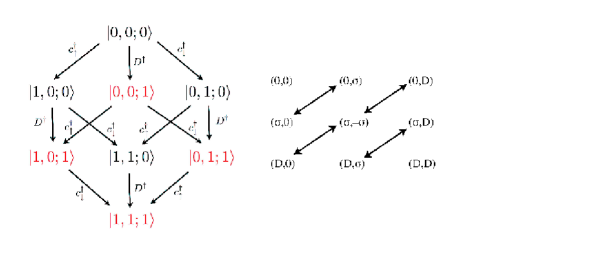
Figure 1: (a) extended Hilbert space for a single site. (b) hopping processes between neighbouring sites included in the Lagrangian. Double occupation has been replaced by $D$-occupation.

There are of course several unphysical states in this Hilbert space. As we will see, such states are removed once the constraint is solved. At present, the expansion of the Hilbert space should be thought of as a tool to enable the integration of the high energy degrees of freedom. To proceed, we formulate a Lagrangian in the extended Hilbert space. The allowed hops involving the $D$ fields and the electron operators which are equivalent to the hops in the Hubbard model are indicated in Fig(1b). For example, the hopping process in the upper left-hand corner describes the hopping of a hole in the lower-Hubbard band. The terms in the middle describe the transport between the $D$ field and two electrons in a singlet on neighbouring sites. The term in the lower right corner describes a hop in which $D_{i}$ and $c_{j}^{\dagger}$ switch places. There are no further allowable hopping processes. A further requirement of the Lagrangian for the hole-doped theory is that it contain the appropriate dynamical term for motion in the lower Hubbard band. That is, those sites which contain the occupancy $c^{\dagger}_{i,\downarrow}c^{\dagger}_{i,\uparrow}|0\rangle$ must be excluded from hopping processes (such hops are accounted for by the hopping of $D$). The Euclidean Lagrangian in the extended Hilbert space which describes the hopping processes detailed above can be written

$$L =\int d^{2}\theta\left[\bar{\theta}\theta\sum_{i,\sigma}(1-n_{i,-\sigma})c^{\dagger}_{i,\sigma}\dot{c}_{i,\sigma}+\sum_{i}D_{i}^{\dagger}\dot{D}_{i}\right.$$ (7)

$$+U\sum_{j}D^{\dagger}_{j}D_{j}-t\sum_{i,j,\sigma}g_{ij}\left[C_{ij,\sigma}c^{\dagger}_{i,\sigma}c_{j,\sigma}+D_{i}^{\dagger}c^{\dagger}_{j,\sigma}c_{i,\sigma}D_{j}\right.$$

$$+\left.\left.(D_{j}^{\dagger}\theta c_{i,\sigma}V_{\sigma}c_{j,-\sigma}+h.c.)\right]+H_{\rm con}\right].$$

Here, $g_{ij}$ selects out nearest neighbours (note that if we wanted to include next-to-nearest neighbour interactions, we need just modify the matrix $g_{ij}$ accordingly), the parameter $V_{\sigma}$ has values $V_{\uparrow}=1$, $V_{\downarrow}=-1$, and simply ensures that $D$ couples to the spin singlet and the operator $C_{ij,\sigma}$ is of the form $C_{ij,\sigma}\equiv\bar{\theta}\theta\alpha_{ij,\sigma}\equiv\bar{\theta}\theta(1-n_{i,-\sigma})(1-n_{j,-\sigma})$ with number operators $n_{i,\sigma}\equiv c^{\dagger}_{i,\sigma}c_{i,\sigma}$.

For simplicity, we have introduced a complex Grassman constant $\theta$, which we have inserted in order to keep track of statistics; it bears some resemblance to a superspace coordinate. Because $D_{j}$ is fermionic and $c_{j,\uparrow}c_{j,\downarrow}$ transforms as a boson, a Grassman variable is needed to essentially ‘fermionize’ double occupancy. They are normalized via

$$\int d^{2}\theta\ \bar{\theta}\theta=1.$$ (8)

The Grassmann variable is an artificial device that will disappear from the UV or IR Lagrangians.

The constraint Hamiltonian $H_{\rm con}$ is taken to be

$$H_{\rm con}=s\bar{\theta}\sum_{j}\varphi_{j}^{\dagger}(D_{j}-\theta c_{j,\uparrow}c_{j,\downarrow})+h.c.$$ (9)

where $\varphi$ is a complex charge $2e$ bosonic field which enters the theory as a Lagrange multiplier. The constant $s$ has been inserted to carry the units of energy. At this point, there is some ambiguity in the normalization of $\varphi$, but we expect that this will be set dynamically. We will find that if a true infrared limit exists, then $s$ must be of order the hopping matrix element $t$. There is a natural parallel between the constraint condition, Eq. (9), and the constraint in the non-linear sigma model. In fact, the auxiliary field $\varphi$ will enter the low-energy theory in an analogous fashion to $\sigma$ in the non-linear sigma model. In both cases, $\varphi$ and $\sigma$ enter as Lagrange multipliers. Both end up playing a crucial role in the phase structure of the true low-energy or infrared limit. In this case, $\varphi$ will serve to create new excitations at low energy which will generate the dynamical part of the spectral weight transfer across the Mott gap.

Now, as remarked previously, we have chosen the Lagrangian (7) so that this theory is equivalent to the Hubbard model. To demonstrate this, we first show that once the constraint is solved, we obtain the Hubbard model. Hence, the Lagrangian we have formulated is the Hubbard model written in a non-traditional form – in some sense, we have inserted unity into the Hubbard model path integral in a rather complicated fashion. To this end, we compute the partition function

$$Z=\int[{\cal D}c\ {\cal D}c^{\dagger}\ {\cal D}D\ {\cal D}D^{\dagger}\ {\cal D}\varphi\ {\cal D}\varphi^{\dagger}]\exp^{-\int_{0}^{\tau}Ldt}.$$ (10)

with $L$ given by (7). We note that $\varphi$ is a Lagrange multiplier. As shown in the Appendix (Eq. (43)), in the Euclidean signature, the fluctuations of the real and imaginary parts of $\varphi_{i}$ must be integrated along the imaginary axis for $\varphi_{i}$ to be regarded as a Lagrangian multiplier. The $\varphi$ integrations (over the real and imaginary parts) are precisely a representation of (a series of) $\delta$-functions of the form,

$$\delta\left(\int d\theta D_{i}-\int d\theta\ \theta c_{i,\uparrow}c_{i,\downarrow}\right).$$ (11)

If we wish to recover the Hubbard model, we need only to integrate over $D_{i}$, which is straightforward because of the $\delta$-functions. The dynamical terms yield

$$\int d^{2}\theta\ \bar{\theta}\theta\left[\sum_{i,\sigma}(1-n_{i,-\sigma})c^{\dagger}_{i,\sigma}\dot{c}_{i,\sigma}+\sum_{i}c^{\dagger}_{i,\downarrow}c_{i,\uparrow}^{\dagger}\dot{c}_{i,\uparrow}c_{i,\downarrow}\right.$$

$$\qquad\qquad\left.+\sum_{i}c^{\dagger}_{i,\downarrow}c_{i,\uparrow}^{\dagger}c_{i,\uparrow}\dot{c}_{i,\downarrow}\right]$$

$$=\int d^{2}\theta\ \bar{\theta}\theta\sum_{i,\sigma}\left[(1-n_{i,-\sigma})c^{\dagger}_{i,\sigma}\dot{c}_{i,\sigma}+n_{i,-\sigma}c_{i,\sigma}^{\dagger}\dot{c}_{i,\sigma}\right]$$

$$=\int d^{2}\theta\ \bar{\theta}\theta\sum_{i,\sigma}c_{i,\sigma}^{\dagger}\dot{c}_{i,\sigma}.$$ (12)

Likewise the term proportional to $V_{\sigma}$ yields

$$\int d^{2}\theta\ \bar{\theta}\theta\sum_{i,j}g_{ij}\left[c_{j,\downarrow}^{\dagger}c_{j,\uparrow}^{\dagger}(c_{i,\uparrow}c_{j,\downarrow}-c_{i,\downarrow}c_{j,\uparrow})\right]+h.c.$$

$$=\int d^{2}\theta\ \bar{\theta}\theta\sum_{i,j,\sigma}g_{ij}n_{j,-\sigma}c^{\dagger}_{j,\sigma}c_{i,\sigma}+h.c.$$ (13)

Finally, the hopping terms that involve two $D$ fields give rise to

$$\int d^{2}\theta\ \bar{\theta}\theta\sum_{i,j}g_{ij}\left[c_{i,\downarrow}^{\dagger}c_{i,\uparrow}^{\dagger}(c_{j,\uparrow}^{\dagger}c_{i,\uparrow}+c_{j,\downarrow}^{\dagger}c_{i,\downarrow})c_{j,\uparrow}c_{j,\downarrow}\right]$$

$$=-\int d^{2}\theta\ \bar{\theta}\theta\sum_{i,j}g_{ij}n_{j,-\sigma}n_{i,-\sigma}c_{i,\sigma}^{\dagger}c_{j,\sigma}.$$ (14)

Eqs. (II.1) and (II.1) add to the constrained hopping term in the Lagrangian (the term proportional to $C_{ij,\sigma}$) to yield the standard kinetic energy term in the Hubbard model. Finally, the $D^{\dagger}D$ term generates the on-site repulsion of the Hubbard model. Consequently, by integrating over $\varphi_{i}$ followed by an integration over $D_{i}$, we recover the Lagrangian,

$$\int d^{2}\theta\ \bar{\theta}\theta L_{\rm Hubb}=\sum_{i,\sigma}c_{i,\sigma}^{\dagger}\dot{c}_{i,\sigma}+H_{\rm Hubb},$$ (15)

of the Hubbard model. This constitutes the ultra-violet (UV) limit of our theory. In this limit, it is clear that the Grassman variables amount to an insertion of unity and hence play no role. Further, in this limit the extended Hilbert space contracts, unphysical states such as $|1,0,1\rangle$, $|0,1,1\rangle$, $|1,1,1\rangle$ are set to zero, and we identify $|1,1,0\rangle$ with $|0,0,1\rangle$. Note there is no contradiction between treating $D$ as fermionic and the constraint in Eq. (9). The constraint never governs the commutation relation for $D$. The value of $D$ is determined by Eq. (9) only when $\varphi$ is integrated over. This is followed immediately by an integration over $D$ at which point $D$ is eliminated from the theory.

The advantage of our starting Lagrangian over the traditional writing of the Hubbard model is that we are able to coarse grain the system cleanly for $U\gg t$. The energy scale associated with $D$ is the large on-site energy $U$. Hence, it makes sense, instead of solving the constraint, to integrate out $D$. The resultant theory will contain explicitly the bosonic field, $\varphi$. As a result of this field, double occupancy will remain, though the energy cost will be shifted from the UV to the infrared (IR). Because the theory is Gaussian, the integration over $D_{i}$ can be done exactly. This is the ultimate utility of the expansion of the Hilbert space – we have isolated the high energy physics into this Gaussian field. As a result of the dynamical term in the action, integration over $D$ will yield a theory that is frequency dependent. The frequency will enter in the combination $\omega+U$ which will appear in denominators. Since $U$ is the largest energy scale, we expand in powers of $\omega/U$; the leading term yields the proper $\omega=0$ low-energy theory. Since the theory is Gaussian, it suffices to complete the square in the $D$-field. To accomplish this, we define the matrix

$${\cal M}_{ij}=\delta_{ij}-\frac{t}{(\omega+U)}g_{ij}\sum_{\sigma}c_{j,\sigma}^{\dagger}c_{i,\sigma}$$ (16)

and $b_{i}=\sum_{j}b_{ij}=\sum_{j,\sigma}g_{ij}c_{j,\sigma}V_{\sigma}c_{i,-\sigma}$. At zero frequency the Hamiltonian is

$$H^{IR}_{h}=-t\sum_{i,j,\sigma}g_{ij}\alpha_{ij,\sigma}c^{\dagger}_{i,\sigma}c_{j,\sigma}+H_{\rm int}-\frac{1}{\beta}Tr\ln{\cal M},$$

where

$$H_{\rm int}=-\frac{t^{2}}{U}\sum_{j,k}b^{\dagger}_{j}({\cal M}^{-1})_{jk}b_{k}-\frac{s^{2}}{U}\sum_{i,j}\varphi_{i}^{\dagger}({\cal M}^{-1})_{ij}\varphi_{j}$$

$$-s\sum_{j}\varphi_{j}^{\dagger}c_{j,\uparrow}c_{j,\downarrow}+\frac{st}{U}\sum_{i,j}\varphi^{\dagger}_{i}({\cal M}^{-1})_{ij}b_{j}+h.c.$$ (17)

which constitutes the true (IR) limit as long as the energy scale $s$ is not of order $U$. If $s\sim O(U)$ then we should also integrate out $\varphi_{i}$ – this integration is again Gaussian and can be done exactly; one can easily check that this leads precisely back to the UV theory, the Hubbard model. Hence, the only way in which a low-energy theory of the Hubbard model exists is if the energy scale for the dynamics that $\varphi$ mediates is $O(t)$. This observation is significant because it lays plain the principal condition for the existence of an IR limit of the Hubbard model.

To fix $s$, we note that the fourth term entering our Hamiltonian can mediate spin exchange. As the energy scale for this process is $t^{2}/U$, we make the identification $s\simeq t$. Hence, the low-energy theory contains a charge $2e$ bosonic field which can either annihilate/create doubly occupied sites or nearest-neighbour singlets. That the energy cost for double occupancy in the IR is $t^{2}/U$ and not $U$ underscores the fact that the UHB and LHB are not orthogonal. The presence of the new field $\varphi_{i}$ at low energies is the result of the overlap between the high and low energy scales. Physically, double occupancy occurs at low energies for two distinct reasons. The first is spin exchange which is generated by the term $\varphi_{i}b_{i}^{\dagger}$. The second is motion of a doubly occupied site (a doublon) entirely in the LHB. The latter is not present in projective models but is certainly a low-energy process that must be present in the exact low-energy theory.

While electron number conservation is broken in the IR, we find (by inspection of (II.1)) that a conserved low-energy charge does existcharge

$$Q=\sum_{i,\sigma}c_{i,\sigma}^{\dagger}c_{i,\sigma}+2\sum_{i}\varphi^{\dagger}_{i}\varphi_{i}.$$ (18)

As Eq. (II.1) makes clear, bosons acquire dynamics only through electron motion. Hence, the low-energy theory of a hole-doped Mott insulator is a strongly coupled bose-fermi model. On purely phenomenological grounds, bose-fermi models have been advancedtdlee ; ranninger as a starting point for tackling the cuprate problem. In such models, and othersPert3 , the bosons are viewed as non-interacting and possess a Fock space of their own. However, the current analysis lays plain that while the bosonic degree of freedom exists, it does not extend the Hilbert space of the Hubbard model. That is, the charge $2e$ boson does not have a Fock space of its own. In obtaining the low-energy theory, we integrated over the high energy $D-$ field which acted in the extended Hilbert space. Consequently, the resultant low-energy theory preserves the original Hilbert space of the Hubbard model. As we will show, a distinct possibility is that the boson acts to create composite excitations that have charge $e$.

Several limits are of interest. First, consider the limit $U=\infty$ (for fixed lattice size). The theory reduces to the restricted hopping term and the third term in Eq. (II.1). In this limit, the $\varphi$ integration reduces to a delta function, $\delta(c_{i,\uparrow}c_{i,\downarrow})$, giving a constraint enforcing the vanishing of double occupancy, the correct result for $U=\infty$.

Second, should $\varphi=0$, we recover the interactions in the $t-J$ model. To establish this, we note that for $\varphi_{i}=0$, we have the restricted hopping term and the first term in Eq. (II.1). Approximating ${\cal M}_{ij}$ by its leading term, $\delta_{ij}$, the second term reduces to

$$\sum_{i}b_{i}^{\dagger}b_{i}=\sum_{ij\ell\sigma\sigma^{\prime}}g_{ij}g_{\ell i}c^{\dagger}_{i,-\sigma}V_{\sigma}c^{\dagger}_{j,\sigma}c_{\ell,\sigma^{\prime}}V_{\sigma^{\prime}}c_{i,-\sigma^{\prime}}$$ (19)

which contains the spin-spin interaction $-({\mathbf{S}}_{i}\cdot{\mathbf{S}}_{j}-n_{i}n_{j}/4)$ as well as the three-site hopping term. Next, we expand the $Tr\ln$ term

$$Tr\ln{\cal M}^{-1} = Tr\ln(\delta_{ij}+A_{ij})$$

$$= A_{ii}+\frac{1}{2}A_{ij}A_{ji}+\ldots$$

$$= \frac{t^{2}}{(\omega+U)^{2}}\sum_{\sigma,\sigma^{\prime}}\sum_{i,j}g_{ij}c_{j,\sigma}^{\dagger}c_{i,\sigma}c_{i,\sigma^{\prime}}^{\dagger}c_{j,\sigma^{\prime}}+\ldots$$

where

$$A_{ij}=\frac{t}{\omega+U}\sum_{\sigma}g_{ij}c_{j,\sigma}^{\dagger}c_{i,\sigma}$$ (20)

is nonzero only if $i,j$ are nearest neighbours. When this term appears in the Euclidean Lagrangian, its magnitude is $k_{B}Tt^{2}/(\omega+U)^{2}$. Therefore, at low temperature, this term is small compared to $H_{\rm IR}$ and to leading order in $t^{2}/U$, the terms in $H_{\rm IR}$ dominate. Hence, the $\varphi=0$ limit contains the interactions in the $t-J$ model, thereby establishing that the physics contained in $\varphi_{i}$ is non-projective. To make closer contact with the $t-J$ model in which the spin-spin interaction acts only in the singly-occupied sector, we note that the theory we have developed here could have been formulated strictly in the projected space by simply substituting $\xi_{i,\sigma}$ for $c_{i,\sigma}$ in the hopping terms containing $D_{i}$ in our starting Lagrangian, Eq. (7). The only substantive difference would be that the second hopping term (the term quadratic in $D_{i}$) in Eq. (7) would enter with the opposite sign. Hence, in the IR limit, ${\cal M}_{ij}\rightarrow\delta_{ij}+t/U\xi_{j,\sigma}^{\dagger}\xi_{i,\sigma}$. This change is dictated by the commutation relations of the $\xi_{i,\sigma}$ operators. The UV limit, the Hubbard model, is obtained as before. Setting $\varphi_{i}=0$ in the IR limit leads exactly to the $t-J$ model. Thus, the $t-J$ modelPert33 written in terms of the bare electron operators is not the low-energy limit of the Hubbard model. This is not entirely surprising as Eskes and otherseskes has stressed that the operators must be transformed as well in writing the $t-J$ model. Only at $U=\infty$ do the transformed and bare fermion operators agree. Hence, at any finite $U$, the physics is governed by a finite length scale for double occupancy. Hence the limits $U\rightarrow\infty$ and $L\rightarrow\infty$ (L the size of the system) do not commute as is required for a hard projective model (no double occupancy in the original electron basis) to be the true low-energy theory of the Hubbard model.

No such problem besets our low-energy theory. We can recover the original Hubbard model from our low-energy theory by simply integrating over $\varphi_{i}$. Although this is not a sensible thing to do from a low energy perspective, it can be done exactly. To see how this happens, we rewrite Eq. (II.1) including the frequency dependence,

$$L_{IR} = \sum_{i,\sigma}(1-n_{i\bar{\sigma}})c_{i,\sigma}^{\dagger}\dot{c}_{i,\sigma}-t\sum_{i,\sigma}(1-n_{i\bar{\sigma}})c_{i,\sigma}^{\dagger}c_{j,\sigma}(1-n_{j\bar{\sigma}})$$

$$- \sum_{ij}\left(s\varphi_{i}^{\dagger}-t\sum_{\langle i,k\rangle}b_{ki}^{\dagger}+(\omega+\hat{U})c^{\dagger}_{k\downarrow}c^{\dagger}_{k\uparrow}{\cal M}_{ki}\right)$$

$$\times\frac{({\cal M}^{-1})_{ij}}{\omega+\hat{U}}\left(s\varphi_{j}-t\sum_{\langle j,n\rangle}b_{nj}+(\omega+\hat{U}){\cal M}_{jn}c_{n\uparrow}c_{n\downarrow}\right)$$

$$- tc_{i,\downarrow}^{\dagger}c_{i,\uparrow}^{\dagger}b_{i}-tb_{i}^{\dagger}c_{i,\uparrow}c_{i,\downarrow}+(\omega+\hat{U})c_{i,\downarrow}^{\dagger}c_{i,\uparrow}^{\dagger}{\cal M}_{ij}c_{j,\uparrow}c_{j,\downarrow}$$

$$- \frac{1}{\beta}Tr\ln{\cal M}$$

To simplify the expression, note that,

$$-tb_{i}^{\dagger}c_{i,\uparrow}c_{i,\downarrow} = -t\sum_{j}(c_{i,\downarrow}^{\dagger}c_{j,\uparrow}^{\dagger}-c_{i,\uparrow}^{\dagger}c_{j,\downarrow}^{\dagger})c_{i,\uparrow}c_{i,\downarrow}$$ (21)

$$= -t\sum_{\sigma}c_{j,\sigma}^{\dagger}c_{i,\sigma}n_{i,-\sigma}$$

and

$$-\sum_{\langle i,j\rangle\sigma}c_{i,\downarrow}^{\dagger}c_{i,\uparrow}^{\dagger}c_{j,\sigma}^{\dagger}c_{i,\sigma}c_{j,\uparrow}c_{j,\downarrow}=\sum_{\langle i,j\rangle,\sigma}n_{i,-\sigma}c_{i,\sigma}^{\dagger}c_{j,\sigma}n_{j,-\sigma}.$$ (22)

which comes from $c_{i,\downarrow}^{\dagger}c_{i,\uparrow}^{\dagger}{\cal M}_{ij}c_{j,\uparrow}c_{j,\downarrow}$. The Lagrangian becomes

$$L = \sum_{i,\sigma}c_{i,\sigma}^{\dagger}\dot{c}_{i,\sigma}+H_{Hubb}$$ (23)

$$- \sum_{ij}\left(s\varphi_{i}^{\dagger}-t\sum_{\langle i,k\rangle}b_{ki}^{\dagger}+(\omega+\hat{U})c^{\dagger}_{k\downarrow}c^{\dagger}_{k\uparrow}{\cal M}_{ki}\right)$$

$$\frac{({\cal M}^{-1})_{ij}}{\omega+U}\left(s\varphi_{j}-t\sum_{\langle j,n\rangle}b_{nj}+(\omega+\hat{U}){\cal M}_{jn}c_{n\uparrow}c_{n\downarrow}\right)$$

$$-\frac{1}{\beta}Tr\ln{\cal M}$$

which yields the Hubbard model upon integration over $\varphi_{i}$ (see the Appendix for details).

We conclude from this analysis that our low-energy theory permits immediate correspondence with the original Hubbard model; that is, we have not lost any information regarding the high energy scale, unlike projective methods. All information regarding the high-energy scale is encoded into the emergent charge $2e$ bosonic excitation and its interactions. The IR physics will be determined by examining the low energy dynamics of the electrons/holes and $\varphi$.

II.2 What this theory is not

Rather than decoupling the on-site repulsion term, we derived our low-energy theory by exponentiating a $\delta-$functional constraint on the heavy field, $D$. Nonetheless, one might contemplate that our theory could be obtained by more traditional schemes, for example by some sort of Hubbard Stratonovich (HS) decoupling scheme. Since the interaction in the Hubbard model is entirely local, any decoupling by means of introducing an auxiliary field would yield only local interactions. The auxiliary field $\varphi_{i}$ in Eq. (II.1) clearly generates non-local interactions as well as on-site interactions. Hence, Eq. (II.1) cannot be obtained from a HS transformation. However, the non-local terms are scaled by $t/U$. Hence, it might still be maintained that the local terms dominate and in fact that they could be obtained by some sort of HS transformation. Consider the identity,

$$e^{-UX^{\dagger}X}=\int d^{2}\sigma\ e^{-(\lambda\sigma^{\dagger}\sigma+\lambda_{1}\sigma X^{\dagger}+\lambda_{2}X\sigma^{\dagger})}$$ (24)

which is true as long as $\lambda\in\mathbb{R}^{+}$ and $\lambda_{1}\lambda_{2}=-U\lambda$. The standard HS transformation assumes that $\lambda_{1}\lambda_{2}\in\mathbb{R}^{+}$ and $\lambda_{2}=\lambda_{1}^{\ast}$. This necessarily leads only to the $-U$ Hubbard model with $X=c_{\uparrow}c_{\downarrow}$. However, the constraint that the exponent on the right-hand side of Eq. (24) be real can be relaxedcomplex in which case it can be applied to the $+U$ Hubbard model as well. Nonetheless, this procedure will not yield the non-local terms in our low-energy theory. Further, it does not permit a clean identification of the field associated with the high-energy degrees of freedom. That is, there is no D-field in any version of Eq. (24). Consequently, this procedure is a non-starter for the construction of a proper low-energy theory.

II.3 Electron doping

For electron doping, the chemical potential jumps to the bottom of the UHB. Consequently, the degrees of freedom that lie far away from the chemical potential no longer correspond to double occupancy but rather double holes. To coarse grain these degrees of freedom, we extend the Hilbert space in a similar way as the hole-doped theory, defining a new field $\tilde{D}$ which will be constrained to describe the creation of double holes. Mathematically, all results in hole doping obtained in the previous section can be transformed to electron doping via a generalized particle-hole transformation (GPHT), namely,

$$c_{i,\sigma} \rightarrow e^{i{\mathbf{Q}}\cdot{\mathbf{R}}_{i}}c_{i,\sigma}^{\dagger}$$

$$D_{i} \rightarrow \tilde{D}_{i}$$

$$\varphi_{i} \rightarrow \tilde{\varphi}_{i}$$ (25)

where ${\mathbf{Q}}=(\pi,\pi)$ and $\tilde{D}_{i}$ is a fermion operator associated with double holes. The new bosonic field, $\tilde{\varphi}$, is the Lagrangian multiplier defined by the constraint, $\tilde{H}_{\rm con}=\tilde{s}\bar{\theta}\sum_{i}\tilde{\varphi}_{i}(\tilde{D}_{i}-\theta c_{i,\uparrow}^{\dagger}c_{i,\downarrow}^{\dagger})+h.c.$. According to Eq. (7), an appropriate Lagrangian for the extended theory at electron doped can be constructed,

$$L =\int d^{2}\theta\left[\bar{\theta}\theta\sum_{i,\sigma}n_{i,-\sigma}c_{i,\sigma}\dot{c}_{i,\sigma}^{\dagger}+\sum_{i}\tilde{D}_{i}^{\dagger}\dot{\tilde{D}}_{i}+U\sum_{j}\tilde{D}_{j}^{\dagger}\tilde{D}_{j}\right.$$ (26)

$$-t\sum_{i,j,\sigma}g_{ij}\left[c^{\dagger}_{i,\sigma}n_{i,-\sigma}c_{j,\sigma}n_{j,-\sigma}+\tilde{D}_{j}^{\dagger}c^{\dagger}_{j,\sigma}c_{i,\sigma}\tilde{D}_{i}\right.$$

$$+\left.\left.(\bar{\theta}c_{i,\sigma}V_{\sigma}c_{j,-\sigma}\tilde{D}_{i}+h.c.)\right]+\tilde{H}_{\rm con}\right],$$

that preserves the distinct hops in the Hubbard model. Two differences to note are that 1) because the chemical potential resides in the UHB, the electron hopping term now involves sites that are at least singly occupied and 2) the order of the $\tilde{D}_{i}$ and $c_{i}$ operators is important. If we integrate over $\tilde{\varphi}_{i}$ and then $\tilde{D}_{i}$, all the unphysical states are removed and we obtain as before precisely $L_{\rm Hubb}$. Hence, both theories yield the Hubbard model in their UV limits. They differ, however, in the IR as can be seen by performing the integration over $\tilde{D}_{i}$. The corresponding integral is again Gaussian and yields

$$H^{IR}_{\rm e}=-t\sum_{i,j,\sigma}g_{ij}c^{\dagger}_{i,\sigma}n_{i,-\sigma}c_{j,\sigma}n_{j,-\sigma}+\tilde{H}_{\rm int}-\frac{1}{\beta}Tr\ln{\cal\tilde{M}}$$

where

$$\tilde{H}_{\rm int} = -\frac{t^{2}}{U}\sum_{j,k}b_{j}({\cal\tilde{M}}^{-1})_{jk}b^{\dagger}_{k}-\frac{\tilde{s}^{2}}{U}\sum_{i,j}\tilde{\varphi}_{i}^{\dagger}({\cal\tilde{M}}^{-1})_{ij}\tilde{\varphi}_{j}$$

$$-\tilde{s}\sum_{j}\tilde{\varphi}_{j}^{\dagger}c_{j,\uparrow}^{\dagger}c_{j,\downarrow}^{\dagger}+\frac{\tilde{s}t}{U}\sum_{i,j}\tilde{\varphi}^{\dagger}_{i}({\cal\tilde{M}}^{-1})_{ij}b_{j}^{\dagger}+h.c.$$

as the IR limit of the electron-doped theory. In Eq.(II.3), the matrix ${\cal\tilde{M}}_{ij}={\cal M}_{ji}$ is defined via the GPHT on the ${\cal M}$ matrix in Eq.(16). As $\tilde{\varphi}_{i}$ is a complex field, the GPHT interchanges the creation operators of opposite charge. We again make the identification $\tilde{s}\sim t$ because the last term can also mediate spin exchange.

When the boson vanishes, we do recover the exact particle-hole symmetric analogue of the hole-doped theory. Because the field $\tilde{\varphi}$ now couples to double holes, the relevant creation operator has charge $-2e$ and the conserved charge is $\tilde{Q}=\sum_{i,\sigma}c_{i,\sigma}^{\dagger}c_{i,\sigma}-2\varphi_{i}^{\dagger}\varphi_{i}$. This sign change in the conserved charge will manifest itself as a sign change in the chemical potential as long as $\langle\tilde{\varphi}_{i}^{\dagger}\tilde{\varphi}_{i}\rangle\neq 0$. Likewise, the correct $U\rightarrow\infty$ limit is obtained as before.

II.4 Half Filled Models

At half filling when the chemical potential lies within the Mott gap, both double hole and double occupancy lie far away from the chemical potential. As two different degree of freedom per site need to be coarse grained, we introduce two new fields $D$ and $\tilde{D}$ which when constrained correspond to double occupancy and double holes, respectively and extend the Hilbert space to $\otimes_{i}\left({\cal F}_{\uparrow}\otimes{\cal F}_{\downarrow}\otimes{\cal F}_{D}\otimes{\cal F}_{\tilde{D}}\right)$. The corresponding low-energy theory will be obtained by integrating over both $D$ and $\tilde{D}$ rather than by solving the constraint. As a result, integrating over $D$ and $\tilde{D}$ do not yield identical results as would be the case if double occupancy or double holes were integrated over.

II.4.1 Anderson Impurity

To illustrate the process of coarse graining two high energy fields, we begin with a simpler model, the Andersonaimp impurity model.

$$H = E_{f}(n_{\uparrow}+n_{\downarrow})+Un_{\downarrow}n_{\uparrow}$$ (27)

$$+ \sum_{{\mathbf{k}},\sigma}n_{{\mathbf{k}},\sigma}\varepsilon_{{\mathbf{k}}}+\sum_{{\mathbf{k}}}\left(v_{{\mathbf{k}}}c_{{\mathbf{k}},\sigma}^{\dagger}a_{\sigma}+h.c.\right)$$

where $a_{\sigma}$ destroys an impurity electron and $c_{{\mathbf{k}},\sigma}$ destroys a continuum electron. By setting $E_{f}=-U/2$, it costs an energy $U/2$ to create an double hole or a doubly occupied states on the impurity site which is analogous to the half-filled Hubbard model. In the following, we would like to show, by introducing two heavy fields $D$ and $\tilde{D}$ which correspond to the doubly occupied or double hole states on the impurity site respectively, the Kondo model with additional coupling to new bosonic fields can be derived perturbatively if $v_{{\mathbf{k}}}\ll U$.

The appropriate extended Hamiltonian is

$$H = \int d^{2}\theta\left[E_{f}\sum_{\sigma}n_{\sigma}+\frac{1}{2}UD^{\dagger}D-\frac{1}{2}U\tilde{D}\tilde{D}^{\dagger}+\bar{\theta}\theta\sum_{{\mathbf{,}}\sigma}n_{{\mathbf{k}},\sigma}\varepsilon_{{\mathbf{k}}}+\sum_{{\mathbf{k}},\sigma}\left(\bar{\theta}c_{{\mathbf{k}},-\sigma}^{\dagger}V_{\sigma}a_{\sigma}^{\dagger}D+\bar{D}^{\dagger}\theta c_{{\mathbf{k}},-\sigma}^{\dagger}V_{\sigma}a_{\sigma}^{\dagger}+h.c.\right)\right.$$ (28)

$$\left.+s\bar{\theta}\varphi^{\dagger}\left(D-\theta a_{\uparrow}a_{\downarrow}\right)+h.c.+\tilde{s}\bar{\theta}\tilde{\varphi}^{\dagger}\left(\tilde{D}-\theta a_{\uparrow}^{\dagger}a_{\downarrow}^{\dagger}\right)+h.c.\right],$$

In the current model, two bosonic field $\varphi$ and $\tilde{\varphi}$ are introduced which corresponding to the two constraints on $D$ and $\tilde{D}$ fields respectively. If we first integrate out $\varphi$, $\tilde{\varphi}$ which result in delta functions corresponding to the removal of the unphysical states and then integrate out $D$ and $\tilde{D}$, Eq. (27) is obtained precisely. This constitutes the ultra-violet (UV) limit of this theory. Similar to the previous discussions, we can derive the IR limit of the Anderson impurity model by first integrating out both $D$ and $\tilde{D}$ fields, which amounts to substituting

$$D^{\dagger} = -\frac{2}{U}\bar{\theta}\left(s\varphi^{\dagger}+\sum_{{\mathbf{k}},\sigma}v_{{\mathbf{k}}}c_{{\mathbf{k}},\sigma}^{\dagger}V_{\sigma}a^{\dagger}_{\sigma}\right)$$ (29)

$$\tilde{D} = -\frac{2}{U}\left(\tilde{s}\varphi+\sum_{{\mathbf{k}},\sigma}v_{{\mathbf{k}}}c_{{\mathbf{k}},\sigma}^{\dagger}V_{\sigma}a^{\dagger}_{\sigma}\right)\theta$$ (30)

into $H$. We finally obtain

$$H_{IR} = H_{\rm Kondo}-\frac{2}{U}(s^{2}\varphi^{\dagger}\varphi+\tilde{s}^{2}\tilde{\varphi}^{\dagger}\tilde{\varphi})-(s\varphi^{\dagger}+\tilde{s}\tilde{\varphi}^{\dagger})a_{\uparrow}a_{\downarrow}$$ (31)

$$- \frac{2}{U}(s\varphi^{\dagger}+\tilde{s}\tilde{\varphi})\sum_{{\mathbf{k}},\sigma}v_{{\mathbf{k}}}a_{\sigma}V_{\sigma}c_{{\mathbf{k}},\sigma}+h.c.$$

where $H_{\rm Kondo}$ is the Kondo Hamiltonian

$$H_{\rm Kondo} = \sum_{{\mathbf{k}},\sigma}n_{{\mathbf{k}},\sigma}\varepsilon_{{\mathbf{k}}}-\frac{U}{2}(n_{\uparrow}+n_{\downarrow})$$ (32)

$$+\sum_{{\mathbf{k}},{\mathbf{k}}^{\prime}}\frac{4v_{{\mathbf{k}}}v_{{\mathbf{k}}^{\prime}}}{U}\left[(c_{{\mathbf{k}}}^{\dagger}\overrightarrow{\sigma}c_{{\mathbf{k}}^{\prime}})\cdot{\mathbf{S}}_{imp}\right.$$

$$\left.-\frac{1}{2}c_{{\mathbf{k}}}^{\dagger}c_{{\mathbf{k}}^{\prime}}(n_{\uparrow}+n_{\downarrow})\right].$$

Here, ${\mathbf{S}}_{imp}=a^{\dagger}_{\sigma}\overrightarrow{\sigma}_{\sigma\sigma^{\prime}}a_{\sigma}^{\prime}$ is the spin operator of the impurity site. Thus the IR limit consists of the Kondo model in addition to the coupling between the electron and the new bosonic degree of freedom.

II.4.2 Half-filled Hubbard Model

Next, we perform the same procedure for the Hubbard model at half-filling by introducing two new fermionic fields $D$ and $\tilde{D}$ associated with the double occupancy and double holes, respectively. We consider the generalised Lagrangian

$$L = \int d^{2}\theta\left[\sum_{i}(D_{i}^{\dagger}\dot{D}_{i}+\dot{\tilde{D}}_{i}^{\dagger}{\tilde{D}}_{i})\right.$$ (33)

$$\left.-\frac{t}{2}\sum_{i,j,\sigma}g_{ij}\left(D_{j}^{\dagger}\theta c_{i,\sigma}V_{\sigma}c_{j,-\sigma}+\bar{\theta}c_{i,\sigma}V_{\sigma}c_{j,-\sigma}\tilde{D}_{j}+h.c.\right)\right.$$

$$\left.+\frac{U}{2}\sum_{j}(D_{j}^{\dagger}D_{j}-\tilde{D}_{j}\tilde{D}_{j}^{\dagger})+H_{con}\right]$$

with the constraint terms given by

$$H_{con} = s\bar{\theta}\sum_{i}\varphi_{i}^{\dagger}(D_{i}-\theta c_{i,\uparrow}c_{i,\downarrow})+h.c.$$ (34)

$$+ \tilde{s}\bar{\theta}\sum_{i}\tilde{\varphi}_{i}^{\dagger}(\tilde{D}_{i}-\theta c_{i,\uparrow}^{\dagger}c_{i,\downarrow}^{\dagger})+h.c.$$

Here, $\varphi_{i}$ and $\tilde{\varphi}_{i}$ are two the bosonic field with charge $2e$ and $-2e$ respectively. Similar to the previous result, if we first integrate out both the bosonic fields $\varphi_{i}$, $\tilde{\varphi}_{i}$ and then $D_{i}$, $\tilde{D}_{i}$, the Hubbard model is obtained and the generalised theory Eq. 33 yields the correct UV limit. However, a different IR limit is obtained if we first integrate out $D_{i}$ and $\tilde{D}_{i}$,

$$H^{\rm hf}_{\rm IR} = -\frac{t^{2}}{2U}\sum_{i}\left(b_{i}^{\dagger}b_{i}+b_{i}b_{i}^{\dagger}\right)-\sum_{i}(\frac{2s^{2}}{U}\varphi_{i}^{\dagger}\varphi_{i}+\frac{2\tilde{s}^{2}}{U}\tilde{\varphi}_{i}^{\dagger}\tilde{\varphi}_{i})$$ (35)

$$+\frac{t}{U}\sum_{i}(s\varphi_{i}^{\dagger}+\tilde{s}\tilde{\varphi}_{i})b_{i}+h.c.$$

$$-\sum_{i}\ (s\varphi_{i}^{\dagger}-\tilde{s}\tilde{\varphi}_{i})c_{i,\uparrow}c_{i,\downarrow}+h.c.$$

This Hamiltonian is invariant under the transformation $c_{i,\sigma}\rightarrow\exp(i{\mathbf{Q}}\cdot{\mathbf{R}}_{i})c_{i,\sigma}^{\dagger}$, $\varphi_{i}\leftrightarrow\tilde{\varphi}_{i}$ and $s\leftrightarrow\tilde{s}$. This invariant reflects the symmetry between the double occupancy and the double hole in the system at half filling. In contrast to the doped case as in Eqs. (II.1) and (II.3), no $\cal M$ matrices appear in the IR theory at half filling. Consequently, we arrive at a closed form for the low-energy theory at half-filling. The $b^{\dagger}b+bb^{\dagger}$ terms include a spin-spin interaction as well as a three-site hopping term. However, at half-filling, the three-site hopping term vanishes. As a result,charge dynamics appear solely from motion of the charge $2e$ boson. This state of affairs obtains because at half-filling, charge dynamics persists only on the energy scale $U$. Since it is the boson that encodes the high-energy scale, it stands to reason that only the boson term mediates charge transport. As we show in Appendix A, it is the $\varphi_{i}$ terms that break the spurious local SU(2) symmetrylsu2 of the Heisenberg model and reinstate the global SU(2) symmetry of the Hubbard model. The local SU(2) symmetry in the Heisenberg model arose entirely from projection. This local SU(2) symmetry was noticed quite some time earlierlsu2 but its origin was never clarified. In fact, it is straightforward to check that in the lower-Hubbard band at half-filling, all perturbative terms in $t/U$ only mediate spin physics and hence preserve the local SU(2) symmetry of the Heisenberg model. Our derivation (see Appendix B) lays plain that as a result of the boson terms, this symmetry is absent from the true low-energy theory of the Hubbard model. Note, in the Anderson impurity models, the bosonic terms play a similar role to destroy the local SU(2) symmetry that appears as a result of projection.

Second, the true low-energy model preserves the sum rules associated with the original model. An essential propertydzy ; zeros of the half-filled Hubbard model when $U\gg t$ is the presence of a surface in momentum space (the Luttinger surface) where the single-particle Green function vanishes. Since the Mott state at half-filling has a gap, the non-trivial implication of the zero surface is that the real part of the Green function,

$$R_{\sigma}({\mathbf{k}},0)=-\int_{-\infty}^{-\Delta_{-}}d\epsilon^{\prime}\frac{A_{\sigma}({\mathbf{k}},\epsilon^{\prime})}{\epsilon^{\prime}}-\int_{\Delta_{+}}^{\infty}d\epsilon^{\prime}\frac{A_{\sigma}({\mathbf{k}},\epsilon^{\prime})}{\epsilon^{\prime}}$$ (36)

vanishes. Here $A_{\sigma}(k,\epsilon)$ is the single-particle spectral function which we are assuming to have a gap of width $2\Delta$ symmetrically located about the chemical potential at $\epsilon=0$. Because $A({\mathbf{k}},\epsilon)>0$ away from the gap, and $\epsilon$ changes sign above and below the gap, Eq. (36) can pass through zero. For this state of affairs to obtain, the piecesof the integral below and above the gap must be retained. Projected models which throw away the UHB fail to recover the zero surface. What Eq. (35) makes clear is that all the information regarding the surface of zeros is now encoded into the bosonic fields $\varphi_{i}$ and $\bar{\varphi}_{i}$. On the Luttinger surface, the self-energy diverges, representing a break-down of perturbation theory. As the bosonic fields cannot be obtained from perturbation theory, we conclude that it is the emergence of the bosonic field that accounts for the breakdown of Luttinger’s theoremzeros and ultimately the Mott insulating state.

II.5 Electron Operator

In each of the low energy theories, the operator which creates a single electron represents a composite excitation. To determine its form, we add to each of the starting Lagrangians a source term that generates the canonical electron operator when the constraint is solved. The appropriate transformation that yields the canonical electron operator in the UV, is

$$L\rightarrow L+\sum_{i,\sigma}J_{i,\sigma}\left[\bar{\theta}\theta(1-n_{i,-\sigma})c_{i,\sigma}^{\dagger}-V_{\sigma}D_{i}^{\dagger}\theta c_{i,-\sigma}\right]+h.c.$$

However, in the IR in which we only integrate over the heavy degree of freedom, $D_{i}$, the electron creation operator

$$c^{\dagger}_{i,\sigma} \rightarrow (1-n_{i,-\sigma})c_{i,\sigma}^{\dagger}-V_{\sigma}\frac{t}{U}b_{j}^{\dagger}{\cal M}_{ji}^{-1}c_{i,-\sigma}$$ (37)

$$+ V_{\sigma}\frac{s}{U}\varphi_{j}^{\dagger}{\cal M}_{ji}^{-1}c_{i,-\sigma}.$$

For electron doping, we apply the generalized particle-hole transformation to obtain

$$c^{\dagger}_{i,\sigma} \rightarrow n_{i,-\sigma}c_{i,\sigma}^{\dagger}-V_{\sigma}\frac{t}{U}c_{i,-\sigma}{\cal M}_{ij}^{-1}b_{j}^{\dagger}$$ (38)

$$+ V_{\sigma}\frac{s}{U}c_{i,-\sigma}{\cal M}_{ij}^{-1}\tilde{\varphi}_{j}.$$

as the generator of electron excitations in the IR. For either doping, the electron operator contains the standard term for motion in the LHB, $(1-n_{i,-\sigma})c_{i,\sigma}^{\dagger}$ ($n_{i,-\sigma}c_{i,\sigma})$ in the UHB for electron doping) with a renormalization from spin fluctuations (second term) and a new charge $e$ excitation, $\varphi_{j}^{\dagger}{\cal M}_{ji}^{-1}c_{i,-\sigma}$. Consequently, we predict that an electron at low energies is in a superposition of the standard LHB state (modified with spin fluctuations) and a new composite charge $e$ state described by $c_{i,-\sigma}{\cal M}_{ij}^{-1}\varphi_{j}^{\dagger}$. It is the presence of these two distinct excitations that preserves the dynamical (hopping dependent) part of the spectral weight transfer across the Mott gap. As shown in companion paperftmexp , there are also experimental ramifications for the composite structure of the electron.

At half-filling, a similar trick can be applied to generate the electron operator. In this case,

$$L\rightarrow L+\sum_{i,\sigma}J_{i,\sigma}\left[V_{\sigma}D_{i}^{\dagger}c_{i,-\sigma}\theta+V_{\sigma}\bar{\theta}c_{i,-\sigma}\tilde{D}_{i}\right]+h.c.$$

is the correct transformation to generate the canonical electron operator in the UV. If we now integrate the partition function over $D_{i}$ and $\tilde{D}_{i}$, we find that the electron creation operator at half-filling

$$c_{i,\sigma}^{\dagger}\rightarrow-V_{\sigma}\frac{t}{U}\left(c_{i,-\sigma}b_{i}^{\dagger}+b_{i}^{\dagger}c_{i,-\sigma}\right)+V_{\sigma}\frac{2}{U}\left(s\varphi_{i}^{\dagger}+\tilde{s}\tilde{\varphi}_{i}\right)c_{i,-\sigma}$$

has two important differences with its counterpart for $n\neq 1$. First, it lacks the standard LHB and UHB components as the chemical potential lies between both bands at half-filling. Second, the propagator ${\cal M}$ is absent. Nonetheless, the electron at half-filling still has two components both above and below the chemical potential. The simplification that $c_{i,-\sigma}\varphi_{i}^{\dagger}$ (that is, the ${\cal M}$ matrix is absent) constitutes the new charge $e$ excitation may make subsequent calculations of the strength of the binding between the boson and a hole at least tractable within the framework of the Bethe-Saltpeter equations.

III Final Remarks

We have shown that a true low-energy theory of a doped Mott insulator possesses degrees of freedom which do not have the quantum numbers of the electron. The degree of freedom is a local non-retarded charge $2e$ boson and hence stands in stark contrast to the charge $e$ boson in the slave bosonSlave1 ; Slave2 ; Slave3 approach in which a direct integration of the high energy scale is not possible. Fundamental to theory here is that the boson does not act in its own Fock space, in contrast to other Fermi-Bose modelstdlee ; ranninger . That is, there are no free charge 2e boson states just as there are no free quark states in confining theories. Rather, the charge 2e boson mediates new electronic states by forming composite excitations. As such the charge 2e degree of freedom is detectableletter ; ftmexp through the substructure it provides in the electron excitation spectrum. In addition, the boson is not minimally coupled to the electromagnetic gauge field. It acquires dynamics and hence a gauge coupling through high order terms in the ${\cal M}$ matrix, essentially $t^{3}/U^{2}$. At half-filling, the bosonic mode preserves the Luttinger surface on which the self-energy diverges or equivalently, the single-particle Green function vanishes. Since the boson represents a non-perturbative effect, it is not surprising that the Luttinger surface cannot occur without it. In a future publicationftmexp we explore the role of the boson in mediating the normal state properties of the cuprates as well as the possibility that the Mott state is ultimately characterized by charge neutral bound states mediated by the hidden charge $\pm 2e$ boson.

IV Appendix A: Lagrange Multipliers

Here we offer some details about the mechanics of Lagrange multipliers. Though this is standard stuff, we review it to avoid any confusion in our derivation. To illustrate the method, we will begin with the familiar example of the non-linear $\sigma$-model, that is a bosonic theory with spherical target manifold. In Lorentzian signature, we introduce the spherical constraint by writing the corresponding functional $\delta$-function as an integral of a complex exponential, with Lagrange multiplier $\sigma$:

$$Z_{L}[J] = \int[d\phi^{a}d\sigma]\ e^{i\int d^{d}x\ \left\{\frac{1}{2}\phi^{a}\partial^{2}\phi^{a}\right\}}e^{-\frac{i}{2}\int d^{d}x\ \sigma\left(\phi^{a}\phi^{a}-N/g\right)}$$ (39)

which after Wick rotation becomes

$$Z_{E}[J] = \int[d\phi^{a}d\sigma]\ e^{-\int d^{d}x\ \left\{\frac{1}{2}\phi^{a}(-\partial^{2}+\sigma)\phi^{a}-\frac{N}{2g}\sigma\right\}}$$ (40)

$$= \int[d\sigma]\ e^{-NS_{eff}(\sigma)}$$ (41)

with

$$S_{eff}(\sigma)=\frac{1}{2}Tr\ln(-\partial^{2}+\sigma)-\frac{1}{2g}\int_{x}\ \sigma$$ (42)

In eq. (41), we have performed the $\phi^{a}$ functional integrations. To proceed with the analysis of the model, we investigate (42) by expanding $\sigma$ around its vev $\langle\sigma\rangle$. It is crucial though to appreciate that if we go back to eq. (40), we see that in order for $\sigma$ to be a Lagrange multiplier field (in the Euclidean formulation), the fluctuations in $\sigma$ should be taken along the imaginary axis in field space. That is, we write

$$\sigma(x)=\langle\sigma\rangle+\frac{i}{\sqrt{N}}\lambda(x).$$ (43)

For uniform $\langle\sigma\rangle$, we then obtain

$$Tr\ln(-\partial^{2}+\sigma)=-Tr\ln\Delta_{0}+\frac{i}{\sqrt{N}}\Delta_{0}(0)\int_{x}\lambda(x)+\frac{1}{2N}\int_{x,y}\Delta_{0}(x,y)\lambda(y)\Delta_{0}(y,x)\lambda(x)+\ldots$$ (44)

where $\Delta_{0}^{-1}=-\partial^{2}+\langle\sigma\rangle$. We thus find

$$S_{eff}=-\frac{\langle\sigma\rangle}{2g}V_{d}-\frac{1}{2}Tr\ln\Delta_{0}-\frac{i}{2g\sqrt{N}}\int_{x}\lambda(x)\left(1-g\Delta_{0}(0)\right)+\frac{1}{4N}\int_{x,y}\Delta_{0}(x,y)\lambda(y)\Delta_{0}(y,x)\lambda(x)+\ldots$$ (45)

Thus we see that there is a stable saddle point giving the familiar gap equation

$$\frac{1}{g}=\int\frac{d^{d}p}{(2\pi)^{d}}\ \frac{1}{p^{2}+\langle\sigma\rangle}$$ (46)

Now, in the theory considered in this paper, we have a similar situation. In the Lorentzian signature, we have

$$Z=\int[{\cal D}c\ {\cal D}c^{\dagger}\ {\cal D}D\ {\cal D}D^{\dagger}\ {\cal D}\varphi\ {\cal D}\varphi^{\dagger}]\exp^{i\int d^{d}x(L_{0}+H_{\rm con})},$$

where

$$L_{0} = \int d^{2}\theta\left[\bar{\theta}\theta\sum_{i,\sigma}(1-n_{i,-\sigma})c^{\dagger}_{i,\sigma}\dot{c}_{i,\sigma}+\sum_{i}D_{i}^{\dagger}\dot{D}_{i}\right.$$ (48)

$$+U\sum_{j}D^{\dagger}_{j}D_{j}-t\sum_{i,j,\sigma}g_{ij}\left[C_{ij,\sigma}c^{\dagger}_{i,\sigma}c_{j,\sigma}+D_{i}^{\dagger}c^{\dagger}_{j,\sigma}c_{i,\sigma}D_{j}\right.$$

$$+\left.\left.(D_{j}^{\dagger}\theta c_{i,\sigma}V_{\sigma}c_{j,-\sigma}+h.c.)\right]\right].$$

Here again, we have written the functional $\delta-$function constraint as the integral of a complex exponential. In this case, however, $\varphi_{i}$ the Lagrange multiplier is a complex field such that $\varphi_{i}^{\ast}=\Re\varphi_{i}-i\Im\varphi_{i}$. After Wick rotation, we obtain the path integral in Euclidean signature,

$$Z=\int[{\cal D}c\ {\cal D}c^{\dagger}\ {\cal D}D\ {\cal D}D^{\dagger}\ {\cal D}\varphi\ {\cal D}\varphi^{\dagger}]\exp^{-\int d^{d}x(L_{0}+H_{\rm con})}.$$

In either the Lorentz or Euclidean signatures, $\varphi_{i}$ is a Lagrange multiplier. That is, the integral over $\varphi_{i}$ must still yield a functional $\delta-$function even though the $i$ is absent. This requirement dictates that we must integrate the fluctuations of both the real and imaginary parts of $\varphi_{i}$ along the imaginary axis as in Eq. (43). The result is a stable Gaussian integral (if $D$ is integrated first and then $\varphi_{i}$) which can be evaluated using Eq. (24). Of course in the reverse order, the $\varphi_{i}$ integrals simply yield $\delta-$ functions. In both cases, one ends up with the $+U$ Hubbard model.

V Appendix B: Absence of Local SU(2) Symmetry

Here we consider the possibility of trivially extending our model at half-filling to a locally SU(2) invariant theory. Let us organize the electron operators in the form

$$\Psi=\left(\begin{array}[]{cc}c_{\uparrow}&c_{\downarrow}\\ c^{\dagger}_{\downarrow}&-c^{\dagger}_{\uparrow}\end{array}\right)$$ (52)

where the spatial index is suppressed. A local SU(2) transformation acts via left multiplication by an SU(2) matrix $h$ so that $\Psi\rightarrow h\Psi$. Let us write $h$ as

$$h=\left(\begin{array}[]{cc}\alpha&\beta\\ -\beta^{\ast}&\alpha^{\ast}\end{array}\right)$$ (55)

where $|\alpha|^{2}+|\beta|^{2}=1$. The electron bilinear $c_{\uparrow}c_{\downarrow}$ is a member of the triplet of the local $SU(2)$. We will now show that the correct “middle” term in the electron triplet is $(n_{\uparrow}+n_{\downarrow}-1)/\sqrt{2}$. Transforming the prospective triplet we find

$$\left(\begin{array}[]{c}c_{\downarrow}c_{\uparrow}\\ \frac{n_{\uparrow}+n_{\downarrow}-1}{\sqrt{2}}\\ c^{\dagger}_{\uparrow}c^{\dagger}_{\downarrow}\end{array}\right)\rightarrow\left(\begin{array}[]{ccc}\alpha^{2}&\sqrt{2}\alpha\beta^{\ast}&-\beta^{\ast 2}\\ -\sqrt{2}\alpha\beta&|\alpha|^{2}-|\beta|^{2}&-\sqrt{2}\alpha^{\ast}\beta^{\ast}\\ -\beta^{2}&\sqrt{2}\alpha^{\ast}\beta&\alpha^{\ast 2}\end{array}\right)\left(\begin{array}[]{c}c_{\downarrow}c_{\uparrow}\\ \frac{n_{\uparrow}+n_{\downarrow}-1}{\sqrt{2}}\\ c^{\dagger}_{\uparrow}c^{\dagger}_{\downarrow}\end{array}\right)$$ (65)

By inspection it is clear that this matrix is unitary since $h$ is unitary, and also that its determinant is $(|\alpha|^{2}+|\beta|^{2})^{3}=1$. Thus, we have an SU(2) transformation and we conclude that the electron triplet is

$$W=\left(\begin{array}[]{c}c_{\downarrow}c_{\uparrow}\\ \frac{n_{\uparrow}+n_{\downarrow}-1}{\sqrt{2}}\\ c^{\dagger}_{\uparrow}c^{\dagger}_{\downarrow}\end{array}\right)$$ (69)

Thus, to make our theory local $SU(2)$ invariant, we must also take $D$ and $\varphi$ to reside in triplets as well. Thus, we posit a charge zero bosonic field $\varphi_{0}$ which we collect into a triplet $\Phi=(\varphi,\varphi_{0},\tilde{\varphi})^{T}$. $SU(2)$ invariance would necessitate an additional constraint term of the form

$$H_{con}\rightarrow H_{con}+s\bar{\theta}\sum_{i}\varphi^{\dagger}_{0i}(D_{0i}-\theta(n_{\uparrow}+n_{\downarrow}-1))$$ (70)

Just as in the cases of the earlier boson fields, the new field $\varphi_{0}$ enters the theory as a Lagrange multiplier corresponding to a dynamical field $D_{0}$, which will be integrated over. Now that we have determined the form of the electron triplet we can write the generalized Lagrangian, now including the $\varphi_{0}$ terms, in the form

$$L = \int d^{2}\theta\left[\sum_{i}(aD_{i}^{\dagger}\dot{D}_{i}+b\dot{\tilde{D}}_{i}^{\dagger}{\tilde{D}}_{i}+cD_{0i}^{\dagger}\dot{D}_{0i})+\frac{1}{2}U\sum_{j}(\alpha D_{j}^{\dagger}D_{j}-\beta\tilde{D}^{\dagger}_{j}\tilde{D}_{j}+\frac{\delta}{2}D_{0j}^{\dagger}D_{0j})\right.$$ (71)

$$\left.-t\sum_{i,j,\sigma}g_{ij}\frac{1}{2}\left(D_{j}^{\dagger}\theta c_{i,\sigma}V_{\sigma}c_{j,-\sigma}-\bar{\theta}c_{i,\sigma}V_{\sigma}c_{j,-\sigma}\tilde{D}_{j}+\bar{\theta}D_{0i}c^{\dagger}_{i,\sigma}c_{j,\sigma}+h.c.\right)+H_{\rm con}\right]$$

where the constraint is given by

$$H_{con} = s\bar{\theta}\sum_{i}\varphi_{i}^{\dagger}(D_{i}-\theta c_{i,\uparrow}c_{i,\downarrow})+h.c.+\tilde{s}\bar{\theta}\sum_{i}\tilde{\varphi}_{i}^{\dagger}(\tilde{D}_{i}-\theta c_{i,\uparrow}^{\dagger}c_{i,\downarrow}^{\dagger})+h.c.+s\bar{\theta}\sum_{i}\varphi_{0i}^{\dagger}(D_{0i}-\theta(n_{i,\uparrow}+n_{i,\downarrow}-1))$$ (72)

The undetermined coefficients may be fixed by the condition that the theory reduces to the Hubbard model when the constraints are solved. Integrating over the $\varphi_{i}$ and then $D$ fields, yields

$$L \rightarrow \sum_{i}\left[an_{i-\sigma}c^{\dagger}_{i\sigma}\dot{c}_{i\sigma}-b(1-n_{i-\sigma})c^{\dagger}_{i\sigma}\dot{c}_{i\sigma}\right]+\frac{U}{2}\sum_{i}\left[(\beta-\frac{\delta}{2})(n_{i\uparrow}+n_{i\downarrow}-1)+(\alpha-\beta+\delta)n_{i\uparrow}n_{i\downarrow}\right]$$ (73)

up to total time derivatives. In order for this to yield the Hubbard model we must therefore have $\beta=1-\alpha$ and $\delta=2(1-\alpha)$. We note that $\alpha=\beta=2\delta=1/2$ solves these, and is in fact the $SU(2)$ symmetric point. Similarly, we find $a=-b=1$. The coefficient $c$ is unconstrained because $D_{0}$ has trivial dynamics. We have found then that the theory at half filling may be extended to an $SU(2)$ invariant theory. This $SU(2)$ acts only globally however; this may be plainly seen by examining the interaction terms on the second line of eq. (71). In order to make these terms local $SU(2)$ invariant, an explicit $SU(2)$ gauge field (a Wilson line) would have to be introduced. We conclude, then, that the local SU(2) symmetry of the Heisenberg model is broken by the presence of the bosonic degrees of freedom in our model. That a local $SU(2)$ symmetric version of the theory cannot be constructed is not surprising as the Hubbard model lacks this symmetry – in that case it is broken by hopping terms (which again could only be made invariant by the introduction of explicit Wilson lines). In the case of the Heisenberg model, the local $SU(2)$ symmetry appears strictly because of projection. Hence, the exact low-energy theory constructed without using projection should not possess symmetries not found in the Hubbard model.

- (1) K. G. Wilson and J. Kogut, Phys. Rep. C, 12, 75 (1974).
- (2) P. W. Anderson, The Theory of Superconductivity in the High- Cuprates (Princeton series in Physics, Princeton University Press, 1997).
- (3) B. Baskaran, Z. Zou, and P. W. Anderson, Solid State Comm.63, 973 (1987).
- (4) S. A. Kivelson, D. S. Rokhsar, and J. P. Sethna, Phys. Rev. B 35, 8865 (1987).
- (5) N. Read and B. Chakrabortyy, Phys. Rev.B 40, 7133 (1989); N. Read and S. Sachdev, Phys. Rev. Lett. 66, 1773 (1991).
- (6) C. Mudry and E. Fradkin, Phys. Rev. B 49, 5200 (1992).
- (7) T. Senthil and M. P. A. Fisher, Phys. Rev. B 62, 7850 (2000).
- (8) P. A. Lee, N. Nagoasa, and X.-G. Wen, Rev. Mod. Phys. 78, 17 (2006).
- (9) X.-G. Wen, Phys. Rev. B 44, 2663 (1991); ibid 65, 165113/1 (2002).
- (10) L. Balents and S. Sachdev, cond-mat/0612220.
- (11) B. I. Schraiman and E. I. Siggia, Phys. Rev. Lett. 60 740 (1988); ibid 62, 1564 (1989).
- (12) A. H. MacDonald, S. M. Girvin, and D. Yoshioka, Phys. Rev. B 41, 2565 (1990).
- (13) A. L. Chernyshev, et al. Phys. Rev. B 70, 235111 (2004).
- (14) R. B. Laughlin, cond-mat/0209269.
- (15) E. Altman and A. Auerbach, Phys. Rev. B 65, 104508 (2002). This procedure implements a recursive cluster scheme in which the four lowest eigenstates of a Hubbard plaquette are retained. The four lowest eigenstates were then partially Gutzwiller projected. The result is a theory with a hard-core boson system in which the bosons have a Fock space. The latter is absent from the exact theory.
- (16) P. W. Anderson, et al. J. Phys. Condens. Matt. 16, R755 (2004).
- (17) T. C. Ribeiro and X.-G. Wen, Phys. Rev. Lett. 95, 57001 (2005).
- (18) Z.-Yu Weng, Int. J. Mod. Phys. B 21, 773 (2007).
- (19) S. E. Barnes, J. Phys. F 6, 1375 (1976); ibid, 7, 2637 (1977).
- (20) P. Coleman, Phys. Rev. B 29, 3035 (1984).
- (21) G. Kotliar and A. E. Ruckenstein, Phys. Rev. Lett. 57 1363 (1986).
- (22) S. Moukouri and M. Jarrell, Phys. Rev. Lett. 87, 167010 (2001).
- (23) M. B. J. Meinders, H. Eskes, and G. A. Sawatzky, Phys. Rev. B 48, 3916-3926 (1993).
- (24) A. B. Harris and R. V. Lange, Phys. Rev. 157, 295 (1967).
- (25) H. Eskes and R. Eder, Phys. Rev. B 54, 14226 (1996); H. Eskes, et al. Phys. Rev. B 50, 17980 (1994).
- (26) S. L. Cooper, et al., Phys. Rev. B 41, 11605 (1990).
- (27) S. Uchida, et al. Phys. Rev. B 43, 7942 (1991).
- (28) C. T. Chen, et al. Phys. Rev. Lett. 66 104 (1991).
- (29) T.-P. Choy, R. G. Leigh and P. Phillips, to appear.
- (30) R. G. Leigh, P. Phillips, and T.-P. Choy, Phys. Rev. Lett. 99, 46404 (2007).
- (31) In this expression for , should be interpreted as a creation operator with the appropriate charge.
- (32) R. Friedberg and T. D. Lee, Phys. Rev. B 40, 6745 (1989).
- (33) J. Ranninger, J. M. Robin and M. Eschrig, Phys. Rev. Lett. 74, 4027 (1995).
- (34) A complex HS transformation of the type in Eq. (24) is closely related to the exponentiation of a -functional constraint.
- (35) P. W. Anderson, Phys. Rev. 124, 41 (1961).
- (36) E. Dagotto, E. Fradkin, and A. Moreo, Phys. Rev. B 38, 2926 (1988); I. Affleck, et al. Phys. Rev. B 38, 745 (1988).
- (37) I. Dzyaloshinskii, Phys. Rev. B 68, 85113/1-6 (2003).
- (38) P. Phillips, Ann. of Phys. 321, 1634 (2006); T. D. Stanescu, P. Phillips, and T.-P. Choy, Phys. Rev. B 75, 104503 (2007).