Visibility Fringe Reduction Due to Noise-Induced Effects: Microscopic Approach to Interference Experiments

Abstract

Decoherence is the main process behind the quantum to classical transition. It is a purely quantum mechanical effect by which the system looses its ability to exhibit coherent behavior. The recent experimental observation of diffraction and interference patterns for large molecules raises some interesting questions. In this context, we identify possible agents of decoherence to take into account when modeling these experiments and study theirs visible (or not) effects on the interference pattern. Thereby, we present an analysis of matter wave interferometry in the presence of a dynamic quantum environment and study how much the visibility fringe is reduced and in which timescale the decoherence effects destroy the interference of massive objects. Finally, we apply our results to the experimental data reported on fullerenes and cold neutrons.

I Matter Wave Interferometry and Decoherence

Matter wave interferometers are based on quantum superpositions of spatially separated states of a single particle. However, as is well known, the concept of wave-particle duality is not applicable to a classical object because this kind of object never occupies macroscopically distinct states simultaneously. Then, by performing interference experiments with massive particles, in particular with those of increasing complexity, one can probe the borderline between these incompatible descriptions and shed some light on one of the corner stones of quantum physics.

Matter wave interferometry has been largely studied in the last few years. Many theoretical studies have been done around the mesoscopic systems Facchi ; Brezger . Mesoscopic objects are neither microscopic nor macroscopic. They are generally systems that can be described by a wavefunction, yet they are made up of a significant number of elementary constituents, such as atoms. Well-known examples these days are fullerene molecules $C_{60}$ and $C_{70}$, which are expected to behave like classical particles. Nonetheless, the quantum interference of these molecules has been observed Horn2 . In these experiments, also done with cold neutrons, thermally produced beams are collimated, diffracted by a grating, and then detected on a distant screen. The pattern so produced shows a typical interference profile of wave phenomena slightly attenuated.

Usually, the main problem in the analysis of interference experiments is to establish exactly which are the causes for the loss of spatial coherence observed in the reduction of the visibility fringe of the interference pattern therein. Macroscopic quantum states are never isolated from their environments Zurek . They are not closed quantum systems, and therefore, they cannot behave according to the unitary quantum-mechanical rules. Consequently, these so often called “classical” systems suffer a loss of quantum coherence that is absorbed by the environment. This decoherence destroys quantum interferences. For our everyday world, the timescale at which the quantum interferences are destroyed is so small that, in the end, the observer is able to perceive only one outcome, i.e. a classical world. As far as we see, decoherence is the main process behind the quantum to classical transition. Formally, it is the dynamic suppression of the interference terms induced on subsystems due to the interaction with an environment.

In principle, some incoherence (lack of coherence) effects can be imputed to the passing of the particle through the slits, such as vibrations or Van der Waals interactions Grisenti99 or the difference in size of the slits Bozic04 . In the present work we shall not consider such effects as they are in general negligible under suitable experimental conditions. We shall consider experiments where coherent states of massive particles are well prepared and the diameter of the particles are smaller than the width of the slits in order to avoid the consideration of the above mentioned effects.

In matter wave interferometry experiments, several losses of spatial coherence affect the particle beam during its evolution, with a consequence of a fringe visibility reduction of the detected intensity pattern. These dynamic decoherence effects can be imputed to collisions with the air molecules or thermal photons, for example. Formally, decoherence appears as soon as the partial waves (the wavefunction of the subsystem, i.e. massive particle) shift the environment into states orthogonal to each other. However, the loss of spatial quantum coherence can alternatively be explained by the effect of the environment over the partial waves, rather than how the waves affect the environment. It is a consequence of the entanglement between the system and its environment. The loss of spatial coherence can also be originated in the angular divergence, the non-monochromaticity of the beam and the randomness in the emission or arrival of the particle (mainly related to the experimental difficulty in the production of the same initial state for all the particles). This randomness gives raise to a fluctuating phase $\phi$ and therefore, the interference term appears multiplied by a factor $e^{i\phi}$. The effect can be directly related to the statistical character of $\phi$, in particular in situations where an external potential exerted on the partial waves is not static. We associate these effects to the dephasing process. Yet more importantly, any source of stochastic noise would create a decaying coefficient. In this way, the uncertainty in the phase produces a decaying term that tends to eliminate the interference pattern. This quantum suppression is due to the presence of a noisy environment coupled to the system and can be represented by the Feynman-Vernon influence functional formalism Stern .

Nonetheless, it is relevant to explain the quantum-to-classical transition in a unified framework since the understanding of the decoherence (or dephasing) phenomena points out the crucial role played by the environmental interaction in determining whether a quantum particle shows wave behavior. Thus, there is a need to theoretically quantify the effect of decoherence (or dephasing) on the observed interference pattern. It is quite intuitive that the resulting pattern shall be an interplay between the strength of the coupling to the environment, the slit separation and the distance the particle travels from the slit to the screen. The decoherence effects on two-slit experiments have been theoretically analyzed by treating the effect of the environment using a phenomelogical model in Sanz ; Facchi . In Venugopalan , authors described theoretically the effects on the interference pattern assuming the test particle develops a quantum brownian motion and solving the corresponding master equation, neglecting in the end the dissipation of the environment on the system. Contrary to these studies, authors in tumulka stated that the dynamic decoherence does not play any role in the visibility fringe reduction and blamed the latter on the incoherence of the source.

In the present paper we study the visibility fringe reduction in the interference pattern of experiments with particles, such as fullerenes and cold neutrons. The questions to be addressed are: how long can we observe before decoherence or dephasing effects destroy the interference pattern of massive particles? How much the visibility fringe is reduced in these experiments and which are the possible agents of decoherence to take into account when modeling these experiments? Therefore, in this paper we shall study both the dephasing effects due to a random variable (in our case the particle’s emission time) and the dynamic decoherence process obtained from a first principles model. Even though phenomenological models of environmental decoherence success fitting experimental data, we stress that a complete description of the interaction between system and environment is needed in order to get a well defined quantum to classical transition.

The paper is organized as follows. In Section II we present the different decoherent agents that can be used to model this type of experiments and develop the theoretical frames to study how these agents affect the interference pattern. In Section III, we introduce the numerical tools used in order to quantify the visibility fringe reduction in the pattern of an interference experiment. This is done using both analytical and numerical results. Section IV contains an application of the models described in the previous sections to real matter wave interferometry experiments performed with cold neutrons. Finally, in Section V, we include our final remarks.

II Theoretical Analysis

II.1 Two Gaussian localized wave packets

We shall study a typical interference experiment with particles of mass $M$ diffracted by a grating and then detected on a distant screen. The particle leaves the grating and travels a distance $L$ in the y-direction until it reaches the screen in a time $t_{L}=ML/p_{0}$, where $p_{0}$ is the moment’s component in that direction. It is important to note that, in order to observe an interference pattern on the screen, particles should be coherent in the x-direction, whereas, the dynamics in the y-direction can be that of a free non-interacting particle. Hence, the experiment starts by the preparation of the initial state that emerges from the slits. Initially, we may reasonably assume that we have a coherent superposition of the two wave packets, centered at each location of the respective slits and factorized as Venugopalan ; Viale

$$\Psi(\vec{x},0)=(\phi_{1}(x,0)+\phi_{2}(x,0))\otimes\chi(y,0),$$

where $|\phi_{1}|^{2}$ and $|\phi_{2}|^{2}$ correspond to the probability amplitudes for the particle to pass through slit $1$ and slit $2$ (in the x-axis), respectively, while $\chi(y,t)$ represents the Gaussian wave function in the y-direction (where no superposition is needed). Note that we are assuming translational invariance in the z-axis Viale .

The interference pattern, in any case, corresponds to the probability distribution of the time evolved wave function:

$$P(\vec{x},t)=\bigg{(}\phi_{1}(x,t)^{*}\phi_{1}(x,t)+\phi_{2}(x,t)^{*}\phi_{2}(x,t)+\phi_{2}(x,t)^{*}\phi_{1}(x,t)+\phi_{1}(x,t)^{*}\phi_{2}(x,t)\bigg{)}|\chi(y,t)|^{2},$$ (1)

which is the diagonal part of the density matrix defined as $\rho(\vec{x},\vec{x}^{\prime},t)=|\Psi(\vec{x},t)\rangle\langle\Psi(\vec{x}^{\prime},t)|$.

When the system is closed, the quantum states of the system evolve accordingly to the Schrödinger equation. In such a case, it is easy to show that the position probability distribution on the screen at a given time $t$ is:

$$P(\vec{x},t)=\bigg{(}|\phi_{1}(x,t)|^{2}+|\phi_{2}(x,t)|^{2}+2{\rm Re}(\phi_{1}^{*}(x,t)\phi_{2}(x,t))\bigg{)}|\chi(y,t)|^{2}.$$

However, when the system is open, it interacts with an environment and its evolution is plagued by nonunitary features like fluctuations and dissipation, no matter how weak the coupling that prevents the system from being isolated is. Particularly, decoherence, as we mentioned in the preceding section, is the dynamic suppression of the interference terms induced on subsystems due to the interaction with an environment. For a superposition of localized wavepackets (which best describe massive particles), the initial ($t=0$) four terms of the density matrix $\rho(x,x^{\prime},0)=\phi_{1}(x,0)^{*}\phi_{1}(x^{\prime},0)+\phi_{2}(x,0)^{*}\phi_{2}(x^{\prime},0)+\phi_{2}(x,0)^{*}\phi_{1}(x^{\prime},0)+\phi_{1}(x,0)^{*}\phi_{2}(x^{\prime},0)$ correspond to four peaks. Decoherence arguments show that the off-diagonal terms die out due to the interaction with the environment. As the interference pattern depends on the diagonal components of the density matrix, it is not obvious if the suppression of the coherences of the density matrix due to the decoherence process also corresponds to a disappearance of the interference pattern. In the case of open systems, the object of study is the reduced density matrix $\rho_{r}(x,x^{\prime},t)$ of the subsystem (massive particle) which satisfies a master equation (see below).

Initially, we can assume that the environment and the total wave function of the system factorizes as $\Psi(\vec{x},0)=[\phi_{1}(x,0)+\phi_{2}(x,0)]\chi(y,0)\zeta(\vec{X},0)$, where we have introduced a new wave function $\zeta(\vec{X},t)$ to describe the state of the environment. The interference pattern at a given time $t$ on the screen is now given by:

$$P(\vec{x},t)=\rho_{r}(x,x,t)|\chi(y,t)|^{2}=\bigg{(}|\phi_{1}(x,t)|^{2}+|\phi_{2}(x,t)|^{2}+2{\bf\Gamma}(t){\rm Re}(\phi_{1}^{*}(x,t)\phi_{2}(x,t))\bigg{)}|\chi(y,t)|^{2}$$ (2)

where $\Gamma(t)$ encodes the information about the statistical nature of noise since it is obtained after tracing out the degrees of freedom of the environment. It is, in general, an exponential decaying coefficient which suppresses the interference terms in a decoherence time scale $t_{D}$. It is important to stress that in this overlap factor $\Gamma(t)$ we can include not only the dynamical decoherence effects but also the dephasing ones induced on the subsystem due to a coupling to an external reservoir Stern .

II.2 Different decoherent agents

In order to complete the analysis, we need to identify the possible “decoherent” agents so as to estimate the overlap factor $\Gamma(t)$ for the different types of environment considered when modeling a two slit experiment. In the literature there can be found many studies that blamed the reduction of the visibility fringe on different causes: from the irregularities of the grating (these are named incoherence effects, and they are not really dynamical decoherence since they are related with the source or the preparation of the initial state) to the scattering of the massive particles with the air molecules to the dephasing generated by the collimation of the beams.

A valid assumption, although a rather simplified version of the real problem, is the implementation of the model of Joos and Zeh, hereafter called scattering model Joos , in order to study the dynamics of the test particles moving in a quantum medium. This model, which basically is a phenomenological description of processes inducing loss of coherence in a quantum system, considerers that the reduced density matrix of the system evolves autonomously according to a markovian-type master equation (see also Refs. Walls85 ; Diosi95 )

$$i\frac{\partial\rho_{r}}{\partial t}=[H,\rho_{r}]-i\Lambda[x,[x,\rho_{r}]].$$ (3)

The effect of the environment is summarized by a collision term, added to the free dynamics of the system, which takes into account the decoherence in the coefficient $\Lambda$ but neglects dissipation (see discussion in Vacchini00 ; Vacchini01 ). As an example, in Ref.Viale , authors consider $\Lambda=\Lambda_{\rm{air}}+\Lambda_{\rm{photons}}$, and state that the cause of decoherence in this type of experiments might be the scattering of the particles with air molecules and thermal photons during their flight from the slits to the screen Gallis90 . Eq.(3) corresponds to the many scatterer or high temperature limit of a more general equation Pritchard . Consequently, for this model, the effect of the environment is encoded in $\Gamma(t)=\exp(-\Lambda t)$ ($\Lambda$ is phenomenologically estimated through the wavelength and scattering cross section of the particles) and only considers the dynamic monitoring of the environment over the subsystem (i.e. dynamic decoherence base on a phenomenological model) Pritchard . As the contrast of the interference pattern is proportional to the coherence between the two paths, reduction in the contrast will be a direct indicator of decoherence. Therefore, spatial coherence loss of a superposition state is due to scattering events. In the many scatterer limit, Eq.(3) agrees with data. Thus, decoherence is exponential with time and with the path separation squared, as decoherence theory usually predicts. In this context, other decoherence models can be applied, as the one by Hornberger, Sipe, and Arndt Horn which uses of the phase space description provided by the Wigner function to explain decoherence effects in a matter wave Talbot-Lau interferometer; or the more recent works by Hornberger on the formulation of the master equation for a quantum particle in a gas Horn2 . Even though we shall not considerer the Fraunhoufer limit, it is important to note that in Ref.Horn3 thermal limitation of far-field interference has been reported.

Another approach, which is a dephasing model, might be to consider the influence of the external classical time-dependent electromagnetic field on the experiment as we have previously done in Nos . The interaction between the particles (electrons or neutral particles with permanent dipole moments) and classical time-dependent fields induces a time-varying Aharonov phase. Therein, we included a random variable $t_{0}$, which is defined as the particle’s emission time. This variable produces a fluctuating phase $\phi$ which averaged in time produces a decaying term that reduces the fringe visibility of the interference pattern. In this way, the uncertainty in the phase originates decoherence effects caused by the experimental difficulty of producing the same emission time for all particles and estimated as

$$F=\langle e^{i\phi}\rangle=\lim_{T\rightarrow\infty}\frac{1}{2T}\int_{-T}^{T}dt_{0}\exp\{i[A\cos(\omega t_{0})+B\sin(\omega t_{0})]\}=J_{0}(|C|),$$

where $J_{0}$ is the Bessel function. The modulus of complex number $C=A+iB$ measures the degree of dephasing. The overlap factor F encodes the information about the statistical nature of noise. Therefore, classical or quantum noise makes F less than 1, and the idea is to quantify how slightly it destroys the particle interference pattern. Hence, in this case, $\Gamma\equiv F$. Notably in this approach, the effect of the environment is constant through all the experiment since $\Gamma$ is obtained after averaging in time and therefore, does not depend upon time.

Finally, as we previously said, generally, the passage of the particles through the grating can produce vibrations, or other kind of interactions with the walls of the grating, able to corrupt the visibility of the interference pattern due to alterations in the initial coherence of the superposition. Moreover, also the finite size of the grating and the differences in the slit aperture can attenuate the visibility of the interference fringes, especially in the case of complex (very large) molecules Horn . In the present article, we shall only concentrate on modeling the interaction of the interfering particles and their environment, from a microscopic quantum level. In this case, the dynamics of the test particles can be modeled by the quantum brownian motion (QBM) Hu and the reduced density matrix of the system satisfies a master equation (see Eq.(5) below) with the diffusion coefficient ${\cal D}(t)=2M\gamma_{0}k_{B}T$ for ohmic environment in the high temperature limit (when experiments at room temperature are made with large molecules, i.e. fullerenes, and cold neutrons this last approximation is valid). Not only is the diffusion considered in this model environment but also the dissipation (through the coefficient $\gamma(t)$). Then, in this case, $\Gamma(t)=\exp(-{\cal D}t)$ represents the noise induced environmental effect on the system due to the interaction with the environment. Scattering models or no-damped motion are just approximations obtained from our general framework Ambegaokar . More especulative type of environments can be considered, such as space-time foams, quantum gravity effects, etc; but they are out the scope of our work since there is no experimental evidence of such decoherence agents on matter waves (see for example Nik ; Lamine ).

III Numerical Analysis

III.1 Interference pattern

In this Section, we shall study the interference pattern produced by two well localized Gaussian wave packets, initially given by,

$$\Psi(\vec{x},0)=N\bigg{(}\exp(\frac{(x-L_{0})^{2}}{4\sigma_{x0}^{2}})+\exp(\frac{(x+L_{0})^{2}}{4\sigma_{x0}^{2}})\bigg{)}\exp(-\frac{y^{2}}{4\sigma_{y0}^{2}}-ik_{y}y)$$ (4)

where $2L_{0}$ is the initial separation of the center of the wave packets, $\sigma_{x0}^{2}$ and $\sigma_{y0}^{2}$ are the initial width of the packet in the x and y-axis, respectively, and $k_{y}$ the initial moment of the particle in the y-direction. It is important to note that $L_{0}$, $\sigma_{x0}$, $\sigma_{y0}$ and $k_{y}$ are all free parameters that have to be tuned with the experimental data. In addition, we assume that $\Delta p_{y}<<p_{y}$, so the moment component is sharply defined and the wave packet has a characteristic wavelength $\lambda_{dB}$ associated $\lambda_{dB}\sim\hbar/p_{y}<<\Delta y$.

We shall study the effect of decoherence on the interference pattern of an experiment with massive particles, by coupling our subsystem (particles) to a model environment. As we mentioned above, the experiment consists of massive particles (represented by the superposition of two localized wave packets) that are diffracted by a grating and registered later on a screen at a distance $L$. As we have already stated, the dynamics in the y-direction just serves to transport the particles from the slit to the screen and can then be considered as a “free” evolution. However, in the x-direction we need to consider a decoherent agent in order to study the effect of decoherence on the interference pattern observed on the screen. Thus, hereafter, we shall consider that the environment is a set of non-interacting harmonic oscillators and the dynamics of the test particles is modeled by a QBM. As noted in the preceding section, this behavior can be blamed on any interaction by which the particles-system become entangled with a quantum environment. In order to study the interference pattern registered on the screen at a later time $t_{L}$, we need to obtain the evolution in time of the reduced density matrix $\rho_{r}(x,x^{\prime},t)$, which is given by the following master equation

$$\frac{\partial\rho_{r}}{\partial t}=\frac{i\hbar}{2M}\bigg{(}\frac{\partial^{2}\rho_{r}}{\partial x^{2}}-\frac{\partial^{2}\rho_{r}}{\partial x^{\prime 2}}\bigg{)}-\frac{{\cal D}(t)}{4\hbar^{2}}(x-x^{\prime})^{2}\rho_{r}-\gamma(t)(x-x^{\prime})\bigg{(}\frac{\partial\rho_{r}}{\partial x}-\frac{\partial\rho_{r}}{\partial x^{\prime}}\bigg{)}+2f(t)(x-x^{\prime})\bigg{(}\frac{\partial\rho_{r}}{\partial x}+\frac{\partial\rho_{r}}{\partial x^{\prime}}\bigg{)},$$ (5)

where $\gamma(t)$ is the dissipative coefficient (proportional to the square of the coupling constant to the environment), ${\cal D}(t)$ the diffusive coefficient and $f(t)$ the coefficient responsible for the anomalous diffusion. Eq.(5) has been obtained by assuming the environment to be in equilibrium, at a temperature T. In the case that the system is coupled to an ohmic environment in the high temperature limit ($k_{B}T>>\hbar\omega$), these coefficients are constant $\gamma(t)=\gamma_{0}$, ${\cal D}(t)=2M\gamma_{0}k_{B}T$ and $f(t)\approx 1/k_{B}T$ Hu . We restrict ourselves to the use of the ohmic bath since it is the type of environment which produces the correct limit for classical dissipation. It is the most studied case in the literature and produces a dissipative force that in the limit of the frequency cutoff $\omega_{\rm cutoff}\rightarrow 0$ is proportional to the velocity. In order to model more complex interactions (like charges with fields) it could be more appropriate to use a supraohmic spectral density. Nevertheless, it is well known that dynamic decoherence in the high temperature limit ocurs in a similar time-scale both for ohmic and supraohmic environments Hu ; Phases . This is the reason why we shall only concentrate on the simplest case. General type of environmnets can be easily included in our approach, but it is not possible to get Eq.(3) as a limit from (5) for general non-ohmic environments.

It is important to stress that Eq.(3) can be obtained from Eq.(5) in the high temperature limit of an ohmic environment (neglecting dissipation) for the markovian case if written in the Lindblad form. However, master equation Eq.(5) refers to a more general movement that can be used for all temperatures and spectral densities, even to study the dynamics of the test particle at zero temperature (non-Markovian) limit PLA ; PRE . Yet more interesting, this formulation verifies the fluctuation-dissipation theorem for a general system in thermal equilibrium Ambegaokar . It is also important to note that the high temperature limit approximation is well defined only after a time scale of the order of $1/(k_{B}T)\sim\gamma_{0}/{\cal D}$ “ensuring” the positivity of the reduced density matrix $\rho_{r}(x,x^{\prime},t)$ Vacchini00 .

Thus, as we mentioned above, in order to study the dynamics of these two packets that best describes the massive particle, we need to solve the master equation Eq.(5). The corresponding density matrix that arises from the initial state given by Eq.(4) is

$$\rho_{r}(\vec{x},\vec{x}^{\prime},0)=\rho_{r}(x,x^{\prime},0)\otimes\rho_{r}(y,y^{\prime},0)=2N^{2}\bigg{(}\cosh(2L_{0}(x+x^{\prime}))+\cosh(2L_{0}(x-x^{\prime}))\bigg{)}\chi(y,0)^{*}\chi(y^{\prime},0).$$

The solution in the x-direction can be well reproduced by employing a Gaussian density matrix using the Born approximation Viale ; Joos . Is is worth noting that this solution does not imply far-field or Fraunhofer approximation.

$$\rho_{\rm r}(x,x^{\prime},t)=e^{-N(t)}\exp\bigg{\{}-A(t)(x-x^{\prime})^{2}-iB(t)(x^{2}-x^{\prime 2})-C(t)(x+x^{\prime})^{2}\bigg{\}}$$ (6)

where $e^{-N(t)}$ ensures the conservation of trace, $A(t)$ describes the range of coherence while $C(t)$ specifies the extension of the ensemble in space. All functions $A(t),~{}B(t),$… are real for the sake of hermicity. In our case, we shall study the dynamical evolution of two Gaussian wave packets located at $x=\pm L_{0}$. Therefore, we have to replace $x\rightarrow x+L_{0}$ and $x\rightarrow x-L_{0}$ in Eq.(6) and superpose both anzats in order to represent the dynamics of the two packets. In that case, the solution we shall use is

$$\rho_{\rm r}(x,x^{\prime},t) = 2e^{-N(t)}e^{-4L_{0}^{2}C(t)}\exp\bigg{\{}-A(t)(x-x^{\prime})^{2}-iB(t)(x^{2}-x^{\prime 2})-C(t)(x+x^{\prime})^{2}\bigg{\}}\times$$ (7)

$$\bigg{(}\cosh[4L_{0}C(t)(x+x^{\prime})-i2L_{0}B(t)(x-x^{\prime})]$$

$$+ e^{-4L_{0}^{2}(A(t)-C(t))}\cosh[4L_{0}A(t)(x-x^{\prime})+i2L_{0}B(t)(x+x^{\prime})]\bigg{)}.$$

We have numerically solved Eq.(5) for a free particle assuming its dynamics is modeled by QBM (in the x-axis) using a standard adaptative-step-size fifth-order Runge-Kutta method with initial condition $A(0)=1,~{}B(0)=0,~{}C(0)=1$ in units of $\hbar=1=M$. By doing this, we obtained the dynamic evolution of the coefficients $A(t),~{}B(t)$, $C(t)$ and $N(t)$. All results were found to be robust under changes in the parameters of the integration method.

The intensity registered on the screen at a given time $t$ is proportional to the position probability (diagonal term of the reduced density matrix) $P(x,t)\approx\rho_{r}(x,x,t)$. In the case of the initial state mentioned above, the intensity can be numerically obtained

$$P(x,t)=e^{-\tilde{N}(t)}e^{-4C(t)(x^{2}-L_{0}^{2})}\bigg{(}\cosh(8C(t)L_{0}x)+\Gamma(t)\cos(4B(t)L_{0}x)\bigg{)},$$ (8)

where we have absorbed the decaying term coming from the Gaussian wave in the y-direction $|\chi(y,t)|^{2}$ in the normalization $e^{-\tilde{N}(t)}$, and $\Gamma(t)$ is a decaying exponential $\Gamma(t)=e^{-4L_{0}^{2}(A(t)-C(t))}$ (provided $A(t)-C(t)>0$). We know the dynamic evolution of the interference pattern at a distance $L$ in the case the system is isolated. The two initial wave packets start to evolve in time and spread in the x-direction. Immediately, they start to develop an interference pattern. In the case of the system is interacting with a very strong environment, it is clear that for the same times (or even shorter ones) the interferences can not be observed because they are almost immediately destroyed. As the evolution continues (for a fixed length of the screen), the two packets continue spreading. After some time, we can no longer observe two packets on the screen because both wave turned into one (because of the spread of each packet). For this type of environment no interferences fringes will be observed for these thought experimental times.

III.2 Estimation of the Decoherence Time and Fringe Visibility Reduction

We shall estimate the decoherence time $t_{{\cal D}}$, i.e. the timescale for which the interferences are mostly destroyed, as $\Gamma_{{\cal D}}(t_{{\cal D}})=\exp(-{\cal D}\Delta x^{2}t_{{\cal D}})\sim 1/e$. It is easily deduced that $t_{D}\approx 1/({\cal D}\Delta x^{2})$, with $\Delta x^{2}=(x-x^{\prime})^{2}$ and ${\cal D}=2M\gamma_{0}k_{B}T$ for the ohmic environment in the high temperature limit in units of $\hbar=1$, as shown on the left side of Fig.1.

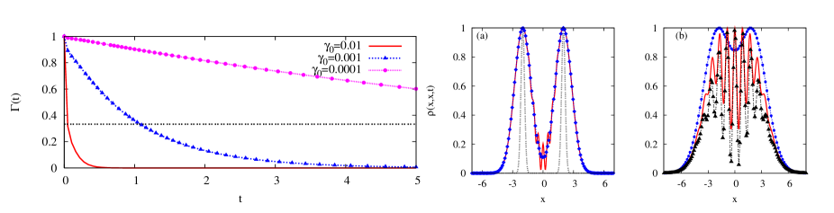
Figure 1: On the left: Evolution in time for the decaying exponential $\Gamma(t)$ that destroys the interferences of the system for different couplings to an environment in the high temperature limit. We use units: $\hbar$ = c = M = 1. Parameters are: $L_{0}=2s^{-1}$, $\sigma_{x0}=0.5s^{-1}$, $k_{B}T=300s^{-1}$. The stronger the coupling to the environment $\gamma_{0}$ is, the sooner decoherence effects take place (for a fixed value of $k_{B}T$ and $L_{0}$). On the right: Interference pattern registered on the screen at a time $t_{L}$ for the closed and open system. In (a), we have considered the case of the isolated subsystem (solid red line) and the case of coupling to a strong environment with $\gamma_{0}=0.01~{}s^{-1}$ (blue dot line). In (b), we have considered three different environments: $\gamma_{0}=0.01~{}s^{-1}$ (blue dot line), $\gamma_{0}=0.001~{}s^{-1}$ (red solid line) and $\gamma_{0}=0.0001~{}s^{-1}$ (black triangle line). Distance is measured in units of frequency.

Clearly, since the decoherence timescale depends inversely on the value of $M\gamma_{0}k_{B}T$, the stronger the coupling to the environment and the hotter the environment, the shorter this timescale.

On the right side of Fig.1, we can see the effects of decoherence on the interference pattern of a thought two-slit interference experiment with particles. In plot (a), we show the interference pattern registered on a screen at a distance $L$ in a time $t_{L}=0.2~{}s$ when the system is closed, i.e. there is no interaction with an environment, and when the system is open. In this latter case, the coupling constant is $\gamma_{0}=0.01$, which represents a strong environment because all interferences have already been destroyed (whereas they are present in the isolated case. In (b), we present a latter time ($t_{L}=0.35~{}s$) for different coupling constants to the environment. We can see that for $\gamma_{0}=0.01~{}s^{-1}$, the two wave packets are spreading and will end up superposing in only one final wave packet since the environment has destroyed the interference in a short timescale. However, for the other two environments, with smaller coupling constants, we can see that the interferences are still there. Notably, the pattern remains unchanged but the visibility is considerably reduced as $M\gamma_{0}k_{B}T$ increases. It is important to note that the visibility is considered attenuated when there is a lost of contrast between a maximum and a minimum with respect to the interference pattern when the system is isolated, i.e. the visibility is reduced when the “minimum” are not exactly zero as seen in Fig.1.

At this stage, it is appropriate to quantify the loss of contrast of the interference pattern. This is done by defining a function called fringe visibility $\nu$, a quantity of particular importance in matter wave interferometry

$$\nu=\frac{I_{\rm max}-I_{\rm min}}{I_{\rm max}+I_{\rm min}},$$

where $I_{\rm max}$ and $I_{\rm min}$ represent the maximum and minimum in neighboring fringes, respectively. It is easy to note that the fringe visibility can be well approximated by

$$\nu(t)\sim\frac{|\rho_{\rm int}(x,x,t)|}{\rho_{11}(x,x,t)+\rho_{22}(x,x,t)},$$

where $\rho_{ii}=|\phi_{i}(x,t)|^{2}$, with $i=1,2$ and $\rho_{\rm{int}}$ the interference terms. The values of this function range between $0$ (no interference fringes) and $1$ (total visibility of the interference fringes). In our case, the visibility fringe can be numerically obtained as

$$\nu(t)\approx\frac{\Gamma(t)}{\cosh(8L_{0}C(t)x)}.$$

Clearly, the visibility fringe goes down as $t_{L}$, i.e. the observation time, is larger than the decoherence time $t_{D}$. However, if we succeed in performing our two slit experiment in a time $t_{L}<t_{D}$ at a fixed room temperature $k_{B}T$, we can see that the visibility fringes depends on $\gamma_{0}$ as shown on the left picture in Fig.2.

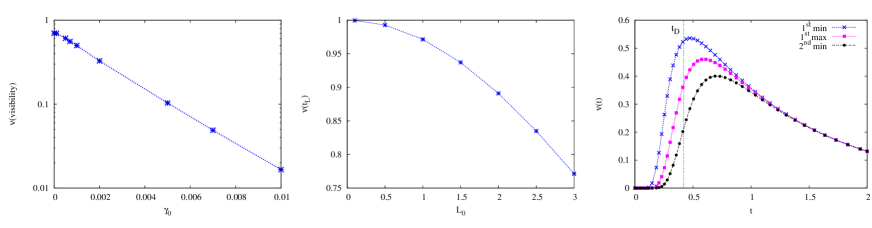
Figure 2: Left: The visibility fringe $\nu(t)$ plotted against $\gamma_{0}$ for a fixed $t_{L}<t_{D}$ at room temperature ($\gamma_{0}$ is in units of frequency). Middle: The visibility fringe $\nu(t)$ as a function of the distance between the slits $L_{0}$ for a fixed time for $k_{B}T=300~{}s^{-1}$, $\gamma_{0}=0.001~{}s^{-1}$, $t_{L}=0.05~{}s$ and $\sigma_{x0}=0.5~{}s^{-1}$. All the decoherence timescales corresponding to the different values of $L_{0}$ (in units of $s^{-1}$) are checked to be longer than $t_{L}$. Right: Time evolution for the visibility fringe $\nu(t)$ for $k_{B}T=300~{}s^{-1}$, $\gamma_{0}=0.001~{}s^{-1}$, $L_{0}=2~{}s^{-1}$ and $\sigma_{x0}=0.5~{}s^{-1}$. The estimation of the decoherence time $t_{D}\sim 1/(M\gamma_{0}k_{B}TL_{0}^{2})=0.41~{}s$ coincides with the timescale at which the visibility starts to decrease towards a null value.

This is so, because the decoherence time depends inversely on the coupling constant. Not only can we check the dependence upon the coupling constant but on the separation of the slits as well.

In the middle of Fig.2, we show the visibility fringe as a function of $L_{0}$. Therein, it is clear that the visibility fringe goes down as the distance between the slits increases. Note that as we are plotting $\nu(t)$ for a fixed value of $t_{L}$ and $\sigma_{x0}$, then we can not vary much $L_{0}$, since we are always assuming that $\sigma_{x0}\leq L_{0}$. We can also study the time evolution of the visibility $\nu(t)$, which is shown on the right side of Fig.2. Therein, we have plotted the evolution in time for the visibility of the first and second minimum and the first maximum of the interference pattern. The behavior exhibited is quite appealing. For short times, the visibility increases from zero to a maximum value because the interferences start to develop at that short timescale but are not present at $t=0$ (since the wave packets are initially separated and have to spread so as to generate the interferences. This maximum value coincides with the estimated decoherence time $t_{D}$. Then, the visibility starts to decrease, since the destruction of the interferences is taking place. Clearly, the decoherence is a dynamic process (the continuous monitoring of the environment over the test particles) and the estimated decoherence time is when the interferences have been reduced about a $70~{}\%$, i.e. $\Gamma(t_{D})\sim 1/e$ (see Fig.1). However, that does not mean that the wigner function will be positive by that time. If one estimates the decoherence time as the one in which the interferences disappear completely, the estimated timescale will be longer and one might naively impute the loss of visibility on another cause but decoherence tumulka . Note that the visibility is a quantity that measures the loss of contrast of the interference fringes. Then, it is expected that those with the bigger contrast suffer from this attenuation the more, as seen in Fig.2. Clearly, the observation time $t_{L}$ must be shorter than the decoherence time in order to observe the interference pattern. The visibility function $\nu(t)$, in this case, tends to zero for longer times.

It shall be interesting to study the visibility function for the other environmental models. In the case of the scattering model, the behavior of $\nu(t)$ as a function of the diffusion term $\Lambda$ and the square of the width of the slit $L_{0}^{2}$ is qualitatively similar to that of the QBM because the expression of $\Gamma_{\Lambda}(t)=\exp(-\Lambda\Delta x^{2}t)$ is formally the same. Then, we expect to find that the visibility decreases as $\Lambda$ and $L_{0}^{2}$ increases, since the decoherence time shall be shorter Pritchard .

Nonetheless, the visibility function for the study of the dephasing effects, i.e. when considering the interaction of the massive particle with the external time dependent electromagnetic field, is not that similar to the other two mentioned throughout the paper. In particular, $\Gamma_{C}=J_{0}(|C|)$ is constant in time as we estimated it in Nos for the experimental data of both neutrons and fullerenes. Therein, we calculated the quantity $C$ for these massive particles and observed that, contrary to might be naively expected, in thought and real experiments such as the one reported in Horn2 , $C_{\rm fullerenes}\sim{\cal O}(1)$. However, for neutral particles with permanent dipole moment this value is much lower $C_{\rm neutrons}\sim{\cal O}(0.01)-{\cal O}(0.1)$. Therefore, on the left side of Fig.3 we present the time evolution of the visibility function $\nu_{C}(t)$ defined as

$$\nu_{C}(t)=\frac{J_{0}(|C|)}{\cosh(8L_{0}C(t)x)}.$$

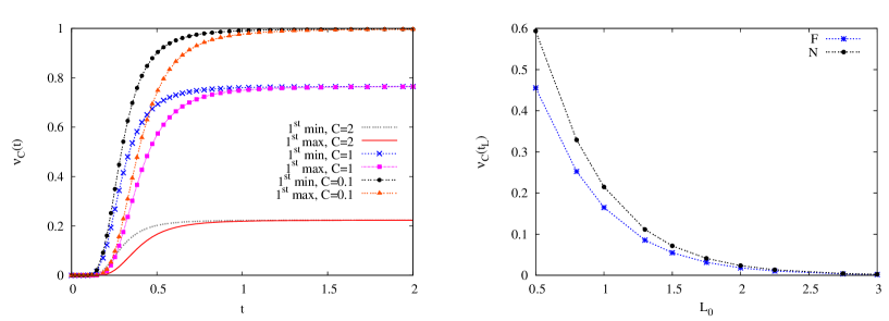
Figure 3: Left: Time evolution for the visibility function $\nu_{C}(t)$ for neutrons ($C_{\rm neutrons}=0.1$) and fullerenes ($C_{\rm fullerenes}=1$ and $C_{\rm fullerenes}=2$) in the presence of an external time dependent electromagnetic field. The curves are for the first minimum and maximum of the interference pattern. We can see that all curves reach an asymptotic limit that is not zero contrary to the other two environmental models (see Fig.2). Right: The visibility fringe $\nu_{C}(t)$ as a function of the separation of the slits $L_{0}$ for a fixed time for time $t_{L}=0.20~{}s$, $t_{L}=0.05~{}s$ and $\sigma_{x0}=0.5~{}s^{-1}$. The curves shown are for the first maximum of the interference pattern in the case of neutrons and fullerenes. $L_{0}$ is in units of $s^{-1}$.

Therein, we show the time evolution of the first maximum and minimum of the interference pattern for different values of the $C$ factor. It is easy to note that the development of the interferences happens in the same timescale of Fig.2 (for the same value of $L_{0}$ and $\sigma_{x0}$) but in all cases, reach a different asymptotic value compared to the $\nu(t)$ function. The fact that $\nu_{C}(t)$ has an asymptotic limit could really be of much use in experiments where this effect is of importance, such as fullerenes, since once this limit is reached the observation time $t_{L}$ can be any subsequent time for the visibility function remains steady.

Another feature of this visibility function $\nu_{C}(t)$ worth of studying is its dependence upon the separation of the slits $L_{0}$. On the right side of Fig.3 we present this behavior. Clearly, the behavior exhibited therein is qualitatively different from that showed in Fig.2 for the visibility function $\nu$ with $\Gamma_{\cal D}(t)$.

Finally, in Fig.4, the interference pattern for the experimental data reported in Horn2 for two-slit experiments with massive particles $C_{70}$ is shown. Therein, we have considered the unitary and non unitary evolution (for the three environmental models $\Gamma_{\cal D}(t)$, $\Gamma_{\Lambda}(t)$ and $\Gamma_{C}$) of the particles. For these massive particles, we can see that the interference pattern is always attenuated when the system is open. What is more significant, is that the effect of $\Gamma_{C}$ can be as important as the other two most widely known model environments (in agreement with tumulka but using a different model for dephasing) and enough to model the real experiment. For the values of Fig.4, and asking $t_{D}>t_{L}$ (and correspondingly $t_{\Lambda}>t_{L}$), we obtain a constraint for the free parameters of each model: $\gamma_{0}<7.14\times 10^{-8}~{}[\rm{s^{-1}}]$ (as estimated in Venugopalan ) and $\Lambda<7.44\times 10^{15}~{}[\rm{m^{-2}s^{-1}}]$ (approximately the value used in Viale ) for the experimental data at room temperature reported in Horn2 .

We want to emphasize that Eq.(3) phenomenologically models the decoherence effects neglecting the dissipative process. The value we obtained for $\gamma_{0}$ is extremely small so a valid question might be if it is necessary to include dissipation in the model. We state that it positively is in order to have a complete and formally correct description of the process. By including the term proportional to $\gamma(t)$ in Eq.(5) we are assuring the fulfilment of the fluctuation-dissipation theorem, also known as Einstein formula in the high temperature limit. It is known that the diffusive coefficient ${\cal D}=2M\gamma_{0}k_{B}T$ is proportional to $\gamma_{0}$. In this way, if $\gamma_{0}$ happens to be zero (which means no dissipation), the diffusive term would also be zero. The correctness of the formulation can also be checked in the fact that even though $\gamma_{0}$ is extremely small, $M\gamma_{0}k_{b}T$ can be very large. In such a case, the decoherence effects would be very important whereas the dissipative interaction between the particles and the environment can be ignored. In other words, small dissipation implies that the particles could have a neglible damping term in the semiclassical Langevin equation of motion along the ${\hat{x}}$ direction, but the existance of noise ensures that decoherence shall be effective.

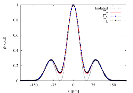
Figure 4: The interference pattern ($\nu\sim 0.68$) registered on the screen for the unitary evolution and the nonunitary evolution considering the different model environments for a double slit diffraction experiment with massive particles $C_{70}$. The curves are done with the experimental data reported in Horn2 . The values used for the plot: $\gamma_{0}=2.6\times 10^{-8}~{}s^{-1}$, $\Lambda=2.8\times 10^{15}~{}s^{-1}$ and $C=1$.

It is important to stress that all these environmental models consider one and only one “decoherent” agent influencing the interference experiment. However, all these effects can be together considered to be present in a two-slit experiment. In such a case, the attenuation factor $\Gamma$ would be $\Gamma\approx\Gamma_{\Lambda}+\Gamma_{{\cal D}}+\Gamma_{C}$. The effect of the environment would be equal to the sum of the three factors (as seen in Fig.4). Therefore, it is enough to consider the biggest one (unless they are all the same order of magnitude). All in all, it is necessary to remark that decoherence effects do play a crucial role in the fringe visibility reduction. On the one hand, authors in tumulka said that the incoherence of the source was to blame for the fringe visibility reduction. On the other hand, authors in Sanz developed a phenomenological theoretical model where decoherence was a priori introduced by assuming an exponential damping of the interferences. So far, we have shown that the scattering of the massive particles with the air molecules and dephasing (for example introduced by the random emission time) of the experimental setup are all responsible for the fringe visibility reduction and approximately of the same order of magnitude.

IV Application: Experimental Data for Neutrons

In this Section, we shall use the existing experimental data Nairz ; Zeilinger to reproduce the observed patterns for neutral cold atoms.

If we consider that $t_{L}=L/v=M\lambda_{\rm dB}L/(2\pi\hbar)$ and $t_{L}>>M\sigma_{x0}L_{0}/\hbar$, then the position distribution on the screen at this time $t_{L}$ can be well approximated by:

$$P(x,t_{L})=\frac{8\pi\sigma_{x0}^{2}N^{2}}{\lambda_{\rm dB}L}\exp\bigg{\{}-\bigg{(}\frac{2\sqrt{2}\pi\sigma_{x0}x}{\lambda_{\rm dB}L}\bigg{)}^{2}\bigg{\}}\times\bigg{[}1+\Gamma(t_{L})\cos\bigg{(}\frac{2\pi L_{0}x}{\lambda_{\rm dB}L}\bigg{)}\bigg{]},$$ (9)

where $\Gamma(t_{L})$ depends on the model environment we want to use to describe the conditions in which the two-slit experiment is being done evaluated in the observation time. In this way, Eq.(9) describes the intensity on the screen as a function of the experimental parameters, i.e, the mass $M$ of the cold neutrons, the associated wavelength $\lambda_{\rm dB}$, the distance to the screen $L$, the distance between the slits $L_{0}$ (assuming the two slits are as similar as possible) and the initial width of the wave packet $\sigma_{x0}$. All these values can be found, for example, in Sanz for cold neutrons. Note that Eq.(9) is equivalent to Eq.(8) , identifying our time dependent theoretical parameters with the real experimental ones. Thus, we have for a fixed observational time $t_{L}$ (making the same assumptions as in the above section)

$$B(t_{L})=\frac{2\pi}{\lambda_{\rm dB}L}~{}~{}~{}{\rm and}~{}~{}~{}C(t_{L})=\bigg{(}\frac{2\sqrt{2}\pi\sigma_{x0}}{\lambda_{\rm dB}L}\bigg{)}^{2}.$$

In the case we studied in the preceeding Section, assuming that the dynamics of the test particle can be modeled by a quantum brownian motion, the expression for $\Gamma(t_{L})$ is $\Gamma_{D}(t_{L})=\exp(-t_{L}/t_{D})$ with $t_{D}=12\hbar^{2}/(M\gamma_{0}k_{B}TL_{0}^{2})$ where we have reincorporated $\hbar$. In the estimation of this time we have considered that $\Delta x^{2}\sim L_{0}^{2}$, which in fact is an underestimation of the decoherence time for lengths bigger than $L_{0}$. As the experiment is done at room temperature, the only free parameter is the value of $\gamma_{0}$. On the other hand, if the model environment were assumed to be the one of the scattering with air molecules, where the effects of the environment are included in the collision term $\Lambda$, then the expression for $\Gamma(t_{L})$ would be $\Gamma_{\Lambda}(t_{L})=\exp(-t_{L}/t_{\Lambda})$ with $t_{\Lambda}=3/(\Lambda L_{0}^{2})$.

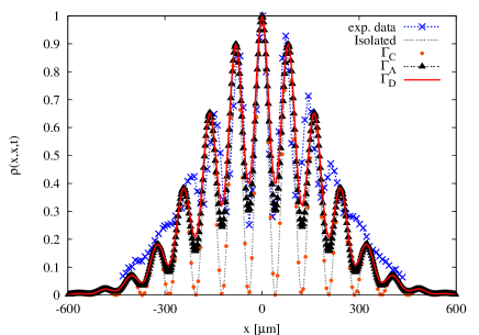
Figure 5: The interference pattern ($\nu\sim 0.57$) registered on the screen for the unitary evolution and the nonunitary evolution considering the different model environments. Experimental results obtained by Zeilinger et. al Zeilinger2 for the double slit diffraction of cold neutrons are plotted with blue star dots. The values used for the plot: $\gamma_{0}=5.0\times 10^{-12}~{}s^{-1}$ , $\Lambda=5.5\times 10^{11}~{}s^{-1}$.

The other possible environmental model mentioned in Sec.II.2 was to considered the interaction with the charged or neutral (with permanent dipole moment) particles with the electromagnetic field. This is an interaction that is always present, can never be turned off, although sometimes it is possible to neglect it. As we previously studied in Nos , in the case of neutral particles with permanent dipole moment, this effect is not so important.

In Fig.5 we have plotted, the interference pattern for the experimental data reported for experiments with cold neutrons for the isolated and open system. In this last case, the nonunitary evolution has been considered for the different environment models mentioned above. We can clearly see, that for this case, the nonunitary evolution when considering the interaction of the cold neutrons with a time-varying electromagnetic field (orange dots) is exactly superposed with the unitary one (dotted line). That means that the incoherence effects can be completely neglected. However, the other two model environments, whose effects are considered in $\Gamma_{\Lambda}(t)$ (black triangle dotted line) and $\Gamma_{D}(t)$ (red solid line), fit correctly the experimental data obtained by Zeilinger et al. (blue star dotted line) in Zeilinger2 . The fact that the interference pattern is observed implies that the decoherence time is $t_{D}$ (and $t_{\Lambda}$) is larger than the observation time $t_{L}$. That sets us a constraint to the expected values for $\gamma_{0}$ (and $\Lambda$), the free parameter in each model. By asking $t_{D}>t_{L}$, we have $\gamma_{0}<8\times 10^{-9}~{}[s^{-1}]$. In the case of modeling the environment by a collision term $\Lambda$, if $t_{\Lambda}<t_{L}$ is asked, then $\Lambda<1.28\times 10^{14}~{}[\rm{m^{-2}s^{-1}}]$.

V Final Remarks

The effect of the environment on the interference pattern of a two-slit interference experiment with massive particles has been studied phenomenologically in the literature.

However, here we have presented a fully quantum mechanical treatment using a microscopic model of environment and also a concrete example to include dephasing effects. Therefore, we have studied the effects of decoherence on the interference pattern of thought experiments and presented an analysis of matter wave interferometry in the presence of a dynamic quantum environment such as the quantum brownian motion model. We have shown the interference patterns and visibility function $\nu(t)$ for thought diffracted free particles and analyzed their dependence upon different parameters of the model in the high temperature limit (assumption valid for massive particles interfering at room temperature). As was expected, the visibility decreases as the value of the diffusion coefficient increases and, in particular, we showed this effect for different values of the coupling constant $\gamma_{0}$ to the environment. What is more important, we have seen that the visibility fringe is considerably reduced when considering an open quantum system, although the structure of the interference pattern remains unchanged.

Yet more important, we defined the visibility function $\nu_{C}$ for a model environment previously developed which describes dephasing effects originated in the experimental difficulty of producing the same initial/final state for all particles (i.e the existence of a random variable such as the particle’s emission time). We showed that it is qualitatively different than the one commonly found in the literature and very important in the case of experiments with massive particles such as fullerenes. In this case, dephasing effects are enough to model the attenuation of the interference pattern observed in the real experiment, whereas in the case of cold neutrons these effects are not of such importance. Therefore, in the latter case we must consider the decoherence effects by using the corresponding formulation. This result might have been expected since the interaction of more massive particles with the external classical field is more important than for those with a smaller mass where other kind of interactions seem to prevail.

Finally, the effect of the environment on a two-slit experiment can be modeled by considering different effects such as the scattering of the massive particles with the air molecules, the randomness of the arrival or emission times and the presence of a classical time dependent electromagnetic field. Even though there exist conceptual differences in all the cases mentioned throughout the paper, we showed that all these effects reduce the visibility fringe and can be formally deduced from a microscopic model (whether the QBM for decoherence effects studied in this paper or a fluctuating Aharonov-Casher phase studied in our previous contribution). They are all included in the noise induced effects introduced in the subsystem when the latter is coupled to a quantum external environment.

VI Acknowledgments

This work was supported by UBA, CONICET, Fundación Antorchas, and ANPCyT, Argentina. Authors gratefully acknowledge A.S.Sanz for sending the experimental data for neutrons. Paula I. Villar gratefully acknowledges financial support of UIPAP.

References

- (1) P. Facchi, S. Pascazio and T. Yoneda , (2005). Preprint quant-ph/0509032
- (2) B. Brezger, L. Hackermuller, S. Uttenthaler, J. Petschinka, M. Arndt and A. Zeilinger, Phys. Rev. Lett. 88, 100404 (2002).
- (3) K. Hornberger, S. Uttenthaler, B. Brezger, L. Hackermuller, M. Arndt, and A. Zeilinger Phys. Rev. Lett. 90, 160401 (2003).
- (4) W. Zurek, Rev. Mod. Phys. 75, 715 (2003).
- (5) R.E. Grisent, W. Schöllkopf, J.P. Toennies, G.C. Hegerfeldt, and T. Köhler, Phys. Rev. Lett. 83, 1755 (1999).
- (6) M. Bozic, D. Arsenovic, and L. Vuskovic, Phys. Rev. A69, 053618 (2004).
- (7) A. Stern, Y. Aharonov, and Y. Imry, Phys. Rev. A41, 3436 (1990).
- (8) A. S. Sanz, F. Borondo and M. J. Bastians, Phys. Rev. A 71, 042103 (2005).
- (9) T. Qureshi, and A. Venugopalan, to be published in Int. J. Mod. Phys. B (2007); quant-ph/0602052.
- (10) R. Tumulka, A. Viale, and N. Zanghi, quanth-ph/0608021.
- (11) A. Viale, M. Vicari, and N. Zanghi, Phys. Rev. A 68, 063610 (2003).
- (12) D. Giulini, E. Joos, C. Kiefer, J. Kupsch, I.O. Stematescu, and H.D. Zeh, Decoherence and the Appearance of a Classical World in Quantum Theory, Springer, Berlin (1996).
- (13) D.F. Walls and G.J. Milburn, Phys. Rev. A31, 2403 (1985).
- (14) L. Diosi, Europhys. Lett. 30, 63 (1995).
- (15) B. Vacchini, Phys. Rev. Lett. 84, 1374 (2000).
- (16) B. Vacchini, Phys. Rev. E63, 066115 (2001).
- (17) M.R. Gallis and G.N. Fleming, Phys. Rev. A42, 38 (1990).
- (18) D. Kokorowski, A.D. Cronin, T.D. Roberts, and D.E. Pritchard, Phys. Rev. Lett. 86, 2191 (2001).
- (19) K. Hornberger, J.E. Sipe, and M. Arndt, Phys. Rev. A 70, 053608 (2004).
- (20) K. Hornberger, Phys. Rev. Lett. 97, 060601 (2006).
- (21) K. Hornberger, Phys. Rev. A73, 052102 (2006).
- (22) F. C. Lombardo, F. D. Mazzitelli, and P. I. Villar, Phys. Rev. A 72, 042111 (2005); F.C. Lombardo and P.I. Villar, J. Phys. A. 39, 6509-6516 (2006).
- (23) B. Hu, J.P. Paz, and Y. Zang, Phys. Rew. D 45, 2843 (1992).
- (24) D. Gobert, J. von Delft, and V. Ambegaokar, Decoherence without dissipation?; quant-ph/0306019.
- (25) J. Bernabeu, N.E. Mavromatos, and S. Sarkar, Pĥys. Rev. D74, 047014 (2006).
- (26) B. Lamine, R. Hervé, A. Lambrecht, and S. Reynaud, Phys. Rev. Lett. 96, 050405 (2006).
- (27) F.C. Lombardo and P.I. Villar, Phys. Rev. A74, 042311 (2006).
- (28) F.C. Lombardo and P.I. Villar, Phys. Lett. A 336, 16 (2005).
- (29) N.Antunes, F.C. Lombardo, D. Monteoliva, and P.I. Villar, Phys. Rev. E73, 066105 (2006).
- (30) O. Nairz, M. Arndt and A. Zeilinger, J. Mod. Opt. 47, 2811 (2000).
- (31) A. Zeilinger et al., Rev. Mod. Phys. 60, 1067 (1988).
- (32) A. Zeilinger, R. Gahler, W. Treimer, and W. Mampe, Rev. Mod. Phys. 60, 1067 (1988).