The UV Continuum of Quasars: Models and SDSS Spectral Slopes

Abstract

We measure long (2200-4000 Å) and short (1450-2200 Å) wavelength spectral slopes $\alpha$ ($F_{\nu}\propto\nu^{\alpha}$) for quasar spectra from the Sloan Digital Sky Survey. The long and short wavelength slopes are computed from 3646 and 2706 quasars with redshifts in the z=0.76-1.26 and z=1.67-2.07 ranges, respectively. We calculate mean slopes after binning the data by monochromatic luminosity at 2200 Å and virial mass estimates based on measurements of the Mg II line width and 3000 Å continuum luminosity. We find little evidence for mass dependent variations in the mean slopes, but a significant luminosity dependent trend in the near UV spectral slopes is observed with larger (bluer) slopes at higher luminosities. The far UV slopes show no clear variation with luminosity and are generally lower (redder) than the near UV slopes at comparable luminosities, suggesting a slightly concave quasar continuum shape. We compare these results with Monte Carlo distributions of slopes computed from models of thin accretion disks, accounting for uncertainties in the mass estimates. The model slopes produce mass dependent trends which are larger than observed, though this conclusion is sensitive to the assumed uncertainties in the mass estimates. The model slopes are also generally bluer than observed, and we argue that reddening by dust intrinsic to the source or host galaxy may account for much of the discrepancy.

1. Introduction

The “bare” thin accretion disk has been invoked ubiquitously to explain both general and detailed properties of a wide variety of accreting systems. In systems which are believed to harbor black holes the results have been mixed. The timing and spectral variations of Galactic black hole candidates show a range of behavior, much of which cannot be accommodated by a simple thin accretion disk. However, some of these sources enter a thermal state, where the spectral energy density (SED) is dominated by emission which can be well fit with a simple multitemperature blackbody model (Mitsuda et al., 1984) or more elaborate variations (e.g. Li et al., 2005; Davis & Hubeny, 2006).

The thin disk model may also explain a portion of the emission in Active Galactic Nuclei (AGNs). These sources are almost certainly powered by an accretion flows onto a central “super-massive” black hole (Krolik, 1999). As a result, it is often supposed that the broad UV peak (“big blue bump”) of the SED is emission from a thin accretion disk. However, this interpretation faces a number of challenges when detailed comparisons are made between models and the data (see e.g. Koratkar & Blaes, 1999). It may be possible to resolve some of these discrepancies by modifying the model and considering additional processes (e.g. dust reddening, irradiation, inhomogeneities, and multi-phase flows), but it is then pertinent to ask what, if any, predictive power is provided by the thin disk model itself.

Models of thin accretion disks predict that the effective temperature at the inner-most radius $T_{\rm in}$ of the disk will be proportional to the one-fourth power of accretion rate $\dot{M}$ and inversely proportional to one-half power of black hole mass $M$ ($T_{\rm in}^{4}\propto\dot{M}/M^{2}$). This scaling follows rather generally from the assumptions that gravitational binding energy is radiated locally and that the relevant length scale of the emitting region is the gravitational radius $R_{g}=GM/c^{2}$ of the black hole. As we shall discuss, this relation accounts for much (but not all) of the spectral dependence on $M$ and $\dot{M}$ since $T_{\rm in}$ roughly determines the photon energy where the SED peaks ($\sim k_{\rm B}T_{\rm in}$).

In fact, one of the successes of this scenario is that it approximately predicts the position of the continuum peak for both super-massive black holes in AGN and the $\sim 10M_{\odot}$ black holes in Galactic X-ray binaries, assuming that both sources accrete mass at similar fraction of the Eddington limit. Also, the approximate relation $T_{\rm in}^{4}\propto L\propto\dot{M}$ (where $L$ is the bolometric luminosity) can be inferred from the spectral evolution of several black hole binaries in thermal state (see e.g. Gierliński & Done, 2004). Unfortunately the narrow range of dynamically inferred masses, uncertainties in the estimates, and small sample of sources complicate efforts to simultaneously and independently constrain the $M$ dependence of the SED in these systems.

In many respects, AGNs offer greater promise for testing the $M$ and $L$ (or $\dot{M}$) dependence of thin disk spectral models since there is a much larger sample available which spans a wider range of $M$ and $L$. However, there are also a number of additional challenges. First, mass estimates in AGN are generally more uncertain than in black hole candidates, and the most reliable methods can only be applied in a small fraction of sources. Also, the SED peaks in the far UV so it is challenging to get broadband coverage at low redshifts, except for a relatively small number of bright sources. Finally, the large number of emission lines which characterize most AGN may prevent a robust determination of underlying continuum emission.

Despite these challenges, comparing the predicted and observed spectral evolution as a function of $M$ and $L$ is the principle aim of this work. To accomplish this, we measure UV spectral slopes ($\alpha$ where $F_{\nu}\propto\nu^{\alpha}$) for several thousand quasars from the Sloan Digital Sky Survey (SDSS). A wide range of $\alpha$ is inferred, allowing us to examine the extent to which $\alpha$ correlates with the $M$ and $L$, the parameters which determine the model SEDs (see e.g. Sun & Malkan, 1989; Laor & Netzer, 1989; Hubeny et al., 2000). We compare the observed slopes with calculations based on the relativistic, fully non-LTE models of Hubeny et al. (2000). In addition to allowing us to test the predictions of the thin disk model, a correlation (or lack thereof) may provide clues and place important constraints on other processes which may be important for determining the continuum SED.

The plan of this work is as follows. In order to test the predictions of the thin disk model we construct a large table of artificial SEDs for direct comparison with data. The methods used to construct these models are summarized in §2. In §3.1 we briefly review the mass estimation methods employed in this work as our conclusions are sensitive to the reliability of these estimates. In §3.2 we compare the model SEDs with a small sample of well-observed, relatively nearby AGNs with simultaneous optical to UV spectra (Shang et al., 2005). In §4 we present slope measurements for a large sample of SDSS QSOs. In §5 we calculate slopes from our spectral models and generate Monte Carlo realizations of the slope distributions for comparison with the data. In §6 we discuss the possible origins of discrepancies between the models and observations, considering additional processes, not accounted for by the models, which might be important. In §6.4, we compare our results with previous work, particularly that of Bonning et al. (2006) which is the most similar to our current efforts. We summarize our conclusions in §6.5. Throughout this work, we use the following cosmology: $H_{0}=70\;{\rm km\;s^{-1}\;Mpc^{-1}}$, $\Omega_{m}=0.3$, and $\Omega_{\Lambda}=0.7$.

2. Spectral Models

Our artificial SEDs are based on time-independent models of thin, $\alpha$-disks (Shakura & Sunyaev, 1973). Here, $\alpha$ refers to an assumed constant of proportionality between the accretion stress and total pressure. Therefore, it is a dimensionless parameter and generally assumed to be less than unity. (Hereafter, we will use $\alpha_{\rm SS}$ to differentiate this quantity and the spectral slope $\alpha$, but we will continue to refer to the model simply as an $\alpha$-disk.) We generate artificial SEDs using AGNSPEC, an interpolation scheme which is identical to that described in Davis & Hubeny (2006). Except for the interpolation scheme, the models used here are equivalent to those presented in Hubeny et al. (2000). We only summarize the most relevant features and the reader is referred to this work (and references therein) for a more detailed discussion.

The artificial SEDs are based on a relativistic, thin, $\alpha$-disk model similar to that of Novikov & Thorne (1973), but include some minor corrections (Riffert & Herold, 1995). These SEDs account for the effects of light bending and time dilation by calculating the null geodesics of the black hole spacetime (KERRTRANS, Agol, 1997). In addition to $M$ and $\dot{M}$, such fully-relativistic models require a choice of the black hole spin parameter $a_{\ast}=cJ/GM^{2}$, where $J$ is the angular momentum of the hole.

Using these “one-zone” disk models as a basis, we compute two types of artificial SEDs. We first construct relatively simple spectra which assume the disk surface emits like a blackbody at the local effective temperature (but still account for relativistic effects). A second set of more sophisticated models employ TLUSTY (Hubeny & Lanz, 1995) to solve the coupled equations of radiative transfer and equilibrium, non-LTE vertical structure in the disk. In this case the disk surface density is needed to determine the structure, requiring a model for angular momentum transport. We adopt an $\alpha$-disk prescription with $\alpha_{\rm SS}=0.01$. At the wavelengths of interest the spectra are relatively insensitive to $\alpha_{\rm SS}$ for the ranges of parameters ($a_{\ast}$, $M$, and $L$) explored here. These models include bound-free and free-free opacities of H and He and the effects of electron scattering are calculated in the Thomson limit. Due to the difficulties involved, we do not include opacity from bound-bound transitions, although it may have a significant effect on the resulting spectra (see e.g. Hubeny & Hubeny, 1998).

The inclusion of non-LTE effects and realistic opacities can cause significant shifts from a simple blackbody spectrum. The effects are usually largest at frequencies near the bound-free transitions. Since we concentrate on the SED at wavelengths longer than 1000 Å, the Balmer edge will be the most important. Unfortunately, the annuli which produce most of the flux longward of the Balmer edge are the most difficult to calculate due the presence of ionization zones associate with the transition. In these annuli, equilibrium solutions are either unattainable or lead to unstable atmospheres with density inversions (see §3.3 of Hubeny et al., 2000). Due to these difficulties, we simply assume blackbody spectra for annuli with effective temperatures below 9,000 K. Based on Fig. 11 of Hubeny et al. (2000), this probably leads to a slight underestimate of flux at 4000 Å and possible implications are discussed in §6.3.

3. Methods

3.1. Mass Estimates

Table 1Slope Comparison

Source	Mass	$\alpha(1450-2200{\rm\AA})$			$\alpha(2200-4000{\rm\AA})$			$\alpha(1450-4000{\rm\AA})$
	($10^{8}M_{\odot}$)	Data	$a=0$	$a=0.9$	Data	$a=0$	$a=0.9$	Data	$a=0$	$a=0.9$
3C 273	8.86	-0.64	-0.34	-0.24	0.08	-0.16	-0.11	-0.21	-0.23	-0.16
PG 0953+414	2.76	-0.16	-0.17	-0.12	-0.27	-0.12	-0.080	-0.23	-0.14	-0.095
PG 0052+251	3.69	-0.60	-0.21	-0.038	-0.28	-0.28	-0.14	-0.41	-0.25	-0.097
Ton 951	0.92	-0.98	0.00	0.073	-0.57	-0.14	-0.074	-0.74	-0.08	-0.014
Mrk 509	1.43	-1.0	-0.074	0.092	-0.19	-0.24	-0.096	-0.52	-0.17	-0.019

Stellar dynamical estimates of black hole masses are only available in the local universe. At higher redshifts virial mass estimates based on reverberation mapping of broad line region (BLR) clouds (see e.g. Peterson et al., 2004) are generally accepted to be the most reliable (see, however, Krolik, 2001). This technique uses the full-width-at-half-maximum (FWHM) or second moment of one or more prominent broad emission lines to estimate the velocity field $v_{\rm BLR}$ of broad line clouds. Reverberation mapping then provides a characteristic radius $R_{\rm BLR}$ from which the virial mass $M_{\rm vir}\sim v_{\rm BLR}^{2}R_{\rm BLR}/G$ can be estimated. The precise normalization depends on the kinematics of the BLR and cannot, in general, be determined reliably for individual sources. A single normalization for all sources can be obtained by requiring virial estimates to lie on the $M-\sigma$ relation (Onken et al., 2004).

A significant drawback of this method is that it requires sources to be frequently monitored and can only be robustly applied in cases where the lines provide a clear response to continuum variations. As a result, it has only been used successfully for relatively nearby sources. (Wandel et al., 1999; Kaspi et al., 2000, 2005). At higher redshifts, empirically calibrated luminosity–radius relations are more commonly used (e.g. Vestergaard, 2002; Woo & Urry, 2002; Vestergaard & Peterson, 2006). For these methods it is generally assumed that $R_{\rm BLR}\propto(\lambda L_{\lambda})^{\delta}$ where monochromatic luminosity $\lambda L_{\lambda}$ is calculated at some particular rest wavelength. This is usually chosen to be 5100 Å when $v_{\rm BLR}$ is estimated from the width of H$\beta$. The constant of proportionality and exponent $\delta$ are then fit to minimize the scatter between this relation and estimates from a reverberation mapped sample. Typically $\delta\sim 0.5$ (see e.g. Bentz et al., 2006) is obtained, consistent with expectations from photoionization models of the BLR.

At higher redshifts, H$\beta$ shifts out of the observed band and other broad emission lines are used, typically Mg II or C IV. The estimates used in §4 were calculated from line width measurements obtained by McLure & Dunlop (2004) and the reader is referred to their paper for a detailed discussion. Since we are only considering quasars with $z\gtrsim 0.7$ all estimates utilize the FWHM of Mg II $v_{\rm Mg}$ and $L_{3000}$ the monochromatic luminosity measured at 3000 Å. Therefore, the mass estimates are calculated using equation (A6) of McLure & Dunlop (2004)

$$\frac{M_{\rm vir}}{M_{\odot}}=3.2\left(\frac{L_{3000}}{10^{44}{\rm\;erg\;s^{-1}}}\right)^{\delta}\left(\frac{v_{\rm Mg}}{\rm km\;s^{-1}}\right)^{2}.$$ (1)

Using $L_{3000}$, McLure & Jarvis (2002) obtain $\delta=0.47$ by fitting the $R_{\rm BLR}-L_{3000}$ relation to best match reverberation mapped masses of 34 AGNs (Kaspi et al., 2000). However, this relation is derived including a number of relatively low luminosity AGNs while the $z>0.7$ SDSS quasar sample only includes sources with $L_{3000}>10^{44}\rm\;erg\;s^{-1}$. Therefore, McLure & Dunlop (2004) refit the $R_{\rm BLR}-L_{3000}$ relation only using those sources in the reverberation mapped sample with $L_{3000}>10^{44}\rm\;erg\;s^{-1}$, finding $\delta=0.62$. Since our sample is a subset of the McLure & Dunlop (2004) sample which only includes this luminosity range, we also adopt the $\delta=0.62$ value.

Figure 1.— Optical to UV SEDs of five AGN from the sample of Shang et al. (2005). The dashed curves are model SEDs with $M$ corresponding to the the reverberation mapping estimates in Table 1 and $a_{\ast}=0$. We choose the inclinations $i$ so that $\cos i=0.8$ for all models except 3C 273. In this case we use $\cos i=1$ since the source exhibits superluminal motion. The accretion rate is fixed by approximately matching the model and data at 4000 Å. In Ton 951 and Mrk 509 the bare models are clearly a poor approximation so we also consider models (dotted covers) which are reddened using an SMC-like extinction curve. See the text in §3.2 for further discussion.

3.2. Comparing Models to Data with Spectral Slopes

One of the most striking characteristics of most AGNs (particularly quasars and type I Seyferts) are the numerous strong broad, emission lines. A substantial fraction of the UV and optical flux can be emitted in these lines, making a precise and robust identification of the continuum difficult, if not impossible. In some cases the broad line region emission appears to be unpolarized and the underlying continuum can be identified with polarimetry (Kishimoto et al., 2003, 2004), revealing a Balmer edge beneath the “small blue bump”. Although promising, this technique requires polarimetry observations and unpolarized BLR emission, making it unsuitable for our purposes. Alternatively, we could attempt to model the BLR emission. Photoionization models can qualitatively reproduce many aspects of the observed spectra, but detailed fits to individual SEDs remain a challenge. Therefore, we feel the substantial work involved in generating such models and fitting the data is best left for future efforts.

Lacking a suitable method for removing the BLR emission, we simply adopt “continuum windows” which appear to be largely devoid of BLR contamination and focus on the flux at these wavelength for comparison with the models. Unfortunately, no part of the spectrum is completely devoid of line emission, and the best one can hope to do is choose regions which are relatively free of BLR contamination. Our choices are guided in part by the SDSS quasar composite of Vanden Berk et al. (2001). By constructing a composite spectrum from thousands of quasars, one can construct a high signal-to-noise SED which is sensitive to the presence of rather weak emission features. We focus on three windows near 1450 Å, 2200 Å, and 4000 Å.

In making these choices, we have attempted to balance the requirement of little contamination with a desire to have as large a sample of quasar spectra as possible which cover two of the windows. Of these choices, 2200 Å is probably the most problematic due to the presence of Fe II contamination (see e.g. Fig. 6 of Vanden Berk et al., 2001). However, there are no preferable options between 1450 Å and 4000 Å. The SDSS spectra cover an observed wavelength range from 3800 Å to 9200 Å, roughly a factor 2.4. Therefore, 1450 Å and 4000 Å cannot be simultaneously covered with SDSS, making an intermediate window necessary.

Although we do not have full UV spectral coverage for the SDSS quasars, we can gain insight by first comparing our models with broadband spectra of lower redshift AGN. The sample of Shang et al. (2005) is ideally suited for this purpose. It combines nearly simultaneous spectra for 17 relatively bright, nearby AGN taken with Far Ultraviolet Spectroscopic Explorer, Hubble Space Telescope, and the 2.1 m Kitt Peak National Observatory. Shang et al. (2005) provide a detailed analysis of the sample, including comparisons with the spectral models described in §2. Here we only provide a brief comparison of five sources with reverberation mapping mass estimates (Peterson et al., 2004).

As shown in Figure 1, the SEDs of these sources were shifted to rest wavelength and corrected for Galactic reddening using the values from Table 1 of Shang et al. (2005) which were obtained from NED and based on the Schlegel et al. (1998) map. The centers of the continuum windows are marked with dashed vertical lines. For comparison we plot thin disk models for $a_{\ast}=0$ black holes as dashed curves. The models can be very roughly approximated by power laws except for the breaks near the Lyman and Balmer edges at 912 Å and 3650 Å. The broad feature between 2200 Å and 4000 Å (“small blue bump”) is predominantly a superposition of Balmer continuum and a plethora of Fe II emission lines produced by the BLR, and, therefore, not accounted for by the model SEDs.

The black hole masses used for the models are equivalent to the reverberation mapping estimates which are listed in the second column of Table 1 (Peterson et al., 2004). The model $\dot{M}$ is chosen to approximately match the observed flux at 4000 Å, assuming an inclination $i$ such that $\cos i=0.8$ for all cases except 3C 273. In the case of 3C 273, we used $i=0$ since superluminal motion is observed in this source. The model bolometric luminosities in Eddington units are 0.32, 0.63, 0.063, 0.16, and 0.035 for 3C 273, PG 0953+414, PG 0052+251, Ton 951, and Mrk 509, respectively.

Qualitatively, the comparisons provide mixed results. They are somewhat better for the higher luminosity AGN, but the the model spectra are clearly too steep in the UV for the lowest luminosity sources (Ton 951 and Mrk 509). PG 0953+414 and PG 0052+251 yield the best results in 1450-4000 Å band, although they respectively overpredict and underpredict the emission below 1000 Å. Although the model provides an approximate reproduction of the continuum in 3C 273 for $\lambda\lesssim 1450$ Å and $\lambda\gtrsim 4000$ Å, it clearly underestimates the flux at 2200 Å. In PG 0052+251, Ton 951, and Mrk 509, the models clearly underestimate optical continuum. We attribute some fraction of this discrepancy to contamination from the host galaxy. This conclusion is supported by the apparent anticorrelation between the optical “excess” and AGN luminosity as the fractional contamination should be weaker in the more luminous AGN if we assume an approximately constant host contribution.

Intrinsic reddening due to dust in the host galaxy may contribute to some of the discrepancy between data and models in Ton 951 and Mrk 509. However, there is disagreement about the form of the reddening curve in QSOs, an issue we discuss further in §6.1. As an example, we plot models (dotted curves) which have been reddened with the “SMC-like” reddening curve (Prevot et al., 1984) $A_{\lambda}=1.39\;E(B-V)(\lambda/\mu{\rm m})^{-1.2}$ adopted by Richards et al. (2003). We adjust E(B-V) and $\dot{M}$ in an attempt to obtain good agreement at 1450 Å and 2200 Å, but still require the flux to match the observed value at 4000 Å. We find best agreement for $E(B-V)\sim 0.055$ and 0.04 for Ton 951 and Mrk 509, respectively. Although this improves the agreement in the longward of $\sim 1000$ Å, the models underestimate the flux at short wavelengths. We note that reddening with this extinction curve can only worsen the “fit” to 3C 273, since the flux at 2200 Å is already above the model prediction.

Table 1 provides a more quantitative comparison using spectral slopes. We calculate spectral slopes $\alpha$ ($F_{\nu}\propto\nu^{\alpha}$) defined by

$$\alpha\equiv-\left(2+\frac{\log F_{\lambda}(\lambda_{\rm max})-\log F_{\lambda}(\lambda_{\rm min})}{\log\lambda_{\rm max}-\log\lambda_{\rm min}}\right).$$ (2)

For the three combinations of continuum windows (1450-2200 Å, 2200-4000 Å, and 1450-4000 Å) in Table 1, we tabulate three different slopes: one from the data and two for models with $a_{\ast}=0$ and 0.9. The $a_{\ast}=0$ slopes correspond to the models plotted in Figure 1. The $a_{\ast}=0.9$ models are selected using the same comparison criterion as described above for the $a_{\ast}=0$ models. The $a_{\ast}=0.9$ slopes are bluer (greater or less negative $\alpha$) than the $a_{\ast}=0$ slopes (cf. Fig. 6), and generally provide a poorer match to the observed SEDs. For the best case, PG 0953+414, the the model slopes differ from the continuum by as much $\Delta\alpha\sim 0.15$ for $a_{\ast}=0$ and $\Delta\alpha\sim 0.2$ for $a_{\ast}=0.9$. For the worst case, Mrk 509, the disagreement can be as high as $\Delta\alpha\gtrsim 1$.

These comparisons suggest that measurement of two slopes (between 1450-2200 Å and 2200-4000 Å) can provide a sensible parameterization of the UV continuum. They also indicate how problems might arise. Due to the small baselines used ($\Delta\log\lambda=0.18$ and 0.26), a relatively modest difference in $F_{\lambda}$ can produce substantial discrepancy in the slope. For example, a relative increase of 10% in $F_{\lambda}$ at 2200 Å would yield $\Delta\log\alpha=-0.23$ and $+0.16$, for the 1450-2200 Å and 2200-4000 Å, respectively. This makes the observed slopes particularly sensitive to any additional emission which may contaminate the continuum windows. A related concern is that a modest amount of dust reddening (cf. Richards et al., 2003) in the source or host galaxy can substantially alter the observed $\alpha$. For example, $E(B-V)=0.03$ with the above reddening curved leads to $\Delta\alpha=0.37$ and 0.2 for 1450-2200 Å and 2200-4000 Å ranges, respectively. Therefore, we consider the effects of reddening in §6.1.

4. Spectral Slopes of SDSS Quasars

4.1. Sample and Data Reduction

A principle aim of this work is to look for correlations in the continuum of SDSS quasar spectra with $M$ and $\dot{M}$. For our purposes $\dot{M}$ can be estimated from the observed luminosity, and $M_{\rm vir}$ can be inferred from a combination of $v_{\rm Mg}$ and $L_{3000}$ as discussed in §3.1. These quantities have already been computed by McLure & Dunlop (2004) for a large sample of sources from the SDSS Quasar Catalogue II (Schneider et al., 2003). Therefore, we restrict our attention to this sample and refer the reader to McLure & Dunlop (2004) for further details.

From these spectra we must further restrict ourselves to two subsamples discriminated by their redshift. At longer wavelengths, our slope estimates are calculated using the flux measured at $\lambda=2200$ and 4000 Å. The SDSS spectra cover an observed wavelength range from 3800-9200 Å, so the requirement to observe both wavelengths simultaneously restricts us to a range of $0.76\lesssim z\lesssim 1.26$. For the shorter wavelength slope, we need coverage from $\lambda=1450-3000$ Å in order to calculate the slope and the value of $L_{3000}$ which is required for the mass estimate. This restricts our second subsample to $1.67\lesssim z\lesssim 2.09$. After applying these cuts we are left with 3783 and 2757 spectra for the low and high $z$ samples, respectively.

The measurements of $v_{\rm Mg}$ and $L_{3000}$ in McLure & Dunlop (2004) were performed using spectra from the SDSS First Data Release (Abazajian et al., 2003) while our spectra were obtained from SDSS Fourth Data Release (DR4, Adelman-McCarthy et al., 2006). A recalculation of $v_{\rm Mg}$ is beyond the scope of this work, but we have recomputed $L_{3000}$ with DR4 data, and confirmed that the modest differences in $L_{3000}$ have little impact on the inferred mass distribution.

Figure 2.— Histograms of $\alpha$ calculated for two samples of SDSS QSOs. The thin solid curve corresponds the distribution of $\alpha$ measured from 1450-2200 Å for a sample of QSOs with $1.67\lesssim z\lesssim 2.09$. The thick solid curve corresponds the distribution of $\alpha$ measured from 2200-4000 Å for a sample of QSOs with $0.76\lesssim z\lesssim 1.26$.

4.2. Spectral Slopes

Figure 3.— 1D distribution of mean slopes $\alpha$ binned by monochromatic luminosity at 2200 Å (left) and viral mass (right). The top and bottom panels correspond to slopes measured from 1450-2200 Å and 2200-4000 Å, respectively. Error bars are calculated assuming uncertainties $\sigma/\sqrt{N}$ where $\sigma$ and $N$ are the standard deviation and number of spectra in each bin.

In order to compute $\alpha$, we must extract the flux at the wavelengths of interest. We first correct for Galactic reddening using the Schlegel et al. (1998) map, and then transform to the quasar rest frame. Fluxes and their uncertainties are then computed by averaging over 20 Å windows centered on 1450 Å, 2200 Å, and 4000 Å. Finally, we use Equation (2) to calculate $\alpha$ from 1450-2200 Å at high redshift and from 2200-4000 Å at low redshifts. We use the uncertainties on flux to compute the uncertainty in the slope $\sigma_{\alpha}$, excluding sources with $\sigma_{\alpha}>0.25$. This predominantly eliminates sources near the flux limit with poor statistics, reducing the samples to 3646 and 2706 for low and high redshift, respectively. Since these QSOs account for only a small fraction of the sample, their exclusion has little effect on the overall distribution of $\alpha$.

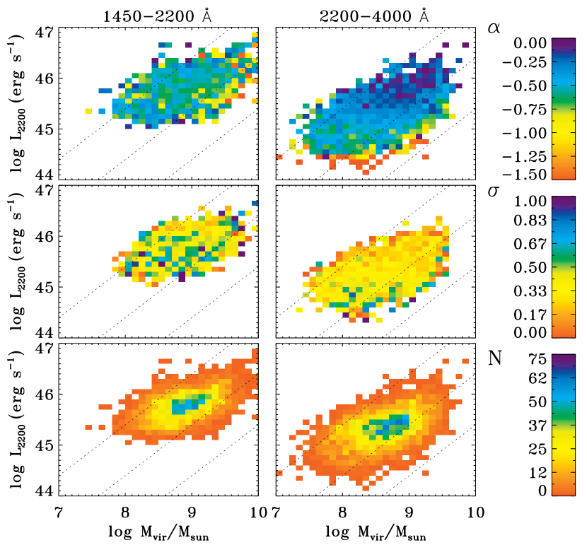
Figure 4.— 2D distributions binned by monochromatic luminosity $L_{2200}$ and the viral mass estimate $M_{\rm vir}$. The left and right panels correspond to the samples with slopes measured from 1450-2200 Å and 2200-4000 Å, respectively. The top panels display the mean slopes $\alpha$, the middle panels show the standard deviation of $\alpha$ in each bin, and the bottom panels represent the number of spectra contributing to each bin. The diagonal dotted lines are approximate estimates for curves of constant Eddington ratio, assuming $L_{\rm bol}=5L_{2200}$. See the text in §4.2 for further disscussion.

The distributions of $\alpha$ for the two samples are plotted in Figure 2. The mean slopes for the two samples are -0.59 from 1450-2200 Å (thin curve) and -0.37 from 2200-4000 Å (thick curve). The differences in the distribution of $\alpha$ between the two samples suggests that the QSO spectra may be slightly concave with redder slopes at shorter wavelengths. This observation is consistent with the slope measurement for the relatively nearby AGN summarized in Table 1, which are always redder at shorter wavelengths.

In Figure 3 we plot the mean slope $\alpha$, binned in terms of $M_{\rm vir}$ and $L_{2200}\equiv\lambda L_{\lambda}$ evaluated at 2200 Å. The error bars represent uncertainty estimates for $\alpha$, corresponding to $\sigma/\sqrt{N}$, where $N$ is the number of spectra which contribute to the bin and $\sigma^{2}=\sum(\alpha-\bar{\alpha})^{2}/(N-1)$ is the variance in each bin. Differences in the distributions of $\alpha$ between the two samples are clearly evident. The higher redshift, shorter wavelength sample shows weak anticorrelations of $\alpha$ with $L_{2200}$ and $M_{\rm vir}$. In contrast, the lower redshift, longer wavelength sample suggests that $\alpha$ is positively correlated with both $L_{2200}$ and $M_{\rm vir}$. The strongest trend is the nearly monotonic rise in $\alpha$ as $L_{2200}$ increases. There also appears to be a weaker trend in which $\alpha$ increases as $M_{\rm vir}$ increases to $\sim 10^{9}M_{\odot}$, but then turns over and begins to decreases at higher masses.

In order to examine possible correlations between the parameters, we plot a 2D distribution of $\alpha$ in the top panel of Figure 4. We bin the data in both $L_{2200}$ and $M_{\rm vir}$ simultaneously. In this plot and several to follow, the left and right hand columns correspond to quantities measured using the 1450-2200 Å and 2200-4000 Å samples, respectively. In the middle panel we plot the standard deviation $\sigma$, and in the bottom panel we plot $N$. The diagonal dashed lines provide a simple, although relatively crude, estimate of the Eddington ratio. They are curves of constant $L_{2200}/M_{\rm vir}$ and would correspond to lines of constant Eddington ratio if a linear relationship between bolometric luminosity $L_{\rm bol}$ and $L_{2200}$ held for all sources. From right-to-left each curve represents a factor of 10 increase in this ratio and the left-most line would correspond to the Eddington limit. For this estimate, we assume a ratio $L_{\rm bol}/L_{2200}=5$, but do not regard this exact value as particularly significant. Since the mean ratio of $L_{2200}/L_{3000}\sim 6/5$ in our sample, this choice provides approximate consistency with the $L_{\rm bol}/L_{3000}=5.9$ relation estimated by McLure & Dunlop (2004).

We find that the 1450-2200 Å slopes are not strongly correlated with either $L_{2200}$ or $M_{\rm vir}$. The highest concentration of blue slopes are found at low $L_{2200}$ and low $M_{\rm vir}$ while the highest concentration of red slopes occurs at low to moderate $L_{2200}$ and high $M_{\rm vir}$ (i.e. low $L/L_{\rm Edd}$). There is a clear trend in the 2200-4000 Å slopes in which $\alpha$ decreases as $L_{2200}$ decreases at fixed $M_{\rm vir}$. A weaker variation with $M_{\rm vir}$ can also be inferred, even at fixed luminosity, although it is strongest at high and low $M_{\rm vir}$ where $N$ tends to be lower. At fixed $L_{2200}$, $\alpha$ first increases with increasing $M_{\rm vir}$ and then decrease at high $M_{\rm vir}$ and low $L/L_{\rm Edd}$, consistent with Figure 3. Comparison of $\sigma$ and $\alpha$ in the top two panels shows that the typical variance in each bin can be quite large relative to the observed trends. The strongest trend in the data, the variation in $\alpha$ from $L_{2200}\sim 5\times 10^{44}-10^{46}$ erg s^-1 at long wavelengths, corresponds to $\Delta\alpha\sim 0.45$ while $\sigma\gtrsim 0.3$ is common. We attribute some, but not all, of this scatter to errors in the flux measurements, for which $\sigma_{\alpha}\lesssim 0.15$ is typical.

Obviously, the variation of $\alpha$ with monochromatic luminosity depends to some extent on the wavelength used to evaluate it. Since it is the ratio of $L_{2200}$ to $L_{4000}$ determines $\alpha$ in the first place, a positive (negative) correlation between $\alpha$ and $L_{2200}$ ($L_{4000}$) would occur if the logarithmic ratio of these luminosities were randomly distributed about some mean ratio. We plot the distribution of $\alpha$, binned by $L_{4000}$ in Figure 5. As might be expected, we find a weaker, but still positive, correlation between $\alpha$ and $L_{4000}$ than we found between $\alpha$ and $L_{2200}$ (cf. Figure 3).

Figure 5.— 1D distribution of mean slopes $\alpha$ binned by monochromatic luminosity at 4000 Å. The slopes are measured from 2200-4000 Å. Error bars are calculated assuming uncertainties $\sigma/\sqrt{N}$ where $\sigma$ and $N$ are the standard deviation and number of spectra in each bin.

5. Model Slopes and Monte Carlo Comparisons

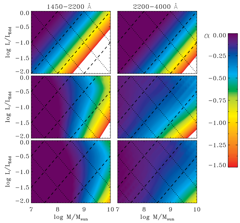
Figure 6.— Slopes calculated from artificial SEDs of relativistic thin disk models (Hubeny et al., 2000). The left and right panels correspond to the slopes measured from 1450-2200 Å and 2200-4000 Å, respectively. In the upper and middle panels we plot spectra from relativistic models of accretion onto a Schwarzschild black hole. The bottom panels show slopes calculated for a black hole with $a_{\ast}=0.9$. For the spectra in the top panels, we approximate the emission at the disk surface as blackbody with the local effective temperature. In the middle and bottom panels, the emission is based on non-LTE spectral atmosphere calculations. The diagonal dashed lines correspond to lines of constant $T_{\rm in}$ and the diagonal dotted lines represent lines of constant $L$. See the text in §5.1 for further discussion.

5.1. Model Slopes

We now wish to more carefully examine the model SEDs described in §2. Although the models we use are rather sophisticated in how they treat radiative transfer and disk structure, it is useful to begin by considering a simple case. Perhaps the simplest spectral model one can construct is the multitemperature blackbody. In this case one simply calculates the radiative flux in the disk as a function of radius and computes a spectrum by integrating the emission over the disk surface, assuming a Planck spectrum $B_{\nu}$ at the local effective temperature $T_{\rm eff}$. This yields

$$L_{\nu}=4\pi^{2}\int B_{\nu}(T_{\rm eff}(R))RdR.$$ (3)

To proceed further, one must obtain $T_{\rm eff}$ as a function of $R$. A common approximation is to assume a power law form for the flux $F\propto R^{-\beta}$, yielding

$$T_{\rm eff}=T_{\rm in}\left(\frac{R}{R_{\rm in}}\right)^{-\beta/4}.$$ (4)

Inserting this form into equation (3) yields

$$L_{\nu}=\frac{240R_{\rm in}^{2}\sigma T_{\rm in}^{3}h}{\pi^{3}k_{\rm B}\beta}\left(\frac{h\nu}{k_{\rm B}T_{\rm in}}\right)^{3-8/\beta}\int_{x_{\rm in}}^{x_{\rm out}}\frac{x^{8/\beta-1}}{e^{x}-1}dx,$$ (5)

where $x\equiv h\nu/(k_{\rm B}T)$. Note that in addition to the explicitly power law dependence on $\nu$, $L_{\nu}$ is also a function of $\nu$ through the limits of the integral $x_{\rm in}=h\nu/(k_{\rm B}T_{\rm in})$ and $x_{\rm out}=h\nu/(k_{\rm B}T_{\rm out})$, For $h\nu\ll k_{\rm B}T_{\rm out}$ and $h\nu\gg k_{\rm B}T_{\rm in}$ we have $L_{\nu}\propto\nu^{2}$ and $L_{\nu}\propto\nu^{3}\exp{(-h\nu/k_{\rm B}T_{\rm in})}$, respectively. At intermediate frequencies $k_{\rm B}T_{\rm in}\gg h\nu\gg k_{\rm B}T_{\rm out}$, the integral is almost independent of $\nu$ and we find $L_{\nu}\propto\nu^{3-8/\beta}$, or $\alpha=3-8/\beta$.

For a Newtonian thin disk the flux is given by (Shakura & Sunyaev, 1973)

$$F=\frac{3GM\dot{M}}{8\pi R^{3}}\mathcal{I},$$ (6)

where $R$ is the radius and $\mathcal{I}$ is a correction factor which depends on assumptions about the torque at the inner edge of the disk. Typically, $\mathcal{I}$ is only a weak function of $R$ which approaches unity at large $R$, so we will ignore it for this simple example. Then $\beta\simeq 3$ and $\alpha\simeq 1/3$ well below the peak in the SED.

For a black hole of mass $M$, it is useful to scale $R$ with $R_{g}\equiv GM/c^{2}$ and $\dot{M}$ with $\dot{M}_{\rm Edd}\equiv L_{\rm Edd}/c^{2}=4\pi GM/(c\kappa_{\rm es})$, where $\kappa_{\rm es}$ is the electron scattering opacity. With the scalings $\dot{m}\equiv\dot{M}/\dot{M}_{\rm Edd}$ and $r=R/R_{g}$, we find

$$T_{\rm in}=\left(\frac{3c^{5}\dot{m}}{2\sigma GM\kappa_{\rm es}r_{\rm in}^{3}}\right)^{1/4}.$$ (7)

These results suggest that $\alpha\sim 1/3$ for $h\nu\ll k_{\rm B}T_{\rm in}$, with $T_{\rm in}$ given by equation (7). This result, first derived by Lynden-Bell (1969), is commonly referenced as a characteristic spectral slope for accretion disks (Frank et al., 1992), but we shall see below that more sophisticated models generically give lower values of $\alpha$ for the masses and luminosities considered in this work. In part, this will be due to the breakdown of the underlying assumptions: that the emission is blackbody and that the flux is given by a simple power law with $\beta=3$. However, it will also not always be the case that $h\nu\ll k_{\rm B}T_{\rm in}$ at the UV wavelengths we are considering. As $M$ increases or $\dot{m}$ decreases, the frequency at which the SED peaks ($\nu\sim 3k_{\rm B}T_{\rm in}/h$) decreases. For $h\nu\lesssim k_{\rm B}T_{\rm in}$, the spectrum should begin to flatten and $\alpha$ is expected to decrease.

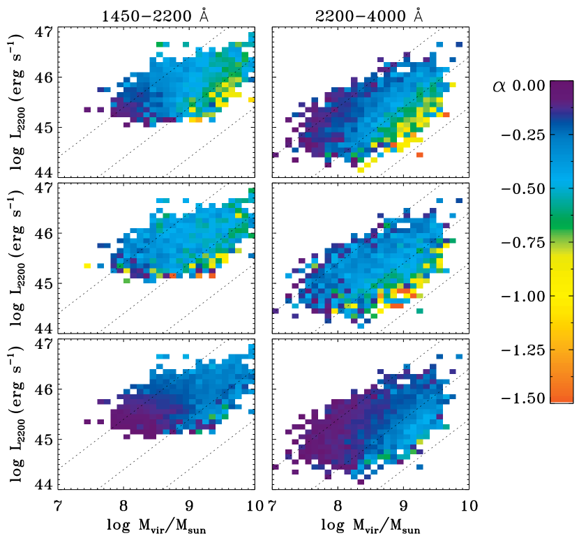
Figure 7.— Simulated 2D distributions of $\alpha$ binned by $L_{2200}$ and $M_{\rm vir}$ for comparison with the top panels of Figure 4. The left and right panels correspond to the slopes measured from 1450-2200 Å and 2200-4000 Å, respectively. The distributions of $\alpha$ are calculated from thin disk models using a Monte Carlo method described in §5.2 to approximate the distribution of mass and luminosity. Each row corresponds to a different set of assumptions for the black hole spin and the uncertainties in the mass estimates. In the top and middle panels we plot $\alpha$ calculated for models with $a_{\ast}=0$ while the bottom panels show the results for $a_{\ast}=0.9$. The top and bottom panels assume $\sigma_{M}=0.4$ dex, while the middle panels assume $\sigma_{M}=0.8$ dex.

This trend is clearly seen in Figure 6, where we have calculated $\alpha$ from 1450-2200 Å and 2200-4000 Å, using equation (2). In the top panel, we compute $\alpha$ for relativistic, multitemperature models with $a_{\ast}=0$. We plot $\alpha$ as a function $L/L_{\rm Edd}$ ($\propto\dot{m}$), where $L$ is the model bolometric luminosity. The shape of the spectrum, and therefore, $\alpha$ depends (weakly) on inclination. Here we plot the mean $\alpha$, averaged over a uniform distribution in $\cos i$ from $\cos i=0.5$ to 1. The diagonal dashed and dotted curves correspond to lines of constant $T_{\rm in}$ and constant $L$, respectively. $L$ increases from bottom left to top right and $T_{\rm in}$ increases from the top left to bottom right. In this case, $\alpha$ can be entirely parameterized by $T_{\rm in}$. Since the 1450-2200 Å slopes are measured with continuum windows nearer to the peak in the SED, it is always the case that $\alpha$ is lower than measurements made from 2200-4000 Å. We note that even for these blackbody models, $\alpha$ is less than the “canonical” value of 1/3 over the entire parameter space of interest.

In the middle panels of Figure 6 we again plot $\alpha$ for $a_{\ast}=0$ models, but with spectra based on the atmosphere models described in §2. For 2200-4000 Å slopes, we again find that the variations in $\alpha$ can largely parameterized by $T_{\rm in}$, although not completely. The primary difference is that the slopes are lower than the multitemperature blackbody models and the overall variation with $T_{\rm in}$ tends to be weaker. There are several effects which may contribute to these differences, but at these wavelengths the most important modification to the spectrum is the Balmer edge at 3650 Å. For the majority of annuli which contribute to the emission near 4000 Å, there is a strong Balmer edge in absorption. The flux emitted by any annulus is fixed by the local dissipation of energy, so the decrement in flux shortward of the edge is compensated by an increase longward of the edge. At 2200 Å the effects of the Balmer edge are minimal. The net effect is to increase the ratio 4000 Å to 2200 Å flux relative to what it would be if the edge was absent, yielding a lower $\alpha$.

The differences in the 1450-2200 Å slopes between the two models are greater. The contours of constant $\alpha$ are generally more vertical. At high $M$ and $L/L_{\rm Edd}$, they actually turn over and nearly follow the lines of constant $L$ (dotted curves). Compared with the multitemperature blackbody models, we find that $\alpha$ is generally higher, particularly at low $L$, and only at high $L$ is $\alpha$ lower than the blackbody prediction.

The differences between the model slopes at shorter wavelengths are largely due to the increasing importance of electron scattering opacity in annuli where these photons are primarily emitted. As the ratio of scattering to absorption opacity increases the spectrum of a particular annulus becomes a “modified blackbody” (see e.g. Rybicki & Lightman, 1979) which peaks at higher photon energies. Since total flux is conserved, the increase in higher energy photons must be offset by a decrease in the flux at lower energies. The emission at any particular wavelength $\lambda$ (in this case 1450 Å) is going to come from a range of annuli with $T_{\rm eff}\sim ch/(3k_{\rm B}\lambda)$. When compared with blackbody emission, some of these annuli will contribute more flux to $\lambda$ and some will contribute less. The net effect when emission is integrated over all annuli will depend on a number of factors: how close $T_{\rm eff}$ is to $T_{\rm in}$, the wavelength at which $\kappa_{\rm es}$ becomes the dominant opacity, and how strongly the spectrum is deformed from blackbody. For low values of $T_{\rm in}$ and low $L$ this deformation tends to enhance the flux at 1450 Å, but has little effect on the flux at 2200 Å, increasing $\alpha$.

In the bottom panels, we again plot slopes for atmosphere based spectra, but with $a_{\ast}=0.9$ instead of $a_{\ast}=0$. The dependence of $\alpha$ on $L/L_{\rm Edd}$ and $M$ is very similar to the $a_{\ast}=0$ case in that contours of constant $\alpha$ have similar shapes. However, the spectra are generically bluer since $\alpha$ is larger than the $a_{\ast}=0$ slopes over the whole range covered by the plot. There are multiple ways in which changing $a_{\ast}$ modifies $\alpha$, but the dominant effect is the shift in the peak of the SED. In these models, the inner radius $r_{\rm in}$ is determined by the location of the innermost stable circular orbit (ISCO), which is smaller for larger $a_{\ast}$. From equation (7), we can see that this makes $T_{\rm in}$ larger. At fixed $L/L_{\rm Edd}$, $\dot{m}$ must also decrease to offset the increase in radiative efficiency, which would reduce $T_{\rm in}$. However, the former effect dominates, and the peak of the SED shifts to shorter wavelengths, generally increasing $\alpha$.

5.2. Monte Carlo Comparisons

With accurate mass, spin, and inclination estimates, we could compare the slopes in Figure 4 directly with the models, such as those shown in Figure 6. However, we do not have any practical means of estimating either the spin or the inclination. Furthermore, we do not know with certainty the accuracy of mass estimates $M_{\rm vir}$ obtained with equation (1). In order to account for these uncertainties we construct slope distributions similar to those shown in Figure 4 using Monte Carlo methods.

In order to characterize the distributions of model parameters we must make several assumptions. First we must adopt a distribution of inclinations. In absence of obscuration, a uniform distribution in $\cos i$ would be expected from isotropic emission. However, the disk models do not produce isotropic emission. Disks viewed nearly face on ($\cos i\sim 1$) have larger fluxes than edge-on disks, and should be somewhat enhanced near the flux limit in a flux limited sample. Furthermore, angle dependent obscuration is a fundamental tenet of the unified model of AGN (Antonucci, 1993). In the unified model, obscuring material lies in the disk plane (the “torus”). Broad emission line objects, such as the type I QSOs discussed here, will be viewed nearly face on, up to the opening angle of the torus. Here, we adopt a uniform distribution in $\cos i$ from $\cos i=0.5$ to 1, where the lower limit corresponds to an opening angle of $60^{\circ}$. Since the differences in $\cos i$ produce at most a factor of two in flux, the assumption of a uniform distribution will only produce a small error near the flux limit.

We must also specify $a_{\ast}$. Unfortunately the distribution of $a_{\ast}$ is highly uncertain. Estimates for $a_{\ast}$ in AGN are limited to a handful of bright, relatively nearby sources with broad Fe K$\alpha$ lines. In some cases, such as MCG -6-30-15, very high values of $a_{\ast}$ ($\sim 1$) are inferred (see e.g. Tanaka et al., 1995). A combination of empirical and theoretical arguments seem to favor $a_{\ast}\sim 0.9$ (Gammie et al., 2004), although there are considerable uncertainties. Given the large uncertainties, we simply choose two characteristic spins, $a_{\ast}=0$ and 0.9, as representative examples.

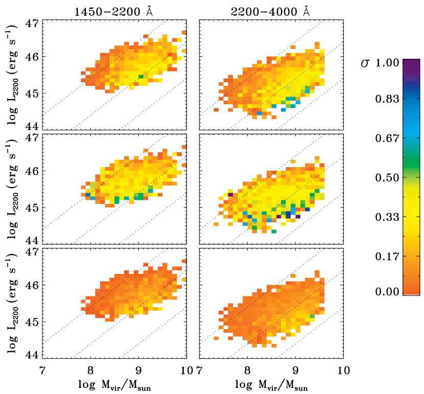
Figure 8.— The standard deviation $\sigma$ for the simulated distributions of $\alpha$ plotted in Figure 7. Each row correspond to a different set of assumptions for the black hole spin and the uncertainties in the mass estimates, as described in the caption of Figure 7.

Finally, we must account for the uncertainties in $M_{\rm vir}$. Although these uncertainties are difficult to estimate robustly, some insight may be obtained by comparing estimates which utilize the H$\beta$ line width and monochromatic luminosity at 5100 Å. McLure & Dunlop (2004) compute the ratio $\log(M_{\rm vir}[{\rm H}\beta]/M_{\rm vir}[{\rm Mg~{}II}])$, finding a dispersion of 0.33 dex. This, of course, does not account for any systematic errors common to the two methods. The $M_{\rm vir}[{\rm H}\beta]$ estimates rely on luminosity based $R_{\rm BLR}$ estimates which are calibrated by matching reverberation mapping estimates. For example, Vestergaard (2002) find that 70% of $M_{\rm vir}[{\rm H}\beta]$ mass estimates match the reverberation mapping estimates to within a factor of 3. The reverberation mapping estimates, in turn, are claimed to have a typical precision of $\sim 30\%$ (Peterson et al., 2004). Here, we adopt 0.4 dex as a fiducial value of the uncertainty in $\log M_{\rm vir}$. Given the scatter in the relations discussed above, we view this as a lower limit on the typical error. Therefore, we also consider the impact of assuming a larger uncertainty (0.8 dex) below.

With these assumptions we can begin computing Monte Carlo slope distributions. We start by assuming a distributions of $L_{2200}$, $v_{\rm Mg}$, and $M_{\rm vir}$ identical to those in §4.2. Next, we use random deviates to draw values of the “actual mass” $M_{0}$ and $\cos i$. Here, $M_{0}$ is used to account for possible errors in the mass estimates. It is drawn from a log normal distribution with a mean of $M_{\rm vir}$ and $\sigma_{M}=0.4$ dex. This prescription means that the mass distribution of the models will be somewhat broader than the distribution of $M_{\rm vir}$. However, there is some evidence for a real cutoff in the mass distribution at high mass. Therefore, we enforce a maximum mass $\log M_{0}/M_{\odot}<9.5$. Then, for each choice of $M_{0}$ and $i$, a value of $L/L_{\rm Edd}$ is chosen so the model monochromatic luminosity matches $L_{2200}$. Finally, given these values of $L/L_{\rm Edd}$, $M_{0}$, $i$, and a choice of $a_{\ast}$ we can compute $\alpha$ for the corresponding model. These slopes are then binned in exactly the same manner as the data, allowing us to compare with the observed $\alpha$ and $\sigma$. (Note that the distributions of $N$ are identical to the observations by construction.)

We plot the resulting 2-D distribution of $\alpha$ for $a_{\ast}=0$ in the top panels of Figure 7. For both long and short wavelength slopes, there are clear mass and luminosity dependent trends in $\alpha$. At fixed $L_{2200}$, $\alpha$ decreases with increasing $M_{\rm vir}$ and at fixed $M_{\rm vir}$, $\alpha$ generally decreases with decreasing $L_{2200}$. Since $L_{2200}$ is roughly proportional to the bolometric luminosity, the trends are as expected from middle left panel of Figure 6. Comparison with Figure 4 shows that these strong variations are clearly discrepant with the weak trends in $\alpha$ inferred from the observations. Although we do not plot the results, we have performed the equivalent exercise using the multitemperature blackbody slopes. The model trends are even stronger, due the rapid reddening of the spectra at high masses and low luminosities. The discrepancies are particularly large at short wavelengths, where the multitemperature blackbody slopes are significantly redder than the observed spectra.

In the the top panel of Figure 8, we plot the distribution of standard deviations corresponding to the slopes in Figure 7. The distributions of $\sigma$ are largely determined by the assumed uncertainty in $M_{\rm vir}$ . If the assumed uncertainty $\sigma_{\rm M}$ was identically zero, each $\alpha$ would be almost completely determined by $L_{2200}$ and $M_{\rm vir}$ since the variation in $\alpha$ with $\cos i$ is relatively weak. In that case, $\sigma\lesssim 0.05$ would be typical. However, comparison with the middle panel of Figure 4 shows that despite this scatter induced by the mass uncertainties, $\sigma$ for the model slopes is still substantially below the standard deviations obtained from the observed slopes.

Given the nature of the discrepancy between models and data, an obvious concern is the effect of errors in the mass estimates. If the errors in the mass estimates are larger, they might smear out any mass dependence in the observed slopes and increase $\sigma$. Of course, the actual form of the mass error distribution remains an important source of uncertainty, and the log normal distribution employed here may not be an adequate approximation. However, since we have no reliable means of independently measuring this distribution, we simply accept this as a caveat and consider the effects of larger errors by increasing $\sigma_{M}$ from 0.4 to 0.8 dex. We plot the results in the middle panels of Figures 7 and 8.

In the middle panel of Figure 7, we find that the resulting distributions of $\alpha$ are still incapable of reproducing the observations, but increasing $\sigma_{M}$ to 0.8 dex does smear out the strong variation seen the $\sigma_{M}=0.4$ dex case, as expected. At short wavelengths, this removes almost all of the variation in the slopes with $M_{\rm vir}$ and $L_{2000}$, in better agreement with the lack of a strong trend in the observed slopes. However, the mean slopes are still larger than those that are observed. At longer wavelengths, there is still some trend for larger slopes for higher $L/L_{\rm Edd}$, which is inconsistent with the observed distribution. For $L/L_{\rm Edd}\gtrsim 0.1$, the model slopes are too large at low $L_{2000}$ and too low at high $L_{2000}$.

In the middle panels of Figure 8, we find that $\sigma$ also increases, as expected. This provides better agreement with observed $\sigma$, although $\sigma$ is still generally too low. We also find that $\sigma$ decreases as $L/L_{\rm Edd}$ increases, a trend not seen in the data. This decrease in $\sigma$ is also consistent with Figure 6, which shows that $\alpha$ is a weaker function of $L/L_{\rm Edd}$ and $M$ for the low $M$ and high $L/L_{\rm Edd}$ models which predominantly contribute to the low $\sigma$ bins.

Except at high luminosities and long wavelengths, we nearly always find that the models predict $\alpha$ larger (bluer) than the observed values. A comparison of the bottom and middle panels of Figure 6 suggests that increasing $a_{\ast}$ will only make the discrepancy worse, since the $a_{\ast}=0.9$ models slopes are everywhere larger than the $a_{\ast}=0$ case at equivalent $M$ and $L/L_{\rm Edd}$. Indeed, this is precisely what we find in the bottom panels of Figures 7 when we plot $\alpha$ for $a_{\ast}=0.9$ and $\sigma_{M}=0.4$ dex. For the range of $M_{\rm vir}$ and $L_{2000}$ sampled, $\alpha$ varies less strongly than in the $a_{\ast}=0$ case. However, this also means that $\sigma$ is even lower, increasing the disagreement with the data. Thus, it appears that the $a_{\ast}=0.9$ models are an even poorer match to the data that the $a_{\ast}=0$ models. This result may be problematic since, as discussed above, there is some evidence which suggests $a_{\ast}\gtrsim 0.9$ may be more common than $a_{\ast}\sim 0$.

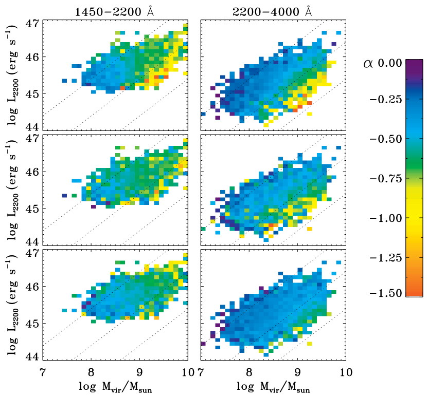
Figure 9.— Simulated 2D distribution of $\alpha$ binned by $L_{2200}$ and $M_{\rm vir}$.The left and right panels correspond to the slopes measured ¿ from 1450-2200 Å and 2200-4000 Å, respectively. The distributions account for the effects of dust extinction with an SMC-like reddening curve (see text), but are otherwise equivalent to those plotted in Figure 7. We calculated each distribution assuming a uniform distribution in E(B-V) between 0 and a specified maximum value chosen to match the observed short wavelength slopes of Figure 4. We assume a maximum $\rm E(B-V)=0.03$ for the $a_{\ast}=0$ models (top and middle panels), and $\rm E(B-V)=0.03$ for the $a_{\ast}=0.9$ models (bottom panels).

6. Discussion and Conclusions

6.1. The Effects of Dust Reddening on Spectral Slopes

It is clear that some additional process (or processes) must be modifying the spectrum if the models are to be reconciled with the observed slopes and we discus a number of possibilities below. One of the main discrepancies is that the observed spectra are generally redder than the models predict. One likely possibility is that the SEDs are altered by wavelength dependent extinction from dust intrinsic to the source or host galaxy. Dust emission can be seen in the infrared in many AGNs, and is almost certainly present at some level in our sample (see e.g. Richards et al., 2003). The uncertainties are mainly questions of how much dust is present and what is the wavelength dependence of the extinction.

We can incorporate the effects of dust reddening directly into our Monte Carlo distributions by simulating the effect of extinction on the model SEDs. Multiplying our artificial spectra by a reddening curve will change both the values of $\alpha$ and $L_{2200}$ inferred by an observer. In order to proceed we must specify the shape of the reddening curve and specify the amount of extinction. Often, the degree of reddening is parameterized by the color excess E(B-V) which is the difference in extinction between the B and V bands, expressed in magnitudes. Since this distribution is unknown, we simply adopt a uniform distribution of color excess between zero and some specified maximum value.

The wavelength dependence of the extinction is also uncertain. The determination of QSO reddening curves is an area of active research and ongoing debate (Richards et al., 2003; Gaskell et al., 2004; Hopkins et al., 2004; Czerny et al., 2004; Willott, 2005). Much of the difficulty in determining these reddening curves stems from the problem of disentangling intrinsic variations in the quasar SED (lines or continuum) from the effects of dust. This makes it difficult to unambiguously identify “unreddened” AGN sources for comparison with a “reddened” population. Despite this uncertainty, it is widely accepted that the $\sim 2200$ Å feature seen in the Galactic interstellar medium (see e.g. Cardelli et al., 1989) is extremely weak or absent in AGN reddening curves.

Disagreement primarily arises over the steepness of the reddening curve, particularly at wavelengths shortward of $\sim 3000$ Å. For example, Gaskell et al. (2004) derive a flat far UV reddening curve, while the analysis of Hopkins et al. (2004) favors a steeper, SMC-like curve. Another calculation by Czerny et al. (2004), which is based on ratios of the color selected SDSS quasar composites of Richards et al. (2003), prefers a curve which is in between: somewhat flatter than the SMC, but still steeper than that found by Gaskell et al. (2004).

Clearly, if extinction is important, the observed slope distributions will depend significantly on the form of the reddening curve. Therefore, we have considered three possibilities: the approximate forms of the curves derived by Gaskell et al. (2004) (see their Appendix) and Czerny et al. (2004) (equation [3]), and the SMC-like curve used by Richards et al. (2003) ($A_{\lambda}=1.39\;E(B-V)(\lambda/\mu{\rm m})^{-1.2}$).

In Figure 9 we plot Monte Carlo distributions equivalent to those in Figure 7, but including the effects of dust. For this example we use the SMC-like reddening curve and choose maximum E(B-V) so that short wavelength slopes approximately match the observed slopes (cf. Figure 4). This matching requires E(B-V) $\sim 0.03$ and $0.055$ for $a_{\ast}=0$ and 0.9, respectively. These modest values would not contradict the results of Richards et al. (2003) who found that 94% of their sample would be consistent with E(B-V) $<0.04$ for the same reddening curve. We note that the modification of $L_{2200}$ due to extinction is typically small for the required range of E(B-V). In principle, a larger amount of extinction could introduce a correlation where dust reddened sources are less luminous than bluer, unreddened spectra, and possibly explain the observed trend of higher $\alpha$ for higher $L_{2200}$. Also, the small amount of extinction at 2200 Å introduces considerably less scatter in $\alpha$ than the uncertainties in the mass estimate. Therefore, we do not replot the standard deviation of the bins, since the plots differ little from those of Figure 8.

The reddening curve of Czerny et al. (2004) has a flatter wavelength dependence than the SMC-like curve, and therefore requires greater extinction to produce the same amount of reddening. In order to match the short wavelengths slopes of Figure 4, we require a maximum E(B-V) $\sim 0.6$ and 0.12 for $a_{\ast}=0$ and 0.9, respectively. The relative flatness of this reddening curve in comparison to the SMC-like curve also leads to a greater degree reddening at longer wavelengths to produce the same amount of reddening a short wavelengths. This is particularly significant for $a_{\ast}=0.9$ model. Since the observed slopes are redder at lower $L_{2200}$, this improves the agreement with the data for low $L_{2200}$, but provides a poorer match for higher values of $L_{2200}$, where slopes are bluer.

The Gaskell et al. (2004) curve is nearly flat shortward of 3000 Å. Therefore, it requires substantially greater extinction to compensate for the slope discrepancy between the models and data at short wavelengths. We cannot easily parameterize the amount of extinction required because it is large enough to boost the intrinsic (unreddened) luminosity by an order of magnitude or more. This would make the models substantially super-Eddington for the assumed masses, exceeding the upper limit of our grid where the thin disk assumptions are no longer self-consistent.

Although our assumed distribution of color excess which is uncorrelated with luminosity can improve the agreement between the models and data at short wavelengths, it cannot reproduce the $L_{2200}$ dependent trend at longer wavelengths. To some degree, this conclusion hinges on our assumption that the amount of dust extinction is independent of luminosity. If, for example, the amount of dust extinction anticorrelates with luminosity, the most luminous QSOs could have unreddened, intrinsically blue spectra while lower luminosity QSOs would have lower slopes due to the dust reddening, in agreement with the observed trend. However, the lack of a similar luminosity dependent correlation at short wavelengths would then require a reddening curve which is flat shortward of $\sim 2200$ Å, such as that proposed by Gaskell et al. (2004). Since the short wavelength slopes are redder than predicted by the models, matching the data with the models at short wavelengths is not possible with such a flat reddening curve. Therefore, even if such luminosity dependent redding is plausible, it seems unable to simultaneously account for both the short and long wavelength spectral slopes if the underlying continuum is well approximated by the models. However, such a scenario may account for the observed trend if the short wavelength continuum is intrinsically redder than the models predict.

6.2. The Effects of Irradiation

Self-irradiation presents another possibility for explaining the red slopes in these systems. In fact, correlated variability on timescales comparable to the light travel times suggests that irradiation must be occurring at some level (see e.g. Krolik et al., 1991). In the UV, we expect irradiation to become increasingly less important for determining the spectrum as we move to shorter wavelengths in the UV, since local dissipation must dominate the flux near the peak of the SED. Nevertheless, irradiation may still play some role so we briefly consider its effects by examining a simple model.

The slope modification due to reddening will be strongly dependent on the geometry of the accretion flow. A simple estimate of the slopes of irradiated disks may be obtained from equation (5) which implies $\alpha=3-8/\beta$ for $h\nu\ll k_{\rm B}T_{\rm in}$. In order to estimate $\beta$, we need to specify the radial dependence of the irradiated flux $F_{\rm irr}\propto R^{-\beta}$. With simple geometric arguments, one can show (see e.g. Blaes, 2004b) that

$$F_{\rm irr}=\frac{L_{\ast}(1-a)}{4\pi R^{2}}\left(\frac{H}{R}\right)\left(\frac{d\log H}{d\log R}-1+\frac{H_{\ast}}{R}\right).$$ (8)

In order to obtain this relation, we approximate the irradiating continuum (the inner disk, or possibly a corona) as a point source $L_{\ast}$ at $R=0$ and a height $H_{\ast}$ above the midplane. The disk surface at the point of irradiation is parameterized by the height $H(R)$ at radius $R$. The albedo $a$ may also be a function of $R$, but we will ignore this dependence for simplicity.

For $H_{\ast}\gg H(R)$, we find $F_{\rm irr}\propto R^{-3}$. This dependence is easily understood by noting that emission from the point source falls off as $R^{-2}$ and is intercepts the disk surface with angle $\theta$ such that $\cos\theta=H_{\ast}/R$. Since $H_{\ast}$ is independent of $R$, we find $F_{\rm irr}\propto R^{-3}$ as inferred from equation (8). If this reprocessed flux dominates the locally dissipated flux and is reradiated as a blackbody we again have $\beta=3$ and $\alpha=1/3$, equivalent to the bare thin disk case.

If $H_{\ast}\leq H(R)$, the disk must flare in order to produce significant irradiation. If we parameterize $H$ as a power law ($H\propto R^{\Gamma}$), we find $\beta=3-\Gamma$ or $\alpha=(1-3\Gamma)/(3-\Gamma)$. An important case is $\Gamma=1$ for which $\beta=2$ and $\alpha=-1$. For $\Gamma>1$, $\alpha<-1$ and vice-versa. This suggests that in the region of parameter space where most of our slopes lie, $-1<\alpha<1/3$, we require $\Gamma<1$. Such models are concave in shape and self-shielding at sufficiently large radii.

Obtaining slopes in this range via irradiation may therefore require some level of fine tuning. One possibility is that the disk transitions from a flat or convex ($\Gamma>1$) solution to a concave ($\Gamma<1$) solution at the range of radii which give rise to the UV emission so that self-shielding occurs only at larger radii and longer wavelengths. A second possibility is that there is flaring with $\Gamma>1$, but that the reprocessed flux does not dominate the local dissipation. The differing fraction and radial dependences of the local dissipation and reprocessed flux give rise to a range of $\alpha$ between $\sim-1$ and $\sim 1/3$. Such a concurrence would be somewhat surprising, because a comparable contribution from the locally dissipated and reprocessed emission will only occur over a limited range of radii, due to their different radial dependences.

Nevertheless, self-shielding geometries may be useful for explaining some aspects of the observed slope distribution. In the top panel of Figure 4 we see that for the highest luminosity sources, slopes are, on average, bluer at longer wavelengths than at short wavelengths. The redder than expected slopes at short wavelengths could be produced by irradiation of a portion of the disk surface which blocks emission from reaching larger radii. The unirradiated flow at larger radii and lower $T_{\rm eff}$ could remain dominated by the local dissipative flux and produce an intrinsically bluer slope.

In order for such interpretations to be valid, the geometry of the irradiated accretion flows needs to be explained. Our thin disk models for supermassive black holes are radiation pressure dominated in their inner-most radii (Shakura & Sunyaev, 1973), implying a scale height which is nearly independent of radius. With this model, we would not expect reprocessing to significantly alter the spectrum until the disk transitions to the gas pressure dominated regime where $H\propto R^{21/20}$ (Shakura & Sunyaev, 1973), yielding $\alpha\sim-1$ if reprocessing dominates the local flux. The transition radius from radiation to gas pressure dominance depends on $M$, $\alpha_{\rm SS}$, $\dot{m}$, and $a_{\ast}$, but is generally located at 200-400 $R_{g}$.

Since the bulk of the UV radiation in our models is radiated at radii $\lesssim 200R_{g}$, some other mechanism must be modifying the disk structure in order to explain the red slopes via irradiation. One possibility is that the vertical extent of these disks may be substantially modified due to the magnetic support, as suggested by numerical simulations (see e.g. Turner, 2004; Hirose et al., 2006). However, at present, such calculations remain too uncertain to yield a predictive model for the reprocessing. Another possibility is that backscattered radiation from an outflow might modify the spectrum (e.g. Nikolajuk et al., 2004), but this will depend on the (unknown) outflow geometry, even if such outflows prove to be common.

6.3. The Dependence of Slope on Luminosity

As discussed in §5.2 and §6.1, the luminosity dependent slopes at long wavelengths present a challenge for the Hubeny et al. (2000) models since the discrepancies cannot be simply attributed dust reddening or errors in the mass estimates. As discussed in §6.1, adding an ad-hoc luminosity dependence to the dust extinction might account for the dependence of $\alpha$ on $L_{2200}$ at long wavelengths, but not without creating problems at shorter wavelengths.

Due to the short baselines involved ($\log(4000/2200)=0.26$ and $\log(2200/1450)=0.18$) the slopes can be substantially modified by relatively small changes in flux of a continuum window. Therefore, we consider “contamination” from the host galaxy and/or the BLR emission as a possible solution. In such a scenario, the observed trend would imply either an increasing contribution to flux at 4000 Å as $L_{2200}$ decreases or an increasing contribution to the flux at 2200 Å as $L_{2200}$ increases. Inspection of the bottom, left panel of Figure 3 shows a variation in the mean slope $\Delta\alpha\sim 0.45$ from $L_{2200}<10^{45}\;\rm erg\;s^{-1}$ to $L_{2200}\gtrsim 10^{46}\;\rm erg\;s^{-1}$. This is only slightly greater than the typical standard deviation in the individual bins and corresponds to a $\sim 30\%$ variation in the relative flux between the two continuum windows.

One scenario would be a contribution from the host galaxy which is roughly independent of the QSO luminosity and contributes $\sim 30\%$ at low $L_{2200}$. Based upon the strength of absorption lines in their composite spectrum Vanden Berk et al. (2001) estimate a 7%-15% contribution at the location of Ca II $\lambda 3933$ and Na I $\lambda 5896$. Therefore, the trend cannot be explained entirely by host galaxy contamination. A second possibility is excess BLR emission at 2200 Å which correlates with $L_{2200}$. Inspection of the Vanden Berk et al. (2001) composite spectrum indicates emission from high excitation Fe II lines is probably the main contaminant at $\sim 2200$ Å. However, a comparison of composite spectra for QSOs with $L_{2200}$ above and below $3\times 10^{45}\;\rm ergs^{-1}$ does not provide evidence for such a large change in the equivalent width of these lines so we conclude that this explanation is also unlikely.

It is also possible that the underlying accretion flow is thin disk, but that the Hubeny et al. (2000) models have not properly accounted for the emission near $\sim 4000$ Å. The model grid only extends to $T_{\rm eff}=10^{4}\;\rm K$, so the emission for annuli in the disk at larger radius and lower $T_{\rm eff}$ are approximated by blackbodies. For models with $T_{\rm eff}\lesssim 10^{4}\;\rm K$ density inversions can occur due to a fall in electron pressure when H recombines (see Fig. 9 of Hubeny et al., 2000). This makes it very difficult to predict the true equilibrium structure, and therefore the spectrum, of an annulus in a real, turbulent accretion flow.

The lack of models $T_{\rm eff}<10^{4}\;\rm K$ creates a problem because these annuli may still have significant Balmer edges. The presence of edge at $\sim 3650$ Å tends to create an excess of emission longward of the edge and a deficit at shorter wavelengths relative to the predictions of a pure blackbody. As can be seen by Figure 11 of Hubeny et al. (2000), replacing non-LTE model spectra with blackbodies may produce a reduction in the flux at 4000 Å. This result, coupled with the observation that the strength of the edge is anticorrelated with luminosity at fixed mass (see Figure 13 of Hubeny et al., 2000), suggests that the Balmer edge may play a greater role in producing the observed trend than the current models predict. A robust determination of the spectrum at these wavelengths might ultimately require spectral models coupled with realistic disk simulations, and is beyond the scope of this work.

It is also possible that selection biases and incompleteness play some role in producing the observed trends. The spectroscopic targeting of QSOs in SDSS is discussed in Richards et al. (2002). For this sample, we consider incompleteness near the flux limit to be the greatest cause for concern since the majority of our sources are well separated from the stellar locus.

The spectroscopic targeting algorithm rejects sources based upon $i$ band magnitude. For $ugri$ and $griz$ selected sources the magnitude limits are $i\lesssim 19.1$ and $i\lesssim 20.2$, respectively. The $i$ band filter is approximately centered at $\sim 7600$ Å, which corresponds to $\sim 3800$ Åand $\sim 2500$ Åfor the low ($z\sim 1$) and high ($z\lesssim 2$) redshift samples respectively. This could lead to a deficit of blue quasars at low $L_{2200}$ in the long wavelength, low redshift sample. For an equivalent $L_{2200}$, red quasars will have a larger flux near 4000 Å than sources with bluer slopes, and would be more likely to make it into the spectroscopic sample if they are near the $i$ flux limit. We have considered this possibility by plotting the slopes as function of $i$ for our sample, but we do not find a significant deficit of blue slopes near the flux limits. In fact, we find a decreasing fraction of red quasars for $i\lesssim 17.5$. This deficit of red spectra with large flux in $i$ seems to be due to a real paucity of red sources with high luminosities.

Figure 10.— Distribution of flux ratios binned as a function of $T_{\rm in}$ for comparison with the results of Bonning et al. (2006). The right and left panels correspond to the slopes measured from 1450-2200 Å and 2200-4000 Å, respectively. We calculate $T_{\rm in}$ from $v_{\rm Mg}$ using the relation $\log T_{\rm in}=5.43-\log(v_{\rm Mg}/3000\;{\rm km\;s^{-1}})$. The top axis displays the value of $\log v_{\rm Mg}$ for comparison with Figure 3. We plot the distribution of the observed SDSS flux ratios as a thin curve. The solid curves show distributions of model flux ratios based on the Monte Carlo distributions. The plotted curves correspond to the same distribution plotted as a 2D distribution in the top panel of Figure 7 with $a_{\ast}=0$ and $\sigma_{M}=0.4$ dex.

6.4. Comparison with Previous Work

There have been a number of previous observational tests of the Hubeny et al. (2000) models considered here. For the most part, these comparisons have involved individual sources or a relatively small sample with broadband spectral coverage. Blaes et al. (2001) fit models to spectra of 3C 273, finding poor agreement in the near UV. The reverberation mapping mass estimate has since been revised, bringing the model and data into better, though not perfect agreement (cf. §3.2).

Blaes (2004a) calculated spectral slopes as a function of mass and Eddington ratio for a subset of sources in the Shang et al. (2005) sample. The results showed significant scatter and rather poor agreement with the model predictions, but the analysis only included a few dozen objects. Using the same data, Shang et al. (2005) compared the optical, optical-to-UV, and far UV spectral slopes to the models, finding rough agreement. A recent analysis of SDSS quasars observed by the Galaxy Evolution Explorer (GALEX) (Trammell et al., 2007) also examined the far UV properties of AGNs, again finding evidence for slope changes near $\sim 1000$ Å, in approximate agreement with the model predictions.

A recent analysis by Bonning et al. (2006) relates most directly to our current work. They use another, overlapping sample of SDSS QSO spectra and measure color ratios between continuum windows located at 1350 Å, 2200 Å, 4000 Å, and 5100 Å. They also compare their results with the a selection of Hubeny et al. (2000) models chosen to approximate the distribution of Eddington ratios and masses inferred from the data.

The choice of variables used for binning is one of the major differences between the Bonning et al. (2006) analysis and this work. Bonning et al. (2006) consider the evolution of observed and artificial spectra as a function of a single variable corresponding to $T_{\rm in}$. For the viral mass estimates used here, the dependence of $T_{\rm in}$ on $v_{\rm Mg}$ and $L_{3000}$ can be obtained by combining equations (1) and (7). If we make the additional assumption that $L_{\rm bol}\propto L_{3000}$, we find

$$T_{\rm in}\propto L_{3000}^{(1-2\delta)/4}v_{\rm Mg}^{-1}.$$

Following McLure & Dunlop (2004), we have used $\delta=0.62$ which yields a weak dependence on luminosity. Bonning et al. (2006) use $\delta=0.5$ exactly so that $T_{\rm in}$ is a function of $v_{\rm Mg}$ alone.

To facilitate comparison, we have replotted our distributions as a function of $T_{\rm in}$ in Figure 10, using flux ratios in place of $\alpha$ on the vertical axis. Following equation (5) of Bonning et al. (2006), we use the relation $\log T_{\rm in}=5.43-\log(v_{\rm Mg}/3000\;{\rm km\;s^{-1}})$ for the horizontal axis. We plot the distributions of both the observed (thin curve) and model (thick curve) flux ratios. The model curves are calculated using the same Monte Carlo distribution as in the top panel of Figure 7. At long wavelengths the observed SEDs are reddest at low and high $T_{\rm in}$. This differs from the model which are red at low $T_{\rm in}$ and become monotonically bluer as $T_{\rm in}$ increases. At short wavelengths the observed flux ratios are roughly independent of $T_{\rm in}$, while the model fluxes are again reddest at low $T_{\rm in}$ and become monotonically bluer as $T_{\rm in}$ increases. These results are qualitatively consistent with Figure 3 of Bonning et al. (2006), who measure colors at 1350 Å as opposed to the 1450 Å window used here.

Bonning et al. (2006) infer that the observed reddening at high $T_{\rm in}$ may be related to Eddington ratio since most of the objects contributing to the highest $T_{\rm in}$ bins have $L/L_{\rm Edd}\gtrsim 0.3$. This is also roughly consistent with our findings. In our sample this result can be understood by examining the top left panel of Figure 4 and considering equation (7). Figure 4 shows that most of the QSOs in our sample do not radiate significantly above the Eddington limit. Equation (7) implies that the highest values of $T_{\rm in}$ are obtained for low values of $M$ and high Eddington ratios (i.e. high $\dot{m}$). As a result, the sources in our sample with the highest $T_{\rm in}$ (and, therefore, low $v_{\rm Mg}$) tend to occupy the low $M_{\rm vir}$, low $L_{2200}$ corner of the plot. Since the observed slopes are predominant functions of $L_{2200}$ with redder slopes at lower luminosities, these QSOs also tend to be redder than average. Of course, bins with slight lower $T_{\rm in}$ also include low $L_{2200}$ objects, but the average $\alpha$ is still larger due to the increasing fraction of higher $M_{\rm vir}$ and $L_{2200}$ sources, which tend to be bluer. Therefore, the problem of understanding the redding at low $T_{\rm in}$ is intimately connected to the question of why the mean slopes are predominantly functions of $L_{2200}$ (rather than $L_{2200}/M_{\rm vir}$) at long wavelengths which we discussed in §6.3:

6.5. Conclusions

We have shown how slopes from artificial SEDs of thin accretion disks (Hubeny et al., 2000) vary with black hole mass and bolometric disk luminosity. As expected from naive models, we find that the slope $\alpha$ generally decreases as $M$ increases at fixed $L$. We have shown that the UV spectral slopes of models based on radiative transfer calculations differ measurably from those with simple blackbodies, and considered how the slopes are modified by changes in the black hole spin.

We first compared the models against five broadband SEDs of nearby, bright AGN (Shang et al., 2005) which also have reverberation mapping mass estimates. For the more luminous sources, the models can roughly reproduce the observed flux ratios in continuum windows at 1450 Å, 2200 Å, and 4000 Å. At lower luminosities, the short wavelength slopes are substantially redder than the model predictions, and may indicate significant reddening by dust local to the source or host galaxy. We then measured $\alpha$ for 6352 QSOs, using these same continuum windows. We find only a weak trend with mass when virial estimates are used at short (1450-2200 Å) or long (2200-4000 Å) wavelengths. Even if we allow for errors in the mass estimates with a log normal distribution and a standard deviation of 0.4 dex, a much stronger mass dependent trend is observed in the model slope distributions which is not consistent with the observations.

A possible explanation is that the mass estimates typically have larger errors than our assumed distribution predicts. In support of this possibility, we find that increasing the typical mass estimate error to $\sim 0.8$ dex is sufficient to erase most of the mass dependent trend in the model slopes. However, this increase alone is insufficient to bring the slope distribution into agreement with the data.

The multitemperature blackbody models yield slopes which are too red at short wavelengths for black holes with $M\gtrsim 10^{9}M_{\odot}$. With the exception of the longer wavelength slopes of the most luminous QSOs, we always find that the observed slopes are redder than the non-LTE atmosphere based model predictions for Schwarzschild black holes. The discrepancy is even greater for spinning black holes which are generally bluer than their non-spinning counterparts. We suggest that much of this discrepancy could be accounted for by dust reddening in the source or host galaxy. If we use an SMC-like reddening curve (Richards et al., 2003), we require E(B-V) $\lesssim 0.03$ and 0.055 in order to obtain agreement between the short wavelength slopes. Reddening curves which are flatter at wavelengths shortward of 2200 Å (e.g. Czerny et al., 2004; Gaskell et al., 2004) would require a greater color excess. If the reddening curve is as flat as that derived by Gaskell et al. (2004), dust reddening will have little impact on the short wavelength slopes, and the observed slopes should very nearly match the intrinsic slopes. In that case, the models considered here would not be consistent with the observed slopes.

At longer wavelengths (2200-4000 Å), the observed slopes are generally bluer at high $L_{2200}$ and redder at lower luminosities, for a fixed ratio relative to the Eddington luminosity. The models, however, predict a trend which is predominantly determined by Eddington ratio and are not consistent with this result. This discrepancy remains even after we simulate the effects of dust reddening. This discrepancy may partly arise from difficulties in properly modelling emission near the Balmer edge which can affect the flux at 4000 Å significantly. Improving the models at these (and longer) wavelengths is an important step for future studies.

Overall, we find no clear signature of bare, thin accretion disks from the distribution of observed UV spectral slopes. Nevertheless, we do not believe the present analysis is sufficient to rule out a dominant contribution from such models. We consider uncertainties in the amount of extinction, wavelength dependence of reddening curve, and precision of the mass estimates to be the most important caveats. If the mass estimates prove to be sufficiently precise (i.e. correct to within a factor of four) or dust reddening proves sufficiently weak, the actual accretion flows must differ significantly from the models employed here.

References

- Abazajian et al. (2003) Abazajian, K., et al. 2003, AJ, 126, 2081
- Adelman-McCarthy et al. (2006) Adelman-McCarthy, J. K., et al. 2006, ApJS, 162, 38
- Agol (1997) Agol, E. 1997, PhD thesis, UNIVERSITY OF CALIFORNIA, SANTA BARBARA
- Antonucci (1993) Antonucci, R. 1993, ARA&A, 31, 473
- Bentz et al. (2006) Bentz, M. C., Peterson, B. M., Pogge, R. W., Vestergaard, M., & Onken, C. A. 2006, ApJ, 644, 133
- Blaes (2004a) Blaes, O. 2004a, in ASP Conf. Ser. 311: AGN Physics with the Sloan Digital Sky Survey, ed. G. T. Richards & P. B. Hall, 121–+
- Blaes et al. (2001) Blaes, O., Hubeny, I., Agol, E., & Krolik, J. H. 2001, ApJ, 563, 560
- Blaes (2004b) Blaes, O. M. 2004b, in Accretion Discs, Jets and High Energy Phenomena in Astrophysics, ed. V. Beskin, G. Henri, F. Menard, & et al., 137–185
- Bonning et al. (2006) Bonning, E. W., Cheng, L., Shields, G. A., Salviander, S., & Gebhardt, K. 2006, ArXiv Astrophysics e-prints
- Cardelli et al. (1989) Cardelli, J. A., Clayton, G. C., & Mathis, J. S. 1989, ApJ, 345, 245
- Czerny et al. (2004) Czerny, B., Li, J., Loska, Z., & Szczerba, R. 2004, MNRAS, 348, L54
- Davis & Hubeny (2006) Davis, S. W., & Hubeny, I. 2006, ApJS, 164, 530
- Frank et al. (1992) Frank, J., King, A., & Raine, D. 1992, Accretion Power in Astrophysics (Accretion Power in Astrophysics, ISBN 0521408636, Cambridge University Press, 1992.)
- Gammie et al. (2004) Gammie, C. F., Shapiro, S. L., & McKinney, J. C. 2004, ApJ, 602, 312
- Gaskell et al. (2004) Gaskell, C. M., Goosmann, R. W., Antonucci, R. R. J., & Whysong, D. H. 2004, ApJ, 616, 147
- Gierliński & Done (2004) Gierliński, M., & Done, C. 2004, MNRAS, 347, 885
- Hirose et al. (2006) Hirose, S., Krolik, J. H., & Stone, J. M. 2006, ApJ, 640, 901
- Hopkins et al. (2004) Hopkins, P. F., et al. 2004, AJ, 128, 1112
- Hubeny et al. (2000) Hubeny, I., Agol, E., Blaes, O., & Krolik, J. H. 2000, ApJ, 533, 710
- Hubeny & Hubeny (1998) Hubeny, I., & Hubeny, V. 1998, ApJ, 505, 558
- Hubeny & Lanz (1995) Hubeny, I., & Lanz, T. 1995, ApJ, 439, 875
- Kaspi et al. (2005) Kaspi, S., Maoz, D., Netzer, H., Peterson, B. M., Vestergaard, M., & Jannuzi, B. T. 2005, ApJ, 629, 61
- Kaspi et al. (2000) Kaspi, S., Smith, P. S., Netzer, H., Maoz, D., Jannuzi, B. T., & Giveon, U. 2000, ApJ, 533, 631
- Kishimoto et al. (2003) Kishimoto, M., Antonucci, R., & Blaes, O. 2003, MNRAS, 345, 253
- Kishimoto et al. (2004) Kishimoto, M., Antonucci, R., Boisson, C., & Blaes, O. 2004, MNRAS, 354, 1065
- Koratkar & Blaes (1999) Koratkar, A., & Blaes, O. 1999, PASP, 111, 1
- Krolik (1999) Krolik, J. H. 1999, Active galactic nuclei : from the central black hole to the galactic environment (Princeton: Princeton University Press)
- Krolik (2001) —. 2001, ApJ, 551, 72
- Krolik et al. (1991) Krolik, J. H., Horne, K., Kallman, T. R., Malkan, M. A., Edelson, R. A., & Kriss, G. A. 1991, ApJ, 371, 541
- Laor & Netzer (1989) Laor, A., & Netzer, H. 1989, MNRAS, 238, 897
- Li et al. (2005) Li, L.-X., Zimmerman, E. R., Narayan, R., & McClintock, J. E. 2005, ApJS, 157, 335
- Lynden-Bell (1969) Lynden-Bell, D. 1969, Nature, 223, 690
- McLure & Dunlop (2004) McLure, R. J., & Dunlop, J. S. 2004, MNRAS, 352, 1390
- McLure & Jarvis (2002) McLure, R. J., & Jarvis, M. J. 2002, MNRAS, 337, 109
- Mitsuda et al. (1984) Mitsuda, K., et al. 1984, PASJ, 36, 741
- Nikolajuk et al. (2004) Nikolajuk, M., Czerny, B., Różańska, A., & Dumont, A.-M. 2004, Nuclear Physics B Proceedings Supplements, 132, 201
- Novikov & Thorne (1973) Novikov, I. D., & Thorne, K. S. 1973, in Black Holes, ed. C. De Witt & B. DeWitt (New York: Gordon & Breach), 343–450
- Onken et al. (2004) Onken, C. A., Ferrarese, L., Merritt, D., Peterson, B. M., Pogge, R. W., Vestergaard, M., & Wandel, A. 2004, ApJ, 615, 645
- Peterson et al. (2004) Peterson, B. M., et al. 2004, ApJ, 613, 682
- Prevot et al. (1984) Prevot, M. L., Lequeux, J., Prevot, L., Maurice, E., & Rocca-Volmerange, B. 1984, A&A, 132, 389
- Richards et al. (2002) Richards, G. T., et al. 2002, AJ, 123, 2945
- Richards et al. (2003) —. 2003, AJ, 126, 1131
- Riffert & Herold (1995) Riffert, H., & Herold, H. 1995, ApJ, 450, 508
- Rybicki & Lightman (1979) Rybicki, G. B., & Lightman, A. P. 1979, Radiative processes in astrophysics (New York, Wiley-Interscience, 1979. 393 p.)
- Schlegel et al. (1998) Schlegel, D. J., Finkbeiner, D. P., & Davis, M. 1998, ApJ, 500, 525
- Schneider et al. (2003) Schneider, D. P., et al. 2003, AJ, 126, 2579
- Shakura & Sunyaev (1973) Shakura, N. I., & Sunyaev, R. A. 1973, A&A, 24, 337
- Shang et al. (2005) Shang, Z., et al. 2005, ApJ, 619, 41
- Sun & Malkan (1989) Sun, W.-H., & Malkan, M. A. 1989, ApJ, 346, 68
- Tanaka et al. (1995) Tanaka, Y., et al. 1995, Nature, 375, 659
- Trammell et al. (2007) Trammell, G. B., Vanden Berk, D. E., Schneider, D. P., Richards, G. T., Hall, P. B., Anderson, S. F., & Brinkmann, J. 2007, AJ, 133, 1780
- Turner (2004) Turner, N. J. 2004, ApJ, 605, L45
- Vanden Berk et al. (2001) Vanden Berk, D. E., et al. 2001, AJ, 122, 549
- Vestergaard (2002) Vestergaard, M. 2002, ApJ, 571, 733
- Vestergaard & Peterson (2006) Vestergaard, M., & Peterson, B. M. 2006, ApJ, 641, 689
- Wandel et al. (1999) Wandel, A., Peterson, B. M., & Malkan, M. A. 1999, ApJ, 526, 579
- Willott (2005) Willott, C. J. 2005, ApJ, 627, L101
- Woo & Urry (2002) Woo, J.-H., & Urry, C. M. 2002, ApJ, 579, 530