Effectiveness and improvement of cylindrical cloaking with the SHS lining

Abstract

We analyze, both analytically and numerically, the effectiveness of cloaking an infinite cylinder from observations by electromagnetic waves in three dimensions. We show that, as truncated approximations of the ideal permittivity and permeability tensors tend towards the singular ideal cloaking fields, so that the anisotropy ratio tends to infinity, the $D$ and $B$ fields blow up near the cloaking surface. Since the metamaterials used to implement cloaking are based on effective medium theory, the resulting large variation in $D$ and $B$ will pose a challenge to the suitability of the field averaged characterization of $\varepsilon$ and $\mu$. We also consider cloaking with and without the SHS (soft-and-hard surface) lining, shown in [6] to be theoretically necessary for cloaking in the cylindrical geometry. We demonstrate numerically that cloaking is significantly improved by the SHS lining, with both the far field of the scattered wave significantly reduced and the blow up of $D$ and $B$ prevented.

1 Introduction

1.1 Background and history

There has recently been much activity concerning cloaking, or rendering objects invisible to detection by electromagnetic (EM) waves. For theoretical descriptions of EM material parameters of the general type considered here, see [1, 2, 3, 4, 5, 6]; for numerical and experimental results, see [7, 8, 9, 10, 11]. Related results concerning elastic waves are in [12, 13, 14]. All of these papers treat cloaking in the frequency domain, using time harmonic waves of some fixed frequency $k\geq 0$; this is not unreasonable, since the metamaterials used to implement these designs seem to be inherently prone to dispersion, for both practical and theoretical reasons [15, 16, 4]. See [17] for a treatment of cloaking in the time domain. One can also design electromagnetic wormholes, which allow the passage of waves between possibly distant points while most of the wormhole remains invisible [18, 19].

When physically constructing a cloaking (or wormhole) device, one is of course not able to exactly match the ideal description of the EM material parameters (electric permittivity $\epsilon$ and magnetic permeability $\mu$, for the purposes of this paper). Any actual implementation will only realize a discrete sampling of the values of $\varepsilon$ and $\mu$, and not be able to assume the ideal values at points $x$ on the cloaking surface(s), where the tensors $\varepsilon(x)$ or $\mu(x)$ have 0 or $\infty$ as eigenvalues.

1.2 Approximate cloaking and linings

The purpose of the current paper is twofold. First, we wish to explore the degradation of cloaking that occurs when the ideal material parameter fields are replaced with approximations obtained by limiting the anisotropy ratio, $L$, as described below. This was studied in two very interesting recent papers. Ruan, Yan, Neff and Qiu [20] consider the effect on cloaking of truncation of the the material parameter fields, while Yan, Ruan and Qiu [21], study the effect of using the simplified material parameters employed in [8, 9]. In [20], it is shown that cloaking of passive objects, i.e., those with internal current $J=0$, holds in the limit as $L\to\infty$, but a slow rate of convergence of the fields is noted. The current paper reproves this and demonstrates the blow up of the $B$ and $D$ fields at the cloaking surface as $L\to\infty$.

Secondly, we consider the effect of either including or not including a physical lining to implement the soft-and-hard surface (SHS) boundary condition, which is a boundary condition originally introduced in antenna design [22, 23, 24]. As we proved in [6], cloaking EM active objects, i.e., objects with generic $J\neq 0$, imposes certain hidden boundary conditions on the waves propagating within the cloaked region. Any locally finite energy wave satisfying Maxwell’s equations in the classical, or even weak, sense must satisfy these conditions. We note that in our terminology, the fields $(E,H,D,B)$ are a finite energy solution if all the components $E_{j}$, $D_{j}$, $H_{j}$, and $B_{j}$ are locally integrable functions; the energy of the fields is locally finite; and they satisfy Maxwell’s equations in the classical or weak (distributional) sense. The reason why we concentrate on such solutions is that the effective medium theory of metamaterial requires that the scale at which the EM fields change significantly is larger than the size of the components (or cells ) used implement the metamaterial.

For a cylinder cloaked by what is called the single coating construction in [6], and which corresponds most closely with the cloaking considered in [4, 5, 7, 8], the hidden boundary conditions are the vanishing of the angular components of $E$ and $H$. This is exactly the SHS condition associated with the angular vector field $\frac{\partial}{\partial\theta}$. We show that using a SHS lining has two benefits: blow up of $B$ of the cloaking surface, which may seriously compromize effective medium theory for metamaterials, is prevented and secondly the farfield pattern of the scattered wave is greatly reduced. It is shown in [6] that there is no theoretical, frequency-dependent obstruction to cloaking, but with current technology, cloaking should be considered as essentially monochromatic, and we will work at fixed frequency $k$.

2 Single coating of a cylinder

Let us consider Maxwell’s equations on ${\mathbb{R}}^{3}$,

$$\nabla\times E=ikB,$$

$$\nabla\times H=-ikD,$$

$$D=\varepsilon E,$$

$$B=\mu H,$$

where for simplicity we have taken the conductivity $\sigma=0$.

We consider here EM waves propagating in metamaterials, which allow one to specify $\varepsilon$ and $\mu$ fairly arbitrarily. These are typically assembled from components whose size is somewhat smaller than the wavelength. Ideal models of cloaking constructions consist of prescribed ideal parameter tensors $\varepsilon,\mu$, describing coatings making objects invisible to detection by waves of frequency $k$; physically, these would be implemented using metamaterials designed to have $\varepsilon,\mu$ as effective parameters (at the specified frequency). Note that in the cloaking constructions the ideal parameters are singular on a surface surrounding the object, the cloaking surface. As a result, discussed further below, we need to consider Maxwell’s equations holding not only in the classical sense but also in the sense of Schwartz distributions [25].

In the following, we describe the non-existence results for finite energy distributional solutions with respect to the ideal parameter fields, the consequences of approximative material configurations, and the role of the SHS lining.

2.1 Equations for an ideal single coating

On ${\mathbb{R}}^{3}$, with standard coordinates $x=(x_{1},x_{2},x_{3})$, we use cylindrical coordinates $(r,\theta,z)$, defined by $(r,\theta,z)\mapsto(r\cos\theta,r\sin\theta,z)\in{\mathbb{R}}^{3}$. In [6] we considered Maxwell’s equations on ${\mathbb{R}}^{3}\setminus\Sigma$,

$$\nabla\times\widetilde{E}=ik\widetilde{B}\quad,\quad\nabla\times\widetilde{H}=-ik\widetilde{D}+\widetilde{J},$$

$$\widetilde{D}=\widetilde{\varepsilon}\widetilde{E},\quad\widetilde{B}=\widetilde{\mu}\widetilde{H},$$

where $\widetilde{\varepsilon}$ and $\widetilde{\mu}$ correspond to the invisibility coating materials on the exterior of the infinite cylinder $N_{2}=\{r<1\}$ and are Euclidian inside $N_{2}$. $\widetilde{\varepsilon}$ and $\widetilde{\mu}$ are singular at $\Sigma$, namely, for $r=|(x_{1},x_{2})|\to 1^{+}$,

$$\max\frac{\lambda_{j}(x)}{\lambda_{k}(x)}=O\left((r-1)^{-2}\right)\to\infty,$$

where $\lambda_{j}(x),j=1,2,3,$ are the eigenvalues of $\widetilde{\varepsilon}(x)$ or $\widetilde{\mu}(x)$. In particular, we considered the question of when there are fields $\widetilde{E},\widetilde{H},\widetilde{D},\widetilde{B}$ that together constitute a finite energy solution of Maxwell’s equations in the sense of distributions. It was shown in [6] that, in the presence of internal currents $\widetilde{J}$ when the cloaked region is, e.g., a ball, such solutions do not generally exist. Let us discuss why this is so. Even for cloaking passive objects, i.e., $\widetilde{J}=0$ in the cloaked region, the singular material parameters give rise to solutions in Maxwell’s equations that correspond either to surface currents (see below) or to the blow up in the fields at the cloaking surface. Thus, if the material does not allow such currents to appear, then the resulting fields must not blow up.

Let us next consider in the scattering of a plane wave by a cloaked cylinder, that is, the case when we have no internal currents and the EM fields have asymptotics at infinity corresponding to a sum of a given incident plane wave $(\widetilde{E}^{in},\widetilde{H}^{in})$ and scattered wave $(\widetilde{E}^{sc},\widetilde{H}^{sc})$ that satisfies the Silver-Müller radiation condition [26]. It was shown in [6] that with respect to cylindrical coordinates $(r,\theta,z)$,

$$\lim_{r\to 1+}e_{\theta}(x)\,\cdotp\widetilde{E}(x)=0,\quad\lim_{r\to 1+}e_{\theta}(x)\,\cdotp\widetilde{H}(x)=0,$$

where $e_{\theta}$ is the angular unit vector. Let $e_{z}$ be the vertical unit vector. For general incoming waves, we have that

$$\lim_{r\to 1+}e_{z}(x)\,\cdotp\widetilde{E}(x)-a_{e}(\frac{x}{|x|})=0,$$ (1)

$$\lim_{r\to 1+}e_{z}(x)\,\cdotp\widetilde{H}(x)-a_{h}(\frac{x}{|x|})=0$$

where $a_{e}$ and $a_{h}$ do not vanish. In the treatment of cloaking passive objects [4, 5] it is assumed a priori, based on the behavior of rays on the exterior, that the inside of the cloaked region is “dark”, that is, the fields $\widetilde{E}$ and $\widetilde{H}$ vanish in $\{r<1\}$. (However, see also [20, 21], where the behavior of the fields within the cloaked region is studied.) Under this assumption, the $E$ and $H$ fields have jumps across $\Sigma$,

$$b_{e}=\left(\nu\times\widetilde{E}\right)|_{\Sigma^{+}}-\left(\nu\times\widetilde{E}\right)|_{\Sigma^{-}}=a_{e}(x)e_{\theta},$$

$$b_{h}=\left(\nu\times\widetilde{H}\right)|_{\Sigma^{+}}-\left(\nu\times\widetilde{H}\right)|_{\Sigma^{-}}=a_{h}(x)e_{\theta}.$$

(Here $\nu$ is the Euclidian normal vector of $\Sigma$, which is just the radial unit vector $e_{r}$.) This implies that

$$\nabla\times\widetilde{E}=ik\widetilde{B}+\widetilde{K}_{surf},\quad\nabla\times\widetilde{H}=-ik\widetilde{D}+\widetilde{J}_{surf},$$

in the sense of distributions on ${\mathbb{R}}^{3}$, where the singular distributions $\widetilde{K}_{surf}=b_{e}\delta_{\Sigma},$ $\widetilde{J}_{surf}=b_{h}\delta_{\Sigma}$ are terms that can be considered either as magnetic and electric currents supported on $\Sigma$, or, as below, idealizing the blow up of $\widetilde{D}$ and $\widetilde{B}$ near $\Sigma$. Here, $\delta_{\Sigma}$ is the distribution defined by

$$\int_{{\mathbb{R}}^{3}}f(x)\delta_{\Sigma}\,dx=\int_{\Sigma}f(x)\,dS(x),$$

where $dS$ is the Euclidian surface element on the surface $\Sigma$, for any smooth test function $f$. We refer to such strongly singular field components as surface currents.

2.2 Equations for an approximate single coating.

Next, consider the situation when a metamaterial coating only approximates this ideal invisibility coating. We show that the existence of the surfac currents for the ideal cloak causes a blow up of the fields as the approximation tends to the singular ideal material $\varepsilon,\mu$.

To this end, we modify the construction described in the previous section, still dealing with a cloaking structure of the single coating type. More precisely, for $1<R<2$, consider an infinite cylinder in ${\mathbb{R}}^{3}$ given, in cylindrical coordinates, by $N_{2}^{R}=\{r<R\}$. On $N_{2}^{R}$ we choose the metric to be Euclidian, so that the corresponding permittivity and permeability are homogeneous and isotropic. In ${\mathbb{R}}^{3}\setminus N_{2}^{R}$, we take the metric $\widetilde{g}$ and the corresponding permittivity and permeability $\widetilde{\varepsilon}$ and $\widetilde{\mu}$ to be the single coating metric considered in [6], and the previous section, truncated by being restricted to $N^{R}_{2}$. Thus, we start from the materials $\widetilde{\varepsilon}$ and $\widetilde{\mu}$ corresponding to the single coating metric $\widetilde{g}$ outside $N_{2}^{R}$ and and replace the metric with the Euclidian metric in $N_{2}^{R}$. Then the anisotropy ratio,

$$L_{R}:=\sup_{x\in{\mathbb{R}}^{3}\setminus N_{2}^{R}}\left(\max\frac{\lambda_{j}(x)}{\lambda_{k}(x)}\right)=O\left((R-1)^{-2}\right)\to\infty,$$

as the approximate cloaking construction approaches the ideal, that is, $R\to 1^{+}$.

Next, we consider the wave propagation phenomena that arise as the approximate cloaking construction approaches the ideal.

3 Analysis of solutions

Assume that $k$ is not a Neumann eigenvalue for the Euclidian Laplacian in the $2-$dimensional disk $\{r<1\}$; as will be seen later, this is equivalent with the condition $(J_{0})^{\prime}(k)\not=0$. For $1<R<2$ fixed, let

$$N_{0}=\{r>2\},$$

$$N_{1}^{R}=\{R<r<2\},\hbox{ and}$$

$$N_{2}^{R}=\{r<R\},$$

so that the Euclidean space ${\mathbb{R}}^{3}$ is the union $N=\overline{N}_{0}\cup\overline{N}_{1}^{R}\cup\overline{N}_{2}^{R}$. Let $\Sigma_{R}=\{r=R\}$ be the (appoximate) cloaking surface and $\nu=\partial_{r}$ be its Euclidean normal vector on both sides, $\Sigma_{R}^{\pm}$. To define the approximate cloaking material parameters $\widetilde{\varepsilon}^{R}$ and $\widetilde{\mu}^{R}$, introduce, as in [6], an auxiliary space $M^{R}$, and $\widetilde{g}=\widetilde{g}^{R}$ the Riemannian metric corresponding to this construction. $M^{R}$ is obtained by taking the disjoint union of three components,

$$M_{0}=\{r>2\},$$

$$M_{1}^{R}=\{\rho<r<2\},$$

$$M_{2}^{R}=\{r<\rho\},$$

where $\rho=2(R-1)$.

The domain $\overline{M}_{0}\cup M_{1}^{R}$ is a subdomain of ${\mathbb{R}}^{3}$, as is the cylinder $M_{2}^{R}$. Define, as in [6], an abstract manifold $M^{R}$ by gluing points $(\rho,\theta,z)$ of the boundary of $\overline{M}_{0}\cup M_{1}^{R}$ with points $(R,\theta,z)$ of the boundary of $M_{2}^{R}$. Equip $M^{R}$ with the Euclidian metric $g$ and the corresponding homogeneous, isotropic permittivity and permeability, $\varepsilon,\,\mu$. With respect to the cylindrical coordinates, $(r,\theta,z)$, we have

$$g=[g_{jk}]_{j,k=1}^{3}=\left(\begin{array}[]{ccc}1&0&0\\ 0&r^{2}&0\\ 0&0&1\\ \end{array}\right),\quad\varepsilon=\mu=\left(\begin{array}[]{ccc}r&0&0\\ 0&r^{-1}&0\\ 0&0&r\\ \end{array}\right).$$ (8)

Next, introduce a Lipschitz-diffeomorphism $F^{R}:M^{R}\to{\mathbb{R}}^{3}$, which in cylindrical coordinates is given by

$$F^{R}:M_{0}\to N_{0},\quad F^{R}|_{M_{0}}=id,$$

$$F^{R}:M_{1}^{R}\to N_{1}^{R},\quad F^{R}|_{M_{1}^{R}}(r,\theta,z)=(r/2+1\,,\theta,z),$$

$$F^{R}:M_{2}^{R}\to N_{2}^{R},\quad F^{R}|_{M_{2}^{R}}=id.$$

We define the metric $\widetilde{g}^{R}$ on ${\mathbb{R}}^{3}$ by the formula $\widetilde{g}^{R}=(F^{R})^{*}g$, that is,

$$\widetilde{g}^{R,jk}(y)=\sum_{p,q=1}^{3}\frac{\partial y^{j}}{\partial x^{p}}\frac{\partial y^{k}}{\partial x^{q}}\,g^{pq}(x),\quad y=F^{R}(x),$$

where $[\widetilde{g}^{jk}]=[\widetilde{g}_{jk}]^{-1}$ and we use that $g^{pq}=\delta^{pq}$. Suppressing for the time being the superscript ^R, the permittivity and permeability, $\widetilde{\varepsilon},\,\widetilde{\mu}$ corresponding to the metric $\widetilde{g}$ are then given (see, e.g., [1, 2]) by

$$\widetilde{\varepsilon}=\widetilde{\mu}=|\hbox{det}(\widetilde{g}_{jk})|^{1/2}\widetilde{g}^{jk}.$$

Then the metric $\widetilde{g}$ and permittivity and permeability, $\widetilde{\varepsilon}$, $\widetilde{\mu}$ are still given by formula (8) on $N_{0}$ and $N_{2}$. On $N_{1}$ they are

$$\widetilde{g}=\left(\begin{array}[]{ccc}4&0&0\\ 0&4(r-1)^{2}&0\\ 0&0&1\\ \end{array}\right),$$

$$\widetilde{\varepsilon}=\widetilde{\mu}=\left(\begin{array}[]{ccc}(r-1)&0&0\\ 0&(r-1)^{-1}&0\\ 0&0&4(r-1)\\ \end{array}\right).$$

In the following, we consider TE-polarized electromagnetic waves. This means that, written componentwise with respect to either coordinate system as

$$\widetilde{E}=(\widetilde{E}_{1},\widetilde{E}_{2},\widetilde{E}_{3})=(\widetilde{E}_{r},\widetilde{E}_{\theta},\widetilde{E}_{z})$$

with

$$\widetilde{E}_{r}=\widetilde{E}_{1}\cos(\theta)+\widetilde{E}_{2}\sin(\theta),\quad\widetilde{E}_{\theta}=r\left(-\widetilde{E}_{1}\sin(\theta)+\widetilde{E}_{2}\cos(\theta)\right),\quad\widetilde{E}_{z}=\widetilde{E}_{3},$$

the electric field has a nonzero component only in the $z$-direction,

$$\widetilde{E}_{1}=\widetilde{E}_{2}=\widetilde{E}_{r}=\widetilde{E}_{\theta}=0,\quad\widetilde{E}_{3}(x)=\widetilde{E}_{3}(r,\theta).$$

We denote $\widetilde{E}_{3}=u$. Then

$$\widetilde{H}=\frac{1}{ik}\widetilde{\mu}^{-1}\big{(}\nabla\times\widetilde{E}\big{)}=\frac{1}{ik}\widetilde{\mu}^{-1}\big{(}e_{z}\times\nabla u\big{)}.$$

We note that $u$ satisfies the (scalar) Helmholtz equation,

$$(\Delta_{\widetilde{g}}+k^{2})u=0\quad\hbox{on }{\mathbb{R}}^{3}$$

where $\Delta_{\widetilde{g}}$ is the Laplace-Beltrami operator corresponding to the metric $\widetilde{g}$.

3.1 Scattering problem

We consider an incoming TE polarized plane wave. In $N_{0}$ such a wave has the form

$$\widetilde{E}_{in}(r,\theta,z) = e^{ikr\cos\theta}=\left(J_{0}(kr)+\sum_{n=1}^{\infty}2i^{n}J_{n}(kr)\cos(n\theta)\right)e_{z},$$

$$\widetilde{H}_{in}(r,\theta,z) = \frac{1}{ik}\mu^{-1}_{0}\nabla\times\widetilde{E}_{in},$$

or, in terms $\widetilde{u}_{in}=\widetilde{E}_{3,in}$,

$$\widetilde{u}_{in}=J_{0}(kr)+\sum_{n=1}^{\infty}2i^{n}J_{n}(kr)\cos(n\theta)$$

Here $\mu_{0}=\varepsilon_{0}=1$. We look for the solution of the scattering problem,

$$\nabla\times\widetilde{E}=ik\widetilde{B},\quad\nabla\times\widetilde{H}=-ik\widetilde{D},$$ (11)

$$\widetilde{D}=\widetilde{\varepsilon}\widetilde{E},\quad\widetilde{B}=\widetilde{\mu}\widetilde{H}\,$$

$\hbox{on }{\mathbb{R}}^{3}$, where $\widetilde{\varepsilon}=\widetilde{\varepsilon}^{R},\,\widetilde{\mu}=\widetilde{\mu}^{R}$ so that $\widetilde{E}=\widetilde{E}^{R}$, etc. Supressing again the index ^R, $\widetilde{E}=\widetilde{E}_{in}+\widetilde{E}_{sc}$, $\widetilde{H}=\widetilde{H}_{in}+\widetilde{H}_{sc}$, and $\widetilde{E}_{sc}$ and $\widetilde{H}_{sc}$ satisfy the Silver-Müller radiation condition [26]. Analysis of cylindrical cloaking using Fourier-Bessel series is also in [20].

We recall that ${\mathbb{R}}^{3}=\overline{N}_{0}\cup\overline{N}_{1}\cup\overline{N}_{2}$. In the domain $N_{0}=\{r>2\}$, one has

$$\widetilde{E}_{sc}(r.\theta,z) = \left(\sum_{n=0}^{\infty}c_{n}H_{n}^{(1)}(kr)\cos(n\theta)\right)e_{z},$$

$$\widetilde{H}_{sc}(r,\theta,z) = \frac{1}{ik}\mu_{0}^{-1}\big{(}\nabla\times\widetilde{E}_{sc}\big{)},$$

$$\widetilde{u}_{sc} = \sum_{n=0}^{\infty}c_{n}H_{n}^{(1)}(kr)\cos(n\theta)$$

Now use the change of coordinates, $F:M\to N$ to define the pulled back fields on $M$,

$$E_{in}=F^{*}\widetilde{E}_{in},\quad H_{in}=F^{*}\widetilde{H}_{in},$$

$$E_{sc}=F^{*}\widetilde{E}_{sc},\quad H_{sc}=F^{*}\widetilde{H}_{sc},$$

$$E=F^{*}\widetilde{E},\quad H=F^{*}\widetilde{H}.$$

In the coordinates $(r^{\prime},\theta^{\prime},z^{\prime})=F^{-1}(r,\theta,z),\,\theta^{\prime}=\theta,z^{\prime}=z$ on $M_{0}=F^{-1}(N_{0})$,

$$\nabla\times E=ikB,\quad\nabla\times H=-ikD,$$

$$D=\varepsilon_{0}E,\quad B=\mu_{0}H.$$

In $M_{1}$, i.e. for $r^{\prime}>\rho$,

$$E(r^{\prime},\theta^{\prime},z^{\prime}) = \left(J_{0}(kr^{\prime})+c_{0}H_{0}^{(1)}(kr^{\prime})+\sum_{n=0}^{\infty}(2i^{n}J_{n}(kr^{\prime})+c_{n}H_{n}^{(1)}(kr^{\prime}))\cos(n\theta^{\prime})\right)e_{z},$$

$$H(r^{\prime},\theta^{\prime},z^{\prime}) = \frac{1}{ik}\mu_{0}^{-1}\big{(}\nabla\times E\big{)},$$

$$u(r^{\prime},\theta^{\prime}) = E_{3}(r^{\prime},\theta^{\prime})=J_{0}(kr^{\prime})+c_{0}H_{0}^{(1)}(kr^{\prime})+$$

$$\quad+\sum_{n=0}^{\infty}(2i^{n}J_{n}(kr^{\prime})+c_{n}H_{n}^{(1)}(kr^{\prime}))\cos(n\theta^{\prime})$$

$$\widetilde{E}_{r}(r,\theta,z)=2E_{r}(2(r-1),\theta,z), \quad\widetilde{E}_{\theta}(r,\theta,z)=E_{\theta}(2(r-1),\theta,z),$$

$$\widetilde{E}_{z}(r,\theta,z)=E_{z}(2(r-1),\theta,z).$$

In $N_{2}$, i.e. for $r<R$,

$$\widetilde{E}(r,\theta,z) = \left(\sum_{n=0}^{\infty}a_{n}J_{n}(kr)\cos(n\theta)\right)e_{z},$$ (12)

$$\widetilde{u}(r,\theta) = \sum_{n=0}^{\infty}a_{n}J_{n}(kr)\cos(n\theta),$$

$$\widetilde{H}(r,\theta,z) = \frac{1}{ik}\mu_{0}^{-1}\big{(}\nabla\times\widetilde{E}\big{)}.$$

As $F|_{M_{2}^{R}}=id$, the fields $E$ and $H$ and the potential $u$ are also given by (12) in $M_{2}$.

On $\Sigma^{R}=\partial N_{2}^{R}$, using the standard transmission conditions for the electric and magnetic fields, that ensure distributional solutions, are

$$\widetilde{E}_{\theta}|_{\Sigma_{R}+}=\widetilde{E}_{\theta}|_{\Sigma_{R}-},\quad\widetilde{E}_{z}|_{\Sigma_{R}+}=\widetilde{E}_{z}|_{\Sigma_{R}-};$$

$$\widetilde{H}_{\theta}|_{\Sigma_{R}+}=\widetilde{H}_{\theta}|_{\Sigma_{R}-},\quad\widetilde{H}_{z}|_{\Sigma_{R}+}=\widetilde{H}_{z}|_{\Sigma_{R}-};$$

$$\widetilde{D}_{r}|_{\Sigma_{R}+}=\widetilde{D}_{r}|_{\Sigma_{R}-};\quad\widetilde{B}_{r}|_{\Sigma_{R}+}=\widetilde{B}_{r}|_{\Sigma_{R}-},$$

we get the following transmission conditions for $\widetilde{u}$,

$$\widetilde{u}|_{\Sigma_{R}+}=\widetilde{u}|_{\Sigma_{R}-},$$

$$4(R-1)\,\partial_{r}\widetilde{u}|_{\Sigma_{R}+}=R\,\partial_{r}\widetilde{u}|_{\Sigma_{R}-}.$$

These correspond to conditions on $\partial M_{2}^{R}=\partial(\overline{M}_{0}\cup\overline{M}_{1}^{R})$,

$$u|_{r=\rho^{+}}=u|_{r=R^{-}},$$

$$\rho\,\partial_{r}u|_{r=\rho^{+}}=R\,\partial_{r}u|_{r=R^{-}},$$

that give equations for $c_{n}$ and $a_{n}$.

Let us start with $n=0$, which is of particular interest. The above conditions yield for $a_{0}$ and $c_{0}$ the equations

$$a_{0}J_{0}(kR) = J_{0}(k\rho)+c_{0}H_{0}^{(1)}(k\rho),$$

$$a_{0}Rk(J_{0})^{\prime}(kR) = \rho k(J_{0})^{\prime}(k\rho)+c_{0}\rho k(H_{0}^{(1)})^{\prime}(k\rho)$$

that yield, when $(J_{0})^{\prime}(k)\not=0$, that

$$c_{0}(R)=\frac{\rho(J_{0})^{\prime}(k\rho)J_{0}(kR)-RJ_{0}(k\rho)(J_{0})^{\prime}(kR)}{\rho(H_{0}^{(1)})^{\prime}(k\rho)J_{0}(kR)-RH_{0}^{(1)}(k\rho)(J_{0})^{\prime}(kR)}=i\pi\frac{1}{\log(k\rho)}(1+o(1)),$$

$$a_{0}(R)=\frac{k\rho(J_{0})^{\prime}(k\rho)H_{0}^{(1)}(k\rho)-k\rho J_{0}(k\rho)(H_{0}^{(1)})^{\prime}(k\rho)}{\rho(H_{0}^{(1)})^{\prime}(k\rho)J_{0}(kR)-RH_{0}^{(1)}(k\rho)(J_{0})^{\prime}(kR)}=\frac{2\pi}{(J_{0})^{\prime}(k)\log(k\rho)}(1+o(1)),$$

where we use the asymptotics of Bessel functions near $0$, see [27, pp.360–361]. Here, $o(1)$ means that the quantity goes to zero as $R\to 1^{+},\,\rho\to 0^{+},$. Similarly, $a_{n}$ and $c_{n}$ satisfy the equations,

$$a_{n}J_{n}(kR) = J_{n}(k\rho)+c_{n}H_{n}^{(1)}(k\rho),$$

$$a_{n}Rk(J_{n})^{\prime}(kR) = \rho k(J_{n})^{\prime}(k\rho)+c_{n}\rho k(H_{n}^{(1)})^{\prime}(k\rho),$$

that yield, for the generic $k$, that

$$c_{n}(R)=\frac{\rho(J_{n})^{\prime}(k\rho)J_{n}(kR)-RJ_{n}(k\rho)(J_{n})^{\prime}(kR)}{\rho(H_{n}^{(1)})^{\prime}(k\rho)J_{n}(kR)-RH_{n}^{(1)}(k\rho)(J_{n})^{\prime}(kR)}=O(\rho^{2n}),$$ (13)

$$a_{n}(R)=\frac{k\rho(J_{n})^{\prime}(k\rho)H_{n}^{(1)}(k\rho)-k\rho J_{n}(k\rho)(H_{n}^{(1)})^{\prime}(k\rho)}{\rho(H_{n}^{(1)})^{\prime}(k\rho)J_{n}(kR)-RH_{n}^{(1)}(k\rho)(J_{n})^{\prime}(kR)}=O(\rho^{n}).$$

This implies that the scattered fields (far-field patterns) $\widetilde{E}_{sc},\widetilde{H}_{sc}$ in $\overline{N_{0}}\cup N_{1}^{R}$ and the transmitted fields $\widetilde{E},\widetilde{H}$ in $N_{2}^{R}$, which, as we recall, depend on $R$, go to zero as the approximate cloaking construction tends to the ideal material parameters, i.e. $R\to 1^{+}$. A similar result was obtained in [20].

Next, we consider the behavior of the fields $\widetilde{E}^{R},\widetilde{H}^{R},\widetilde{D}^{R},\widetilde{B}^{R}$ near $\Sigma_{R}=\partial N_{2}^{R}$. Supressing again the superscript ^R, we write the electric and magnetic fields as

$$\widetilde{E}(r,\theta,z) = \sum_{n=0}^{\infty}\widetilde{E}^{n}(r,\theta,z),\quad\hbox{where}\quad\widetilde{E}^{n}(r,\theta,z)=f_{n}(kr)\cos(n\theta)e_{z};$$ (14)

$$\widetilde{H}(r,\theta,z) = \sum_{n=0}^{\infty}\widetilde{H}^{n}(r,\theta,z),\quad\hbox{where}\quad\widetilde{H}^{n}(r,\theta,z)=\frac{1}{ik}\widetilde{\mu}^{-1}\left(\nabla\times\widetilde{E}^{n}(r,\theta,z)\right),$$

with similar notations for the scattered and incoming fields, $\widetilde{E}_{sc}^{n}$, $\widetilde{H}_{sc}^{n}$, etc. On $M$, the decomposition (14) gives rise to a similar decomposition of $E$ and $H$, which we analyze for each value of $n$. First, we consider the terms corresponding to $n=0$. On $\overline{M}_{0}\cup\overline{M}_{1}^{R}$, at $y=F_{1}^{-1}(x),y=(r^{\prime},\theta^{\prime},z^{\prime}),\,x\in\overline{N}_{0}\cup\overline{N}_{1}^{R}$,

$$E^{0}_{in,z}(y) = J_{0}(kr^{\prime})=O(1),$$

$$E^{0}_{sc,z}(y) = c_{0}(R)H^{(1)}_{0}(kr^{\prime})=-\frac{\ln{kr^{\prime}}}{\ln{k\rho}}\left(1+o(1)\right).$$

Observe that, since $r^{\prime}\geq\rho$, $E^{0}_{sc,z}(y)$ is uniformly bounded for $R\to 1^{+}$. With the magnetic field $H^{0}$ having a non-zero component only in $\theta$, one has

$$H^{0}_{in,\theta}(y) = ir^{\prime}\left(J_{0}\right)^{\prime}(kr^{\prime})=O((r^{\prime})^{2});$$

$$H^{0}_{sc,\theta}(y) = ir^{\prime}c_{0}(R)\left(H^{(1)}_{0}\right)^{\prime}(kr^{\prime})=\frac{i}{k\ln{(k\rho)}}\left(1+o(1)\right).$$

On $M_{2}^{R}$,

$$E^{0}_{z}(y) = a_{0}(R)J_{0}(kr^{\prime})=\frac{O(1)}{\ln{(k\rho)}};$$

$$H^{0}_{\theta}(y) = ia_{0}(R)r^{\prime}\left(J_{0}\right)^{\prime}(kr^{\prime})=\frac{O(1)}{\ln{(k\rho)}}.$$

Returning to $N$ and again using the transformation rules for $E$ and $H$, we see that $\widetilde{E}^{0},\,\widetilde{H}^{0}$ are uniformly bounded, with respect to $R$, in $\overline{N}_{1}^{R}\cup\overline{N}_{2}^{R}$.

Now consider the magnetic flux density, $\widetilde{B}=\widetilde{\mu}\widetilde{H}$ which has a similar decomposition. In particular, on $N_{1}^{R}$, one has

$$\widetilde{B}_{in,\theta}^{0}(r,\theta)=\widetilde{\mu}\widetilde{H}_{in,\theta}^{0}(r,\theta)=\widetilde{\mu}H^{0}_{in,\theta}\left(2(r-1),\theta\right)=O(r-1),$$ (15)

$$\widetilde{B}_{sc,\theta}^{0}(r,\theta)=\widetilde{\mu}\widetilde{H}_{sc,\theta}^{0}(r,\theta)=\widetilde{\mu}H^{0}_{sc,\theta}\left(2(r-1),\theta\right)=\frac{i}{k(r-1)\ln{k\rho}}(1+o(1)).$$

Pointwise, on $N_{2}^{R}$,

$$\widetilde{B}^{0}_{\theta}(r,\theta)=\frac{O(r)}{\ln{(k\rho)}},$$

tending to $0$ when $R\to 1^{+}$. However, to see how $\widetilde{B}_{\theta}^{0}$ behaves as a distribution as $R\to 1^{+}$, observe that (15) implies that $\int_{1/2}^{3/2}\widetilde{B}_{\theta}^{0}(r,\theta)\,dr$ is uniformly bounded as $R\to 1^{+}$, while for any $0<\kappa<\frac{1}{2}$,

$$\int_{1-\kappa}^{1+\kappa}\widetilde{B}_{\theta}^{0}(r,\theta)\,dr=\frac{i}{k}\int_{\rho/2}^{\kappa}\frac{1}{(\log\rho)t}dt+o(1)\to\frac{i}{k}\quad\hbox{when }R=\rho/2+1\to 1^{+}.$$

This implies that

$$\lim_{R\to 1^{+}}\widetilde{B}^{0}_{\theta}=\frac{i}{k}\delta_{\Sigma}+\widetilde{B}^{0}_{b,\theta},$$

in the sense of distributions, where $\delta_{\Sigma}$ is the delta-function of the cylinder $\Sigma=\{r=1\}$ and $\widetilde{B}^{0}_{b,\theta}$ is a bounded function.

At last, consider $\widetilde{D}^{0}$ which has only the $z-$component different from $0$. In $N_{1}^{R}$,

$$\widetilde{D}^{0}_{in,z}(r,\theta)=\widetilde{\varepsilon}\widetilde{E}^{0}_{in,z}(r,\theta)=(r-1)E^{0}_{in,z}(2(r-1),\theta)=O(r-1);$$

$$\widetilde{D}^{0}_{sc,z}(r,\theta)=\widetilde{\varepsilon}\widetilde{E}^{0}_{sc,z}(r,\theta)=(r-1)E^{0}_{sc,z}(2(r-1),\theta)=\frac{O((r-1)\ln{(r-1)})}{\ln{(k\rho)}},$$

while in $N_{2}^{R}$,

$$\widetilde{D}^{0}_{z}(r,\theta)=\widetilde{\varepsilon}\widetilde{E}^{0}_{z}(r,\theta)=rE^{0}_{z}(r,\theta)=\frac{O(1)}{\ln{(k\rho)}}.$$

Thus, when $R\to 1^{+}$, $\widetilde{D}^{0}_{in,z}$ has a uniform limit in $N_{0}\cup N_{1}$, and $\widetilde{D}^{0}_{sc,z},\,\widetilde{D}^{0}_{z}$ uniformly tend to $0$ in $N_{0}\cup N_{1},\,N_{2}$, respectively.

For $n\geq 1$, using (13), we obtain the following asymptotics for $\widetilde{E}$, etc in various subdomains of $N$:

In $N_{1}^{R}$, where $r>R,$ i.e. $2(r-1)>\rho$,

$$\widetilde{E}^{n}_{in,z}=O((r-1)^{n}),\quad\widetilde{E}^{n}_{sc,z}=O\left(\frac{\rho^{2n}}{(r-1)^{n}}\right);$$

$$\widetilde{H}^{n}_{in,r}=O((r-1)^{n-1}),\quad\widetilde{H}^{n}_{sc,r}=O\left(\frac{\rho^{2n}}{(r-1)^{n+1}}\right),$$

$$\widetilde{H}^{n}_{in,\theta}=O((r-1)^{n}),\quad\widetilde{H}^{n}_{sc,\theta}=O\left(\frac{\rho^{2n}}{(r-1)^{n}}\right);$$

$$\widetilde{D}^{n}_{in,z}=O((r-1)^{n+1}),\quad\widetilde{D}^{n}_{sc,z}=O\left(\frac{\rho^{2n}}{(r-1)^{n-1}}\right);$$

$$\widetilde{B}^{n}_{in,r}=O((r-1)^{n}),\quad\widetilde{B}^{n}_{sc,r}=O\left(\frac{\rho^{2n}}{(r-1)^{n}}\right),$$

$$\widetilde{B}^{n}_{in,\theta}=O((r-1)^{n-1}),\quad\widetilde{B}^{n}_{sc,\theta}=O\left(\frac{\rho^{2n}}{(r-1)^{n+1}}\right)$$

As for $N_{2}^{R}$, we have

$$\widetilde{E}^{n}_{z}=O(\rho^{n});\quad\widetilde{D}^{n}_{z}=O(\rho^{n});$$

$$\widetilde{H}^{n}_{r}=O(\rho^{n}),\quad\widetilde{H}^{n}_{\theta}=O(\rho^{n});$$

$$\widetilde{B}^{n}_{r}=O(\rho^{n}),\quad\widetilde{B}^{n}_{\theta}=O(\rho^{n})$$

These formulae imply that there is a uniform limit of $\widetilde{E}^{n},\,\widetilde{H}^{n},\,\widetilde{D}^{n},\,\widetilde{B}^{n}$ when $R\to 1^{+}$ and, moreover, the scattered fields in $\overline{N_{0}\cup N_{1}}^{int}$ and transmitted fields in $N_{2}$ tend to $0$. These formulae also imply that the series

$$\sum_{n=1}^{\infty}\widetilde{E}^{n}_{sc},\quad\sum_{n=1}^{\infty}\widetilde{H}^{n}_{sc},\quad\sum_{n=1}^{\infty}\widetilde{B}^{n}_{sc},\quad\sum_{n=1}^{\infty}\widetilde{D}^{n}_{sc},$$

in $\overline{N_{0}\cup N_{1}}$; and

$$\sum_{n=1}^{\infty}\widetilde{E}^{n},\quad\sum_{n=1}^{\infty}\widetilde{H}^{n},\quad\sum_{n=1}^{\infty}\widetilde{B}^{n},\quad\sum_{n=1}^{\infty}\widetilde{D}^{n},$$

in $N_{2}$, all converge to zero, as $R\to 1^{+}$, in the sense of distributions, i.e., in ${\cal D}^{\prime}(N,dx)$.

Summarizing, we see that, in the sense of distributions,

$$\lim_{R\to 1^{+}}\widetilde{E}^{R}=\widetilde{E}_{b},\quad\lim_{R\to 1^{+}}\widetilde{H}^{R}=\widetilde{H}_{b},$$

$$\lim_{R\to 1^{+}}\widetilde{D}^{R}=\widetilde{D}_{b}-\frac{1}{ik}\widetilde{J}_{surf},\quad\widetilde{J}_{surf}=0,$$

$$\lim_{R\to 1^{+}}\widetilde{B}^{R}=\widetilde{B}_{b}+\frac{1}{ik}{\widetilde{K}_{surf}},\quad\widetilde{K}_{surf}=-\delta_{\Sigma}.$$

Here $\widetilde{E}_{b}$, $\widetilde{H}_{b}$, $\widetilde{D}_{b}$, and $\widetilde{B}_{b}$ coincide with $\widetilde{E}_{in},\widetilde{H}_{in},\widetilde{B}_{in},$ and $\widetilde{B}_{in}$, correspondingly, in $\overline{N_{0}\cup N_{1}}$ and are equal to $0$ in $N_{2}$. Thus, in particular, they satisfy equations (11) separately in $N_{0}\cup N_{1}$ and $N_{2}$.

Note that, sending an TM-polarized wave, we get that $\widetilde{J}_{surf}=-\delta_{\Sigma},\,\widetilde{K}_{surf}=0$. Moreover, for a general incoming electromagnetic wave, the corresponding solutions $\widetilde{E}^{R},\widetilde{H}^{R},\widetilde{D}^{R},\widetilde{B}^{R}$ tend in $L^{1}({\mathbb{R}}^{3})$ to $\widetilde{E}_{lim},\widetilde{H}_{lim},\widetilde{D}_{lim},\widetilde{B}_{lim}$ which satisfy

$$\nabla\times\widetilde{E}_{lim}=ik\widetilde{B}_{lim}+\widetilde{K}_{surf},\quad\nabla\times\widetilde{H}_{lim}=-ik\widetilde{D}_{lim}+\widetilde{J}_{surf},$$

$$\widetilde{D}_{lim}=\widetilde{\varepsilon}\widetilde{E}_{lim},\quad\widetilde{B}_{lim}=\widetilde{\mu}\widetilde{H}_{lim},$$

with $\widetilde{J}_{surf}=b_{e}\delta_{\Sigma},\,\widetilde{K}_{surf}=b_{h}\delta_{\Sigma}$.

4 Numerical results

We next use the analytic expressions found above to compute the fields when a plane wave, with vertically polarized E-field, $E_{in}(r,\theta,z)=e^{ikr\cos\theta}\vec{e}_{z}$ having wavenumber $k=3$, is incident to a cylinder $\{r<R\}$ that is coated with an approximative invisibility cloaking layer located in $\{R<r<2\}$. We then numerically simulate the cases where $R=1.01$ and $R=1.05$. In the simulations we have used Fourier series representation to order $6$, that is, the fields are represented using trigonometric polynomials of degree less than or equal to six, $\sum_{|n|\leq 6}f_{n}(r)e^{in\theta}$. In the tables below, we give the real parts of the $\theta$-component of the total fields and the scattered $B$-field on the line $\{(x,0,0):\ x\in[0,3]\}$, first in the absence of a physical layer inside the metamaterial and then when an SHS lining is included. We note that in the case of the SHS lining, the fields are as was claimed of [4, 7, 8, 17] without reference to a lining, namely zero inside the cylinder $\{r<R\}$. In Figs. 1,2, we see clearly the development of a delta-type distribution on the interface when we do not have the SHS lining and the approximative cloaking approaches the ideal, i.e., $R\to 1^{+}$. Also, we see that far away from the coated cylinder in both cases the scattered field goes to zero, but much more quickly when the SHS lining is used.

Below we give the numerically computed Fourier coefficients of the scattered waves. When $L=1600$, that is, $R=1.05$, we have:

$n$	$c_{n}$ with SHS lining	$c_{n}$ with no SHS lining
0	$-0.0042-0.0644i$	$-0.6308-0.4826i$
1	$-0.0099+0.1407i$	$-0.0067-0.1154i$
2	$-0.0016+0.0000i$	$-0.0008-0.0000i$
3	$0.0000+0.0000i$	$0.0000+0.0000i$
4	$0.0000+0.0000i$	$0.0000+0.0000i$
5	$0.0000+0.0000i$	$0.0000+0.0000i$
6	$0.0000+0.0000i$	$0.0000+0.0000i$
$(\sum|c_{n}|^{2})^{1/2}$	$0.1551$	0.8026

When $L=40,000$, that is, $R=1.01$, we have:

$n$	$c_{n}$ with SHS lining	$c_{n}$ with no SHS lining
0	$-0.0000-0.0028i$	$-0.2318-0.4220i$
1	$-0.0000+0.0057i$	$-0.0000-0.0049i$
2	$0.0000+0.0000i$	$0.0000+0.0000i$
3	$0.0000+0.0000i$	$0.0000+0.0000i$
4	$0.0000+0.0000i$	$0.0000+0.0000i$
5	$0.0000+0.0000i$	$0.0000+0.0000i$
6	$0.0000+0.0000i$	$0.0000+0.0000i$
$(\sum|c_{n}|^{2})^{1/2}$	$0.0063$	0.4815

The results show that for $R$ close to 1, including the SHS lining strongly reduces the farfield of the scattered wave; the approximative invisibility cloaking functions much better with such a lining than without, even for cloaking passive objects.

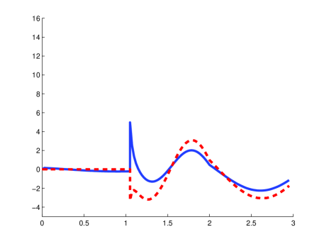
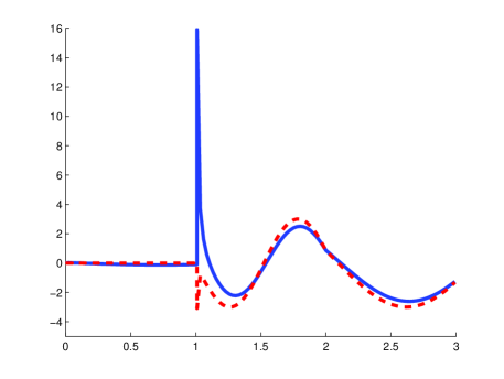
Figure 1: The $\theta$-component of the total $B$-field on the line $\{(x,0,0):\ x\in[0,3]\}$. Blue solid line correspond the field with no physical lining at $\{r=R\}$. Red dashed line correspond the field with Soft-and-Hard lining on $\{r=R\}$. At the left figure, the maximal anisotropy ratio is $L=1600$ and $R=1.05$. At the right figure, the maximal anisotropy ratio is $L=40,000$ and $R=1.01$.

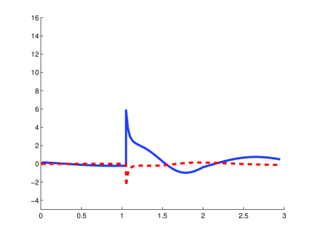
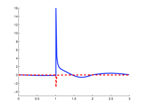
Figure 2: The $\theta$-component of the scattered $B$-field on the line $\{(x,0,0):\ x\in[0,3]\}$. Blue solid line correspond the field with no physical lining at $\{r=R\}$. Red dashed line correspond the field with Soft-and-Hard lining on $\{r=R\}$. At the left figure, the maximal anisotropy ratio is $L=1600$ and $R=1.05$. At the right figure, the maximal anisotropy ratio is $L=40,000$ and $R=1.01$.

5 Discussion

5.1 Comparison of results with and without SHS.

One observes that, without the SHS lining, the $B$-field grows as the approximate single coating tends more closely to the ideal invisibility cloak, i.e., as the anisotropy ratio $L$ becomes larger. In both Figs. 1 and 2, the peak near $r=1$ without the SHS lining shows quite clearly how the delta-distribution in the $B$-field develops.

Note that the value of the anisotropy ratio $L$ is quite large in our simulation, but the resulting fields are still not extremely large. So, it is not surprising that the non-existence results in [6], predicting the blow up of the fields, were not observed in the experiment [8]. However, it seems likely to become more significant as cloaking technology develops. Also, the SHS boundary lining has the additional benefit in our simulations of making the scattered wave smaller outside of the metamaterial construction. Indeed, the scattered field when using the SHS boundary lining is less than 2% of the scattered field without the lining. Thus, implementation of a lining significantly improves the cloaking effect.

5.2 Significance of the surface currents $\widetilde{J}_{surf}$ and $\widetilde{K}_{surf}$

As $R\to 1^{+}$, for generic incoming waves the magnetic and electric flux densities converge to fields that contain delta-function type distributional components supported on the surface $\Sigma$. We phrase this by saying that surface currents appear. If the metamaterial construction allows this, then we interpret this literally. This holds, e.g., if the metamaterials used have components near $\Sigma$ that approximate a SHS surface, such as strips of PEC and PMC materials. Alternatively, if no such currents can appear in the material, the $\widetilde{D}$ and $\widetilde{B}$ fields will blow up as the approximation of the coating material goes to the limit $R\to 1^{+}$.

Effective medium theory for composite materials is proven only when the limiting fields are relatively smooth [28]. Such rigorous effective medium theory has not yet been established for metamaterials, but the limited work so far, e.g., [29], clearly indicate that this same restriction will hold there as well. One can then interpret the blow up of fields as a challenge to the validity of the material parameters that have been ascribed to the metamaterilas currently employed. Indeed, fields having a blow up are very rapidly changing functions near the cloaking surface. Thus making a physical cloaking construction that would operate well with such fields would require metamaterials whose cell size becomes very small close to the cloaking surface.

The simplest way to avoid these issues would be to include the SHS lining when constructing the cloaking device.

5.3 Summary

We have considered two cases when cloaking an infinite cylinder:

(1) An infinite cylinder of air or vacuum, is coated with metamaterial in $\{R<r<2\}$ but has no lining on the interior surface of the metamaterial coating. In the limit $R\to 1^{+}$, solutions to Maxwell’s equations have singular current terms $K_{surf}$ and $J_{surf}$ that represent either surface currents or the blow up of the $D$ and $B$ fields. A standard assumption in homogenization theory is that the length scale, $d$, of the substructures (or cells) from which a composite medium is formed, is much less than the free space wavelentgnt $\lambda$ of the EM field [28]. In treatments of homogenization for metamaterials, e.g., [29], it has been observed that effective material parameters can often be obtained even when $d$ is not greatly less than $\lambda$. Although not explicitly stated, it is required that sampled surface intergrals of $E,H,B$, and $D$ not vary greatly from point to point within a metamaterial cell. The blow up of $B$ that we have shown occurs when cloaking wihout an SHS lining thus presents a challenge to the effective medium intepretation of the metamaterials employed.

(2) An infinite cylinder of air or vacuum is coated with metamaterial in $\{R<r<2\}$ and a SHS-lining on the interior of the cloaking surface. The lining can be considered as parallel PEC and PMC strips, that allow surface currents in the $z$-directions. In this case, when $R\to 1^{+}$, the total $E$ and $H$ fields at the boundary have very small $\theta$-components, that is, in the limit the tangent components of $E$ and $H$ are $z$-directional. The non-zero tangential boundary values of $E$ and $H$ correspond physically to surface currents, that are now allowed because of the SHS lining. Since the surface lining and fields are now compatible, the fields do not blow up. In addition, the amplitude of the farfield pattern is greatly reduced.

Department of Mathematics

University of Rochester

Rochester, NY 14627, USA

Email:allan@math.rochester.edu

Department of Mathematical Sciences

University of Loughborough

Loughborough, LE11 3TU, UK

Email:Y.V.Kurylev@lboro.ac.uk

Institute of Mathematics

Helsinki University of Technology

Espoo, FIN-02015, Finland

Email:Matti.Lassas@tkk.fi

Department of Mathematics

University of Washington

Seattle, WA 98195, USA

Email:gunther@math.washington.edu

Acknowledgements: A.G. was supported by NSF-DMS; M.L. by CoE-program 213476 of the Academy of Finland; and G.U. by NSF-DMS and a Walker Family Endowed Professorship.

References

• [1] A. Greenleaf, M. Lassas and G. Uhlmann, Anisotropic conductivities that cannot detected in EIT, Physiological Measurement (special issue on Impedance Tomography), 24 (2003), pp. 413-420.
• [2] A. Greenleaf, M. Lassas and G. Uhlmann, On nonuniqueness for Calderón’s inverse problem, Math. Res. Let. 10 (2003), no. 5-6, 685-693.
• [3] U. Leonhardt, Optical conformal mapping, Science 312 (23 June, 2006), 1777-1780.
• [4] J.B. Pendry, D. Schurig and D.R. Smith, Controlling electromagnetic fields, Science 312 (23 June, 2006), 1780-1782.
• [5] J.B. Pendry, D. Schurig, D.R. Smith, Calculation of material properties and ray tracing in transformation media, Optics Express 14 (2006), 9794.
• [6] A. Greenleaf, Y. Kurylev, M. Lassas and G. Uhlmann, Full-wave invisibility of active devices at all frequencies, ArXiv.org:math.AP/0611185v1,2,3, 2006; Comm. Math. Phys., to appear.
• [7] S. Cummer, B.-I. Popa, D. Schurig, D. Smith and J. Pendry, Full-wave simulations of electromagnetic cloaking structures, Phys Rev E 2006 Sep;74(3 Pt 2):036621.
• [8] D. Schurig, J. Mock, B. Justice, S. Cummer, J. Pendry, A. Starr and D. Smith, Metamaterial electromagnetic cloak at microwave frequencies, Science 314 (10 Nov. 2006), 977-980.
• [9] W. Cai, U. Chettiar, A. Kildshev and V. Shalaev, Optical cloaking with metamaterials, Nature Photonics, 1 (April, 2007), 224–227.
• [10] H. Chen and C.T. Chan, Transformation media that rotate electromagnetic fields, ArXiv.org:physics/0702050v1 (2007).
• [11] F. Zolla, S. Guenneau, A. Nicolet and J. Pendry, Electromagnetic analysis of cylindrical invisibility cloaks and the mirage effect, Optics Letters 32 (2007), 1069–1071.
• [12] G. Milton, M. Briane and J. Willis, On cloaking for elasticity and physical equations with a transformation invariant form, New J. Phys. 8 (2006), 248.
• [13] S. Cummer and D. Schurig, One path to acoustic cloaking, New Jour. Physics 9 (2007), 45.
• [14] G. Milton, New metamaterials with macroscopic behavior outside that of continuum elastodynamics, preprint, ArXiv.org:070.2202v1 (2007).
• [15] S. Schelkunoff and H. Friis, Antennas: Theory and Practice, Chapman and Hall, New York,1952, 584–585.
• [16] A. Moroz, Some negative refractive index material headlines…, http://www.wave-scattering.com/negative.html.
• [17] R. Weder, A rigorous time-domain analysis of full–wave electromagnetic cloaking (Invisibility), preprint, ArXiv.org:07040248v1,2,3 (2007).
• [18] A. Greenleaf, Y. Kurylev, M. Lassas and G. Uhlmann, Electromagnetic wormholes and virtual magnetic monopoles, ArXiv.org:math-ph/0703059, submitted, 2007.
• [19] A. Greenleaf, Y. Kurylev, M. Lassas and G. Uhlmann, Electromagnetic wormholes via handlebody constructions, ArXiv.org:0704.0914v1, submitted, 2007.
• [20] Z. Ruan, M. Yan, C. Neff and M. Qiu, Confirmation of cylindrical perfect invisibility cloak using Fourier-Bessel analysis, preprint, ArXiv.org:0704.1183v1 (2007).
• [21] M. Yan, Z. Ruan, and M. Qiu, Cylindrical invisibility cloak with simplified material parameters is inherently visible, preprint, ArXiv.org:0706.0655v1 (2007).
• [22] P.-S. Kildal, Definition of artificially soft and hard surfaces for electromagnetic waves, Electron. Lett. 24 (1988), 168–170.
• [23] P.-S. Kildal, Artificially soft-and-hard surfaces in electromagnetics, IEEE Trans. Ant. and Propag., 10 (1990), 1537-1544.
• [24] I. Hänninen, I. Lindell, and A. Sihvola, Realization of generalized Soft-and-Hard Boundary, Progr. In Electromag. Res., PIER 64, 317-333, 2006.
• [25] I.M. Gel’fand and G.E. Shilov, Generalized Functions, I-V, Academic Press, New York, 1964.
• [26] C. Colton and R. Kress, Inverse acoustic and electromagnetic scattering theory. Second edition. Applied Mathematical Sciences, 93. Springer-Verlag, Berlin, 1998.
• [27] M. Abramowitz, I. Stegun, Irene A. Handbook of mathematical functions with formulas, graphs, and mathematical tables., U.S. Government Printing Office, Washington, D.C.,1964.
• [28] G. Milton, The Theory of Composites, Cambridge U. Press, 2001.
• [29] D. Smith and J. Pendry, Homogenization of metamaterials by field averaging, J. Opt. Soc. Am., 23 (2006), 391–403.