Fluorescence during Doppler cooling of a single trapped atom

Abstract

We investigate the temporal dynamics of Doppler cooling of an initially hot single trapped atom in the weak binding regime using a semiclassical approach. We develop an analytical model for the simplest case of a single vibrational mode for a harmonic trap, and show how this model allows us to estimate the initial energy of the trapped particle by observing the fluorescence rate during the cooling process. The experimental implementation of this temperature measurement provides a way to measure atom heating rates by observing the temperature rise in the absence of cooling. This method is technically relatively simple compared to conventional sideband detection methods, and the two methods are in reasonable agreement. We also discuss the effects of RF micromotion, relevant for a trapped atomic ion, and the effect of coupling between the vibrational modes on the cooling dynamics.

Laser cooling of trapped neutral atoms and atomic ions is a well established technique: for example, cooling to the motional ground state Diedrich et al. (1989); Monroe et al. (1995); Perrin et al. (1998) and motional state tomography Leibfried et al. (1998) are routinely performed with resolved motional-sideband excitation techniques. Sideband techniques require the natural linewidth $\Gamma$ of the cooling transition to be small compared to the vibrational frequency of the trapped particle, in order to allow the motional sidebands to be resolved. Many experiments are, however, conducted in the “weak-binding regime”, where $\Gamma$ is larger than the oscillation frequency. Here, the cooling process is essentially the same as Doppler cooling of free atoms, because the spontaneous decay process is short compared to the atom’s oscillation period Wineland and Itano (1979). Even in experimental setups that implement sideband techniques, an initial stage of such “Doppler cooling” is often employed. The first examinations of Doppler cooling of trapped ions Wineland et al. (1978); Neuhauser et al. (1978); Wineland and Itano (1979); Javanainen and Stenholm (1980, 1981a, 1981b); Itano and Wineland (1982) did not take into account the effects of micromotion due to the trapping RF field. After cooling and heating effects related to micromotion were observed, these effects were explained theoretically Blümel et al. (1989); DeVoe et al. (1989); Cirac et al. (1994) by including the effects of micromotion.

Here, we consider Doppler cooling of a single trapped atom or ion. While most previous work has focused on the final stages of cooling, our focus will be on the temporal dynamics of the cooling, particularly in the “hot regime” where the Doppler shift due to atom motion is comparable to or much larger than $\Gamma$. For the 1-D case we find that the cooling rate can be calculated analytically in the weak-binding regime without assuming the atom to be in the Lamb-Dicke regime. For a trapped ion, when we take RF micromotion into consideration, stable, highly excited states emerge when only one mode is considered Peik et al. (1999). When all three vibrational modes of the ion are considered, we find that couplings between the modes tend to break the stability of such points allowing cooling to reach the Doppler limit.

A practical application of our results is to estimate the initial motional energy of an atom or ion from observations of the time dependence of the fluorescence during the cooling process. As mentioned above, sideband spectroscopy is the conventional technique for characterizing motional states, and it has been used to characterize the heating rate of ions in the absence of cooling Diedrich et al. (1989); Monroe et al. (1995); Turchette et al. (2000); Seidelin et al. (2006); Deslauriers et al. (2006); Pearson et al. (2006); Epstein et al. (2007). However, it is more complicated to implement experimentally than Doppler cooling, requiring more laser beams. Currently, considerable effort is being devoted to understanding the anomalous heating observed in ion traps Turchette et al. (2000); Seidelin et al. (2006); Deslauriers et al. (2006); Pearson et al. (2006); Epstein et al. (2007). A less complicated technique for measuring temperature could simplify this work.

This paper is structured as follows: In Sec. I we present a semiclassical model of the Doppler cooling process for a bound atom in the weak-binding regime. In Secs. II and III we analyze the fluorescence predicted by the model for a single vibrational mode unaffected by micromotion. Here, we consider single cooling trajectories and average over these with a given distribution of initial motional energies. We derive expressions useful for estimating initial temperature from fluorescence observations in these sections. Sec. IV discusses how to minimize the total measurement time required to estimate the mean initial energy. In Sec. V we consider the effects of other motional modes with and without taking into account any RF micromotion experienced by such modes. Sec. VI suggests modifications to the basic experimental protocol that might provide improved sensitivity of the temperature measurements. Sec. VII concludes the paper.

I Model

We consider a semiclassical model of Doppler cooling of a single weakly trapped atom Wineland and Itano (1979); Itano and Wineland (1982). We will initially consider only a single mode of motion, taken to be along the $z$ direction. We assume a harmonic potential with oscillation frequency $\omega_{z}$. In Sec. V we consider a more detailed model that includes three dimensions and micromotion for ions.

The atom is Doppler-cooled by a single laser beam of angular frequency $\nu_{\text{Laser}}$ and wave-vector $\bm{k}$, detuned by $\Delta\equiv\nu_{\text{Laser}}-\nu_{ge}$ from the resonance frequency $\nu_{ge}$ of a two-level, or “cycling”, transition between two internal states, $\left\lvert{\text{g}}\right\rangle$ and $\left\lvert{\text{e}}\right\rangle$, of the atom. We write the coupling Hamiltonian as

$$H^{({c})}=\hbar\,\Omega_{\text{Rabi}}\,\left(\left\lvert{\text{e}}\right\rangle\left\langle{\text{g}}\right\rvert+\left\lvert{\text{g}}\right\rangle\left\langle{\text{e}}\right\rvert\right)\,\cos(\bm{k}\cdot\bm{x}-\nu_{\text{Laser}}t),$$ (1)

where $\bm{x}$ is the atom position, $2\pi\hbar$ is Planck’s constant, and $\Omega_{\text{Rabi}}$ is the resonant Rabi frequency.

We assume the atom is weakly bound in the $z$ direction, that is, $\omega_{z}$ is much less than the excited state decay rate $\Gamma$. The atom’s level populations are then approximately in steady state with respect to the instantaneous effective detuning, $\Delta_{\text{eff}}\equiv\Delta+\Delta_{D}$, including the Doppler shift $\Delta_{D}\equiv-k_{z}v_{z}$, where $v_{z}$ and $k_{z}$ are the $z$-components of the velocity and wave-vector. The excited state population is then Loudon (1973)

$$\rho_{\text{ee}}(v_{z})=\frac{s/2}{1+s+(2\Delta_{\text{eff}}/\Gamma)^{2}}.$$ (2)

Here $s$ is the saturation parameter, proportional to the cooling beam intensity, $s\equiv 2|\Omega_{\text{Rabi}}|^{2}/\Gamma^{2}$.

The excited state population is associated with the photon scattering rate $dN/dt$ by the relation $dN/dt=\Gamma\rho_{\text{ee}}(v_{z})$. While the momentum kicks associated with photon emission are assumed to average to zero over many absorption-emission cycles, the absorbed photons will impart a velocity dependent momentum transfer due to the scattering that can be described by a velocity-dependent force

$$F_{z}(v_{z})=m\frac{dv_{z}}{dt}=\hbar k_{z}\,\Gamma\rho_{\text{ee}}(v_{z}),$$ (3)

where $m$ is the atom’s mass. This velocity-dependent force will in general change the motional energy $E$ of the atom. If the relative change in energy over a motional cycle is small, we can average the effect of $F_{z}$ over the oscillatory motion to find the evolution of $E$:

$$\frac{dE}{dt}=\left\langle v_{z}F_{z}(v_{z})\right\rangle,$$ (4)

where the average is over one motional cycle. The average energy change per scattering event is $dE/dN=\hbar k_{z}v_{z}=-\hbar\Delta_{D}$.

In addition to $F_{z}$, the atom will experience a stochastic force due to photon recoil that, assuming isotropic emission, will cause heating at a rate Itano and Wineland (1982)

$$\left(\frac{dE}{dt}\right)_{\text{recoil}}=\frac{4}{3}\frac{\left(\hbar\,k_{z}\right)^{2}}{2m}\,\frac{dN}{dt},$$ (5)

where $(\hbar k_{z})^{2}/2m$ is the recoil energy associated with the scattering. We will mostly ignore the effects of recoil heating in what follows since it will be important only near the cooling limit.

II Analysis

We will now analyze the time-dependence of the atom fluorescence during the Doppler cooling process, as predicted by the model introduced above.

To simplify the algebra, we will scale energies by $\hbar$ times half the power-broadened linewidth, and time by the resonant scattering rate:

$$\{\varepsilon,\delta,r\} =\{E,\hbar\Delta,\frac{(\hbar k_{z})^{2}}{2m}\}/E_{0}, E_{0} =\frac{\hbar\Gamma}{2}\sqrt{1+s}$$

$$\tau =t/t_{0}, t_{0} =\left(\Gamma\frac{s/2}{1+s}\right)^{-1}.$$

As an example of typical values, we consider a trapped ${}^{25}\text{Mg}^{+}$ ion, where the ${}^{2}S_{1/2}-^{2}P_{3/2}$ cooling transition at $279.6\,\text{nm}$ has a natural linewidth of $\Gamma=2\pi\times 41.4\,\text{MHz}$. At a detuning of $\Delta=-2\pi\times 20\,\text{MHz}$ with $s=0.9$ and $k_{z}/k=0.71$, we find that $E_{0}/k_{B}=1.4\,\text{mK}$, where $k_{B}$ is Boltzmann’s constant, and $t_{0}=16\,\text{ns}$. The detuning and recoil parameters are $\delta=-0.70$ and $r=0.0018$.

Figure 1: Scattering rate (top) and energy (bottom) as a function of time during the Doppler cooling of a single atom from an initial energy of $10/r$, as given by Eqs. (10a) and (II) at a detuning of half the power-broadened linewidth ($\delta=-1$). The dotted curve in the lower plot shows the energy predicted by the asymptotic approximation (12). Insets in the upper plot show (at two different times) the two components appearing in the integral defining $dN/d\tau$ in Eq. (II): The probability density of the effective detuning $P_{D}(\delta_{M};\delta_{\text{eff}}-\delta)$ (solid) and the Lorentzian line profile, $L(\delta_{\text{eff}})=1/(1+\delta_{\text{eff}}^{2})$ (dashed) as a function of $\delta_{\text{eff}}=\delta+\delta_{D}$ at $\varepsilon=8/r$ and $\varepsilon=\varepsilon_{s}$. Scattering events where the atom is moving towards the laser so that $\delta_{D}>0$, corresponding to the rightmost peak of $P_{D}$, result in cooling, and vice versa. The energies of maximal cooling and scattering rates, $\varepsilon_{c}$ and $\varepsilon_{s}$, are given by Eqs. (13) and (14).

The maximal change in energy per scattering event at a given energy is $\delta_{M}\equiv 2\sqrt{\varepsilon r}$. The energy at which the maximal Doppler shift, which in the scaled units is equal to $\delta_{M}$, is equal to the power-broadened linewidth, $\delta_{M}=2$, is of interest during the cooling process. For reference we note that this energy corresponds to

$$\frac{1}{r}\,E_{0}=(1+s)\frac{\hbar^{2}\Gamma^{2}}{4}\frac{2m}{\hbar^{2}k_{z}^{2}}.$$ (7)

For the typical experimental parameters considered above, $E_{0}/r$ is equal to $k_{B}\times 700\,\text{mK}$ or $3700\,\hbar\omega_{z}$ for $\omega_{z}=2\pi\times 4.0\,\text{MHz}$.

For harmonic oscillations, the instantaneous Doppler shift $\delta_{D}\equiv\hbar\Delta_{D}/E_{0}$ is distributed according to the probability density

$$P_{D}(\delta_{M};\delta_{D}) =\int_{0}^{2\pi}\delta_{\text{Dirac}}(\delta_{D}-\delta_{M}\sin(\phi))\,\frac{d\phi}{2\pi}$$

$$=\begin{cases}\frac{1}{\pi}\frac{1}{\sqrt{\delta_{M}^{2}-\delta_{D}^{2}}}&\text{if }\lvert\delta_{D}\rvert<\delta_{M},\\ 0&\text{otherwise,}\end{cases}$$ (8)

where $\delta_{\text{Dirac}}$ is the Dirac $\delta$ function. Since the average energy change per scattering event is $-\delta_{D}$, and the instantaneous scattering rate is $1/(1+\delta_{\text{eff}}^{2})$, where $\delta_{\text{eff}}\equiv\delta+\delta_{D}$, the rate of change of $\varepsilon$ averaged over the secular oscillations by Eq. (4) takes the form:

$$\frac{d\varepsilon}{d\tau}=\int-\delta_{D}P_{D}(\delta_{M};\delta_{D})\frac{1}{1+(\delta+\delta_{D})^{2}}d\delta_{D},$$ (9)

as illustrated in Fig. 1. We can evaluate the integral as detailed in Appendix A, to find that

$$\frac{d\varepsilon}{d\tau} =\frac{1}{2\sqrt{\varepsilon r}}(\operatorname*{Re}(Z)+\delta\operatorname*{Im}(Z))$$ (10a)

$$\approx\frac{\delta}{2\sqrt{\varepsilon r}},\quad\varepsilon\gg(1+\delta^{2})/r,$$ (10b)

where $Z=Z(\delta,\delta_{M})=i/\sqrt{1-(\delta+i)^{2}/4\varepsilon r}$. The asymptotic approximation (10b) corresponds to approximating $P_{D}(\delta_{M};\delta_{D})$ by $P_{D}(\delta_{M};0)$, which is reasonable in the “hot” regime, where the peaks of $P_{D}$ have small overlap with the Lorentz line profile.

The scattering rate averaged over the motion is analogous to Eq. (10) and is given by

$$\frac{dN}{d\tau} =\int P_{D}(\delta_{M};\delta_{D})\frac{1}{1+(\delta+\delta_{D})^{2}}d\delta_{D}$$

$$=\frac{1}{2\sqrt{\varepsilon r}}\operatorname*{Im}(Z),$$ (11)

as illustrated in Fig. 1. In the limit of $\varepsilon\gg(1+\delta^{2})/r$, we find $dN/d\tau\approx 1/(2\sqrt{\varepsilon r})$, so that according to Eq. (10b) we have in this limit $d\varepsilon/dN\approx\delta$. This corresponds to each photon on average extracting an energy of $\hbar\Delta$. This can be understood by noting that in the limit of $\varepsilon\gg(1+\delta^{2})/r$, $P_{D}(\delta_{M};\delta_{D})$ is to a good approximation uniform over the Lorentz line profile, and so the value of $\delta_{\text{eff}}=\delta+\delta_{D}$ averaged over the scattering events will be zero. Since each scattering event extracts an energy of $-\delta_{D}$, the average cooling per scattering event should indeed be $\delta$.

Figure 2: The scattering rate, $dN/d\tau$, vs. time during Doppler cooling of a single atom with initial energy $\varepsilon=10/r$ for different laser detunings. For $\delta<\delta_{C}=-1/\sqrt{3}$, a maximal scattering rate occurs at $\varepsilon=\varepsilon_{s}$, as given by Eq. (14). The maximal value of the scattering rate is given by Eq. (15). Closer to resonance, the scattering rate increases monotonically during the cooling.

The time-dependence of $\varepsilon$ is formally found by integrating $d\varepsilon/d\tau$ as given by Eq. (10). For the asymptotic approximation (10b) we find

$$\varepsilon(\tau)\approx\left(\varepsilon_{0}^{3/2}+\frac{3\delta\tau}{4\sqrt{r}}\right)^{2/3},\quad\varepsilon\gg(1+\delta^{2})/r,$$ (12)

where $\varepsilon_{0}$ is the energy at $\tau=0$, as plotted in the lower part of Fig. 1. For the exact expression (10a), we must resort to numerical methods, although we do find analytically that the cooling rate is maximal for $\varepsilon$ related to $\delta$ by

$$\varepsilon_{c}=\frac{1+\delta^{2}}{2r}\cos(\frac{1}{3}\arccos(\frac{1-\delta^{2}}{1+\delta^{2}})),$$ (13)

which quantifies our previous observation that $1/r$ is a typical energy scale of the cooling process.

The behavior of $dN/d\tau$ is qualitatively different for $\delta$ being smaller or larger than a critical detuning, $\delta_{C}\equiv-1/\sqrt{3}$. For $\delta<\delta_{C}$, $dN/d\tau$ has a maximum at

$$\varepsilon_{s}=\frac{1}{4r}(\delta-\sqrt{3})(\delta+1/\sqrt{3}).$$ (14)

For the example parameters listed below Eq. (6), $\delta_{C}$ corresponds to a detuning of $\delta_{C}E_{0}/\hbar=-2\pi\times 16.5\,\text{MHz}$. Closer to resonance, i.e., when $\delta_{C}<\delta<0$, no maximum occurs, as illustrated in Fig. 2. The maximal scattering rate is reached when one of the peaks of the Doppler distribution (II) is in resonance with the cooling transition, as illustrated in the insets of Fig. 1. In the regime where a maximum exists, the maximal scattering rate is found to exceed the steady state scattering rate by a factor of

$$\left.\frac{dN}{d\tau}\right\lvert_{\varepsilon=\varepsilon_{s}}/\left.\frac{dN}{d\tau}\right\lvert_{\varepsilon=0}=\frac{\sqrt{3\sqrt{3}}}{4}\frac{1+\delta^{2}}{\sqrt{|\delta|}}.$$ (15)

We emphasize that the only approximations made above are the weak-binding approximation and the omission of recoil heating. In particular, the trapped particle is not assumed to be in the Lamb-Dicke regime. For the weak-binding regime, $\delta_{M}>1$ implies that the motion is well outside the Lamb-Dicke regime. To find the cooling rate predicted by (10) in the Lamb-Dicke limit, we note that to first order in $\varepsilon$ we have $d\varepsilon/d\tau\approx 4\delta\varepsilon r/(1+\delta^{2})^{2}$. This corresponds to $\varepsilon$ decreasing exponentially with $\tau$. Except for the omission of recoil heating, the value of the decay time agrees with previous work that assumed the atom was in the Lamb-Dicke regime Wineland and Itano (1979); Wells and Cook (1990).

In the above analysis, we have ignored recoil heating as given by Eq. (5). In the limit of $\varepsilon\gg\varepsilon_{c}$, the ratio of heating to cooling is seen to be $4r/(3|\delta|)$, which is a small fraction for realistic parameters. For $\varepsilon<\varepsilon_{c}$, the cooling is less efficient and the contribution from recoil becomes more significant, leading to a nonzero steady-state energy. Nevertheless, ignoring recoil heating is reasonable when considering only fluorescence, since the scattering rate has almost reached its steady-state value when the effect of recoil becomes important. We have omitted recoil in this analysis to make $\delta$ the only free parameter and simplify the discussion. Recoil can be included in calculations by combining Eqs. (5), (10a), and (II).

III Thermal averaging

An application of the analysis presented above is to estimate the initial motional energy of a trapped atom from the fluorescence observed during the cooling process. Using this method, we can estimate the average rate of heating experienced by a trapped atom in the absence of cooling by first allowing the atom to heat up without cooling for a certain period and then observing the time dependence of the fluorescence as the atom is re-cooled. As discussed in Sec. II, we have for $\varepsilon\gg(1+\delta^{2})/r$ that the average cooling per scattering event is $\delta$. The approximate total number of photons scattered during the cooling of an atom with initial motional energy $\varepsilon_{\text{initial}}$ can consequently be approximated by $\lvert\varepsilon_{\text{initial}}/\delta\rvert$. For the example parameters given in Sec. II, this corresponds to $\approx 800$ photons for $\varepsilon_{\text{initial}}=1/r$, corresponding to $k_{B}\times 700\,\text{mK}$. With typical photon detection efficiencies of less than $10^{-3}$, very few photons are registered in a single experiment. We must therefore repeat many experimental cycles consisting of a heating period and a cooling period.

We now consider the form of the fluorescence signal when averaged over many such experimental cycles. Here, we will assume the heating is stochastic and take the distribution $P_{0}(\varepsilon)$ of the motional energies at the beginning of each cooling period to be the Maxwell-Boltzmann distribution with mean energy $\bar{\varepsilon}$,

$$P_{0}(\varepsilon)=\tfrac{1}{\bar{\varepsilon}}\,e^{-\varepsilon/\bar{\varepsilon}}.$$ (16)

However, the results below hold for any form of $P_{0}(\varepsilon)$.

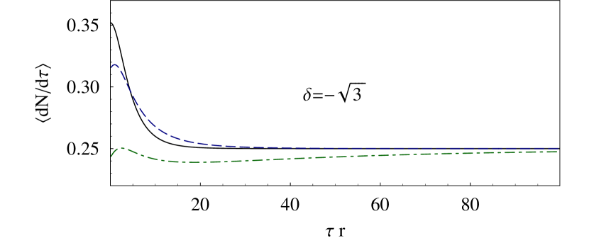
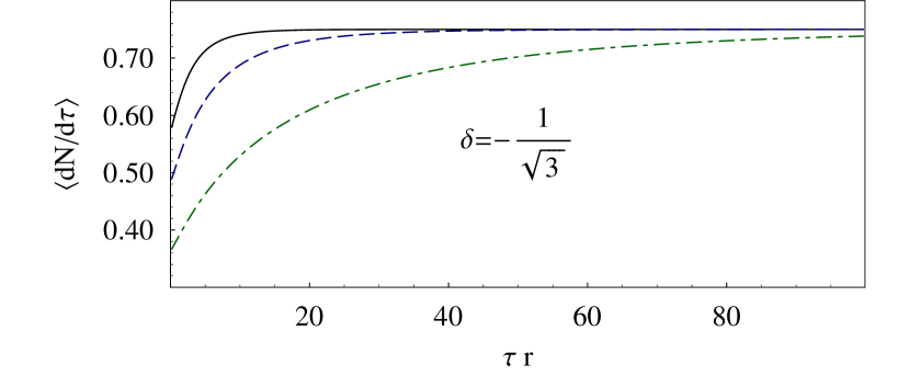
Figure 3: Thermally averaged scattering rate vs. time, for $\delta=-\sqrt{3}$ (top) and $\delta=-1/\sqrt{3}=\delta_{C}$ (bottom). In both figures, $P_{0}$ is assumed to be a thermal distribution with $\bar{\varepsilon}$ equal to $1$,$2$, and $4$ times $\varepsilon_{c}$ for the solid, dashed, and dash-dotted lines respectively. Note that for $\delta<\delta_{C}$, the initial fluorescence is larger than the steady-state fluorescence for low values of $\bar{\varepsilon}$; this is attributed to the local maximum in the fluorescence illustrated in Fig. 2.

The thermally averaged scattering rate is conveniently written in terms of the propagator, $\Xi$, of $\varepsilon$: Let $\Xi(\varepsilon_{0},\tau)$ denote the energy at time $\tau$ of an atom with initial energy $\varepsilon(\tau=0)=\varepsilon_{0}$. We can then write the thermally averaged scattering rate at time $\tau$ as

$$\left\langle\frac{dN}{d\tau}\right\rangle_{\bar{\varepsilon}}=\int_{0}^{\infty}P_{0}(\varepsilon^{\prime})\left.\frac{dN}{d\tau}\right|_{\varepsilon=\Xi(\varepsilon^{\prime},\tau)}d\varepsilon^{\prime}.$$ (17)

This can be efficiently computed numerically by noting that $\Xi(\Xi(\varepsilon,\tau_{1}),\tau_{2})=\Xi(\varepsilon,\tau_{1}+\tau_{2})$, as detailed in Appendix B. Figure 3 shows the thermally averaged scattering rate for a few different parameters.

Figure 4: Experimentally observed fluorescence during Doppler cooling of a single $\text{Mg}^{+}$ ion compared with the fluorescence predicted by the simple 1-D model. Data points (triangles) indicate the observed scattering rates, obtained by integrating over many experiments. In each experiment, the time-resolved fluorescence is recorded while the ion is re-cooling after having been allowed to heat up for a period of $25\,\text{s}$. The experimental parameters were those given after Eq. (6). Error bars are based on counting statistics. The solid curve is the scattering rate predicted by Eq. (17), assuming the motional energy of the ion after the heating period to be given the Maxwell-Boltzmann distribution (16) with $\bar{\varepsilon}=5.1/r$, corresponding to a temperature of $3.9\,\text{K}$. Since $\bar{\varepsilon}$ is the only free parameter of Eq. (17), the estimated value was extracted by a single parameter fit, and agrees reasonably well with an independent temperature estimate of $3.4\pm 0.3\,\text{K}$ extrapolated from heating rates measured in the same trap by use of the Raman sideband technique Epstein et al. (2007).

The fluorescence predicted by Eq. (17) has been found to be in good agreement with experimentally observed fluorescence. We show one experimental data set for comparison in Fig. 4; the experiments are more fully described in Epstein et al. (2007). Furthermore, the resulting estimated heating rates have been found to agree well with results obtained using the Raman sideband technique Seidelin et al. (2006); Epstein et al. (2007). This agreement may at first seem surprising, given that the two methods probe very different energy scales. For the measurements based on the Raman sideband technique the ion was only allowed to heat for a few milliseconds thereby gaining a few motional quanta while the measurement results presented in Fig. 4 are based on $25\,\text{s}$ heating periods allowing the ion to gain many motional quanta. However, the results should agree if, as expected, the heating rate is constant over these energy scales.

IV Optimal experimental parameters

We now examine how the total measurement time required to reach a given accuracy on the heating rate estimate depends on the choice of experimental parameters. As the recoil parameter $r$ will be fixed by choice of atom, we consider only the choice of optimal values for $\bar{\varepsilon}$, $\delta$, and laser beam intensity.

It is clear from Fig. 2 that the relevant size of the signal, in terms of fluorescence photons emitted, for a given initial motional energy increases with decreasing detuning: the re-cooling is slower and the change in scattering rate is larger. For a given experimental setup, the optimal detuning is decided as a compromise between re-cooling signal and ability to re-cool atoms that have been highly excited by e.g., collisions.

For a given value of $\bar{\varepsilon}$, the experimental signal, in terms of the number of photons scattered before steady state is reached, does not depend on the laser beam intensity. Since $\bar{\varepsilon}$ is the average initial energy relative to $E_{0}$, which is proportional to the power-broadened linewidth, a lower laser beam intensity will give a larger signal for a given heating period. This suggests using the smallest feasible laser intensity, requiring a compromise with respect to robust cooling and detector dark counts. From this standpoint we want to keep the saturation parameter below, but probably close to, $1$.

For a given detuning and laser intensity, an additional choice of the length of the heating period in each experimental cycle has to be made: Should we perform a relatively low number of cycles with long heating periods or more cycles with shorter heating periods?

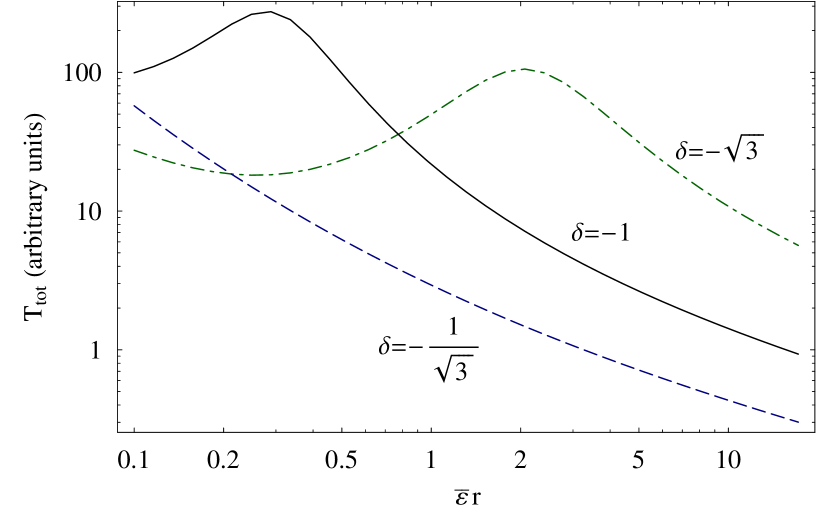
Figure 5: Total measurement time required to establish the heating rate with a given accuracy, assuming the integration time to be dominated by time for re-heating. A local maximum is observed for all detunings, but for $\delta=-1/\sqrt{3}$ it is located outside the range covered by the plot.

To answer this question, we estimate the total measurement time, $T_{\text{tot}}$, required to reach a certain relative accuracy on the estimate of the heating rate. We assume a constant heating rate and assume that the total time is dominated by the heating periods, so that $T_{\text{tot}}$ is proportional to the average initial energy, $\bar{E}\propto\bar{\varepsilon}\,\sqrt{1+s}$, and to the the number of runs.

We will consider a setup where the observed fluorescence is collected in sequential time-bins that are short compared to the total time required for the cooling process. In the limit where the distribution of the integrated number of counts, $n_{i}$, in time-bin $i$ is described by a normal distribution with variance $\sigma_{i}$, we can estimate the uncertainty on the maximum-likelihood estimate of $\bar{\varepsilon}$ for a given dataset by Press and William (1989)

$$1/\sigma(\bar{\varepsilon})^{2}=\sum_{i}\left(\frac{\partial n_{i}}{\partial\bar{\varepsilon}}\right)^{2}/\sigma_{i}^{2}.$$ (18)

It follows from Eqs. (10a), (II), and (17), that in the 1-D case the cooling dynamics can be rewritten in a form independent of $r$ by reparametrizing in terms of $Nr$, $\varepsilon r$, and $\tau r$. We will denote the reparametrized scattering rate by

$$\bar{R}_{\delta}(\bar{\varepsilon}r,\tau r)=\left\langle\frac{\partial(Nr)}{\partial(\tau r)}\right\rangle_{\bar{\varepsilon}r}.$$ (19)

Since the relative uncertainty on the heating rate estimate is equal to $\sigma(\bar{\varepsilon})/\bar{\varepsilon}$ and $\sigma_{i}=\sqrt{n_{i}}$, Eqs. (18) and (19) allow us to estimate the time required to obtain a given relative uncertainty on the heating rate:

$$\frac{T_{\text{tot}}}{\sqrt{1+s}}\propto\left(\bar{\varepsilon}r\int_{0}^{\infty}\left(\frac{\partial\bar{R}_{\delta}(\bar{\varepsilon}r,q)}{\partial\bar{\varepsilon}r}\right)^{2}\frac{dq}{\bar{R}_{\delta}(\bar{\varepsilon}r,q)}\right)^{-1}.$$ (20)

Note that the right hand side depends only on $\delta$ and $\bar{\varepsilon}r$. Fig. 5 shows $T_{\text{tot}}/\sqrt{1+s}$ calculated for different detunings. The figure confirms that a low detuning is indeed favorable, and also shows that for a given detuning, $T_{\text{tot}}$ decreases with increasing $\bar{\varepsilon}$. This is not surprising, given that the time to cool by a certain amount of energy increases with atom temperature, as illustrated by Fig. 1. It is clear from Fig. 5 that the heating period should be chosen long enough to get a significant signal, i.e., $\bar{\varepsilon}>\varepsilon_{c}$, but the optimal heating period must be decided based on other experimental parameters such as trap depth and background gas collision rate.

V Cooling in three dimensions

So far, we have considered only cooling in one dimension. In this section we will consider the effect of the vibrational modes in other directions on the cooling process. Our goal is to gain a qualitative understanding of the effects of the transverse modes on the cooling dynamics of the $z$ mode, with the intent of establishing to what extent the simple 1-D model presented above is a reasonable approximation.

V.1 3-D cooling of neutral atoms

For a neutral atom, the confinement transverse to $z$ is not associated with micromotion, as it is for ions, and the 1-D weak-binding model extends immediately to three dimensions. Let $\varepsilon_{i}$, $i=\{x,y,z\}$, denote the motional energy in mode $i$, $\delta_{D}^{({i})}=-\hbar k_{i}v_{i}/E_{0}$ the Doppler shift, and $\delta_{M}^{({i})}=2\sqrt{\varepsilon_{i}r_{i}}$ the maximum Doppler shift. Although all modes are formally identical in the absence of micromotion, we will discuss the cooling dynamics with a focus on the $z$ mode.

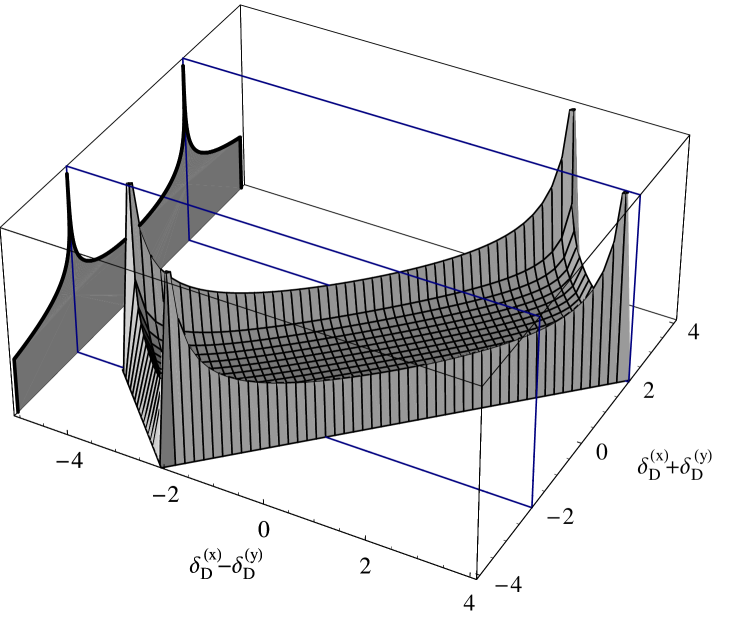
Figure 6: The probability density (22) for the combined Doppler shift $\delta_{D}^{\prime}=\delta_{D}^{({x})}+\delta_{D}^{({y})}$ due to two excited modes (curve on left wall) is a marginal distribution of the joint probability density $P_{D}(\delta_{M}^{({x})},\delta_{D}^{({x})})P_{D}(\delta_{M}^{({y})},\delta_{D}^{({y})})$ of $(\delta_{D}^{({x})},\delta_{D}^{({y})})$ (3-D surface). Note that only two of the peaks in the joint probability distribution lead to peaks in the marginal distribution. Plot is drawn for $\delta_{M}^{({x})}=3$ and $\delta_{M}^{({y})}=1$, as the dash-dotted line in Fig. 7, and the joint distribution is truncated to $|\delta_{D}^{({i})}|<0.95\,\delta_{M}^{({i})}$ for illustrational purposes.

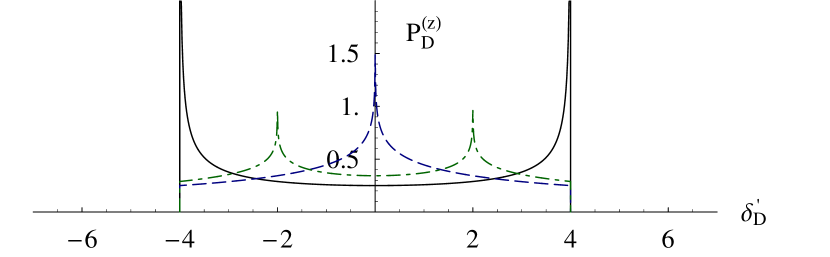
(a) (b)

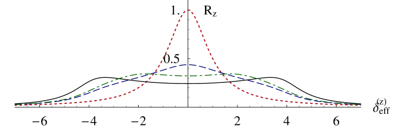
(c)

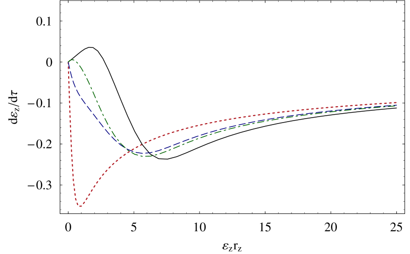
Figure 7: Cooling of the $z$ mode with two excited spectator modes in the absence of micromotion. Part (a) shows the probability density $P_{D}^{({z})}$ of the combined Doppler shift due to the $x$ and $y$ modes for $(\delta_{M}^{({x})},\delta_{M}^{({y})})$ equal to $(0,4)$ (solid), $(2,2)$ (dashed), and $(3,1)$ (dash-dotted). Part (b) shows the effective line profile $R_{z}(\delta_{\text{eff}}^{({z})})$ obtained by convolving $P_{D}^{({z})}$ with the Lorentz line profile. Here $\delta_{\text{eff}}^{({z})}=\delta+\delta_{D}^{({z})}$. The spectator mode parameters are the same as for (a), and the dotted line show the Lorentz line profile, corresponding to the spectator modes being cold, essentially the 1-D cooling case. Part (c) shows the $z$ mode cooling rate as a function of $\varepsilon_{z}$ for the effective line profiles of (b).

In experiments it is typically easy to make the frequencies of the three modes incommensurate, which we will assume here. In that case, we can write the rate of change of $\varepsilon_{z}$ as

$$\frac{d\varepsilon_{z}}{d\tau} =\int\frac{-\delta_{D}^{({z})}}{1+\left(\delta+\sum_{j}\delta_{D}^{({j})}\right)^{2}}\prod_{l}P_{D}(\delta_{M}^{({l})};\delta_{D}^{({l})})d^{3}\bm{\delta}_{D}$$

$$=\int-\delta_{D}^{({z})}P_{D}(\delta_{M}^{({z})};\delta_{D}^{({z})})R_{z}(\delta+\delta_{D}^{({z})})d\delta_{D}^{({z})},$$ (21)

where $R_{z}$ is the effective line profile experienced by the $z$ mode, obtained by convolving the Lorentz line profile with the distribution $P_{D}^{({z})}$ of the combined Doppler shift $\delta_{D}^{\prime}\equiv\delta_{D}^{({x})}+\delta_{D}^{({y})}$ due to the $x$ and $y$ “spectator” modes,

$$P_{D}^{({z})}(\delta_{D}^{\prime})=\int P_{D}(\delta_{M}^{({x})};u)P_{D}(\delta_{M}^{({y})};\delta_{D}^{\prime}-u)du.$$ (22)

As illustrated in Figs. 6 and 7, $P_{D}^{({z})}$ is peaked (diverges) at $\delta_{D}^{\prime}=\pm|\delta_{M}^{({x})}-\delta_{M}^{({y})}|$. If $|\delta_{M}^{({x})}-\delta_{M}^{({y})}|>2$, the peaks are separated by more than the width of the Lorentz profile, and $R_{z}$ will be double-peaked, as illustrated in Fig. 7. It follows from Eq. (V.1) that the cooling rate in the limit of small $\delta_{M}^{({z})}$ is proportional to the slope of $R_{z}$ at $\delta$, and that the rate of change of $\varepsilon_{z}$ is positive if the slope is negative. If $-|\delta_{M}^{({x})}-\delta_{M}^{({y})}|<\delta<0$, this will result in heating of the $z$ mode, at least as long as $\delta\pm\delta_{M}^{({z})}$ are both inside the peaks of $R_{z}$, i.e., while $\delta_{M}^{({z})}<|\delta_{M}^{({x})}-\delta_{M}^{({y})}|+\delta$, as illustrated in Fig. 7 for $(\delta_{M}^{({x})},\delta_{M}^{({y})})=(0,4)$ and $(1,3)$ DeVoe et al. (1989); Peik et al. (1999). The figure also shows that this thermalization or energy equilibration effect is not present if $|\delta_{M}^{({x})}-\delta_{M}^{({y})}|\lesssim 1$, as $R_{z}$ is not double-peaked in this case. Mathematically, $d\varepsilon_{z}/dt$, $R_{z}$, and $P_{D}^{({z})}$ are all conveniently expressed as convolution integrals of functions with known Fourier transforms.

The dashed lines in Fig. 8 show the cooling rates predicted by Eq. (V.1) for the case of only one excited spectator mode at different energies. When $\delta_{M}^{({z})}$ is large compared to $\delta_{M}^{({x})}$, we see that the cooling rate is almost unaffected by the spectator mode. This can be understood by noting that in the limit where $P_{D}(\delta_{M}^{({z})};\delta_{D}^{({z})})$ is uniform over the values of $\delta_{D}^{({z})}$ where $R_{z}(\delta+\delta_{D}^{({z})})$ is nonzero, the symmetry of $R_{z}$ implies that the average energy change per scattering event is $\delta$, as also discussed in Sec. II. Since $R_{z}(\delta_{\text{eff}})\approx 0$ for $\delta_{\text{eff}}>1+\delta_{M}^{({x})}+\delta_{M}^{({y})}$, this implies that the temperature of the spectator modes will not affect the cooling rate in this limit. At lower values of $\delta_{M}^{({z})}$, we generally see a decrease in the cooling rate in a gradual approach to the thermalization regime discussed above.

The consequences of thermalization/equilibration process are complex, when considering the full 3-D cooling problem. Consider for instance the case where only one mode is initially hot. According to the discussion above, this will result in heating of the two remaining modes, until the fastest heating mode has reached a value of $\delta_{M}$ similar to that of the initially hot mode. After this thermalization, the modes will be cooled simultaneously at a cooling rate significantly lower than the cooling rate for a single hot mode.

At this point, it is worth reconsidering the validity of our omission of recoil heating: The recoil heating rate as given by Eq. (5) is seen to have a maximum value of $4r/3$ at the resonant scattering rate. It is clear from Fig. 8 that for typical values of $r$ on the order of $10^{-3}$, recoil is insignificant at high energies.

(a)

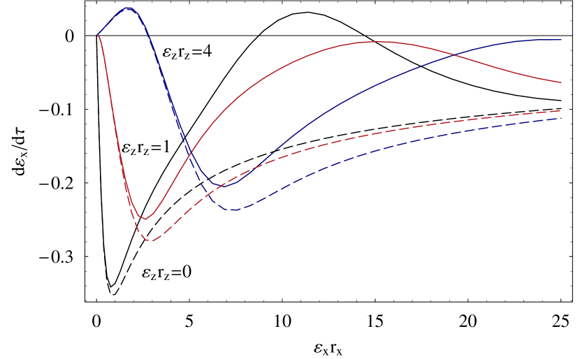
(b)

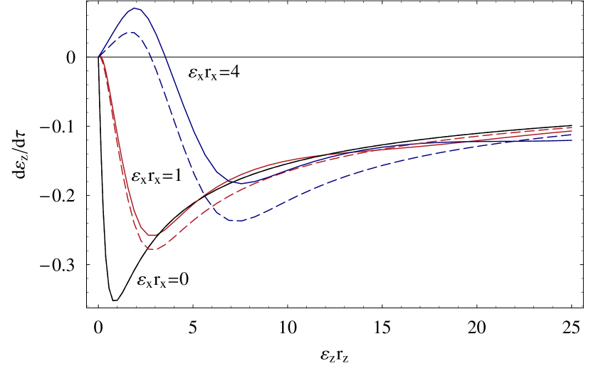
Figure 8: Predicted cooling rates for (a) a transverse mode in the presence of an excited $z$ mode and (b) the $z$ mode in the presence of a single excited transverse mode at $\delta=-1$. Dashed lines assume that the trapping potential has no associated micromotion, as described by Eq. (V.1). In this case, the cooling rates are of course identical for the two cases. The solid lines assume the transverse confinement to be provided by an RF quadrupole potential with a frequency $\tilde{\Omega}=6$, as described by Eq. (24). For both situations, the cooling rate is plotted with the spectator mode having a motional energy of $\varepsilon r=\{0,1,\text{and }4\}$. The plots are based on the weak binding model, and thus assume secular frequencies to be small compared to the linewidth. Note that the thermalization/equilibration effect discussed in the text is clearly observed for both cases.

V.2 3-D cooling of ions including the effects of micromotion

For an ion in a linear Paul trap, if we take the $z$ direction to be the axis, confinement in the transverse $x$ and $y$ directions is provided by the ponderomotive potential of an RF quadrupole field. The full 3-D cooling problem including micromotion on the transverse modes is very complex even in the Lamb-Dicke regime DeVoe et al. (1989); Walther (1993); Cirac et al. (1994). At low saturation, the effects of the micromotion caused by an RF field of frequency $\Omega$ can be modeled by including micromotion sidebands in the line profile DeVoe et al. (1989): Micromotion with peak amplitude $\bm{a}(\bar{\bm{x}}(t))$, where $\bar{\bm{x}}$ is the ion position averaged over one period of the RF field, can be described by the line profile,

$$R_{\mu}(\delta_{\text{eff}},\beta)=\sum_{n=-\infty}^{\infty}J_{n}^{2}(\beta)\,\frac{1}{1+(\delta_{\text{eff}}-n\tilde{\Omega})^{2}},$$ (23)

where $\delta_{\text{eff}}=\delta+\sum_{j}\delta_{D}^{({j})}$ is the effective detuning, $\beta=\left|\bm{a}(\bar{\bm{x}})\cdot\bm{k}\right|$ is the micromotion modulation index, $\tilde{\Omega}=\hbar\Omega/E_{0}$ is the scaled RF frequency, and $J_{n}$ is the $n$-th Bessel function.

In contrast to the situation in Ref. DeVoe et al. (1989), we are considering a case where $\beta$ changes during the secular motion. Since $\beta$ and $\delta_{\text{eff}}$ depend on $\bar{\bm{x}}$ and $\dot{\bar{\bm{x}}}$, respectively, we parametrize the secular motion by the instantaneous phases, $\phi_{i}$, where $\bar{x}_{i}=\bar{x}_{i}^{({0})}\cos(\phi_{i}(t))$, and where $\bar{x}_{i}^{({0})}$ is slowly varying and $\dot{\phi}_{i}\approx\omega_{i}$. Choosing the $x$ and $y$ axes so that the RF field is proportional to $(\bar{x}\hat{\bm{x}}-\bar{y}\hat{\bm{y}})\cos(\Omega t)$, we find that $\delta_{D}^{({i})}=\delta_{M}^{({i})}\sin(\phi_{i})$. In the limit where the transverse confinement is modified only weakly by static potentials, so that $\omega_{x}\approx\omega_{y}$, we find in the pseudopotential approximation that $\beta=\sqrt{2}\left|\delta_{M}^{({x})}\cos(\phi_{x})-\delta_{M}^{({y})}\cos(\phi_{y})\right|/\tilde{\Omega}$, which we note to be independent of the secular frequencies. In this case we have

$$\frac{d\varepsilon_{i}}{d\tau}=-\int\delta_{i}\,R_{\mu}(\delta_{\text{eff}}(\bm{\phi}),\beta(\phi_{x},\phi_{y}))\frac{d^{3}\bm{\phi}}{(2\pi)^{3}},$$ (24)

where the integral is over $[0,2\pi]$ in all dimensions. Note that since the modulation index depends only on the transverse components of the motion, the effect of excited transverse modes on the cooling of the $z$ mode can still be described in terms of an effective line profile, as in Eq. (V.1).

For the cooling of the transverse modes, the effects of micromotion on the cooling rates is pronounced, as illustrated by Fig. 8. A very clear qualitative difference from the cooling rate in the micromotion-free case is that at sufficiently high RF frequencies ($\tilde{\Omega}>4.4$ for $\delta=-1$), stable points for the transverse mode energies develop even when the remaining modes are cold. This effect has been discussed in Ref. Peik et al. (1999) and is attributed to the heating peak of the Doppler distribution becoming resonant with a micromotion sideband, as described by Eq. (23). This might be related to the bistable behavior reported in some single ion experiments Sauter et al. (1988a, b); Walther (1993). The stability breaks down when thermalization is taken into consideration. Consider for instance the stable point indicated by Fig. 8 to exist for $\bm{\varepsilon}\approx(15/r_{x},0,0)$. Here, it is clear from the figure that when the $z$ mode has heated to $\varepsilon_{z}>1/r_{z}$, cooling of the $x$ mode will commence.

When $\delta_{M}/\tilde{\Omega}\lesssim\sqrt{2}$ for the transverse modes, we find that only the $J_{0}$ term of Eq. (23) contributes significantly, and the argument of Sec. V.1 that the cooling rate for the $z$ mode is not affected by excited transverse modes when $\delta_{M}^{({z})}>1+\delta_{M}^{({x})}+\delta_{M}^{({y})}$ also applies here, as illustrated by Fig. 8.

It is clear from the results above that we cannot ignore the transverse modes if their associated maximal Doppler shifts are comparable to that of the $z$ mode. If, however, we assume the transverse modes are cold enough to avoid the heating effects described in Figs. 7 and 8, we have seen above that the primary effect of the transverse modes will be to slow down the cooling of the $z$ mode. This would result in the 1-D model overestimating the mean initial energy of the $z$ mode. However, for many experiments that use linear RF traps, it is reasonable to assume that the transverse modes are heated significantly less than the $z$ mode. This is because most investigations of the anomalous heating in ion traps have found the results to be consistent with heating rates having a frequency dependence of $\omega^{-n}$ with $n>1$ Turchette et al. (2000); Deslauriers et al. (2006); Epstein et al. (2007). Since the transverse mode frequencies are often an order of magnitude larger than $\omega_{z}$, this would indeed lead to the transverse modes being significantly colder than the $z$ mode. Also, since the energy in the transverse modes only affects the cooling of the $z$ mode through the resulting Doppler shift, the effect of the transverse modes could be further reduced by aligning $\bm{k}$ to have a smaller projection on the transverse modes. This would however reduce the efficiency of cooling of the transverse modes Itano and Wineland (1982).

Finally, another effect with respect to micromotion is that the presence of uncontrolled static stray fields can result in the ion experiencing micromotion even at the ion equilibrium position. At temperatures where $\delta_{M}\ll\tilde{\Omega}$, the first order effect according to Eq. (23) of this will be a reduction of the central spectral component by a factor of $J_{0}(\beta)^{2}$; see for example Ref. Berkeland et al. (1998). We note that this effect can be compensated by using an effective saturation parameter based on the steady-state fluorescence observed in the trap.

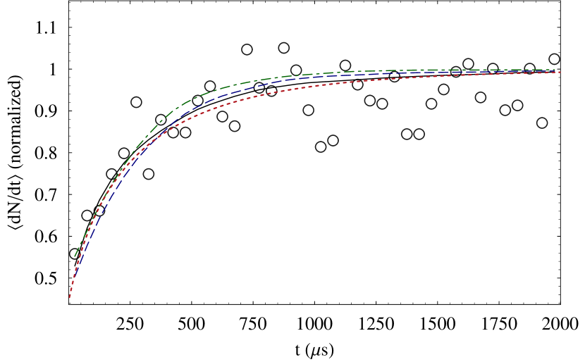
Figure 9: Averaged fluorescence vs. time as predicted by Monte Carlo simulations for best fits to the data presented in Fig. 4 for different models of the frequency dependence of the anomalous heating rate: The solid line assumes transverse modes to be unaffected by the heating; this should be very well approximated by the best fit to the 1-D model (dotted), as also plotted in Fig. 4. For the dashed and dash-dotted lines, we assume heating to be proportional to $\omega^{-1.4}$ and independent of $\omega$, respectively. The fitted value of the $z$ mode temperature for the three cases is $3.9\,\text{K}$, $3.7\,\text{K}$, and $1.4\,\text{K}$

V.3 Departures from the weak-binding, low-saturation limit

In most experimental situations, we will not strictly fulfill the requirements of low saturation or weak binding. In particular, for the trap referenced in Fig. 4 the secular frequencies of the transverse modes are approximately equal to half the $41.4\,\text{MHz}$ linewidth of the Doppler cooling transition, making the weak binding assumption only approximate. Also, the illustrated data were obtained at a saturation parameter of $0.9$, outside the validity region of the line-profile model that accounts for RF micromotion (24). To validate our claim that the fluorescence signal predicted by the 1-D model is a good approximation if the heating rate is assumed to be a strongly decreasing function of $\omega$, we performed a numerical Monte Carlo simulation of the fluorescence, based on integrating the optical Bloch equations through a large number of cooling trajectories. For each trajectory, we propagate the density matrix $\rho$ of the ion’s internal state according to the master equation

$$\frac{d\rho}{dt}=\frac{i}{\hbar}\left[\rho,H^{({c})}(\bm{x},t)\right]+2L\rho L^{\dagger}-\left\{L^{\dagger}L,\rho\right\},$$ (25)

where $L\equiv\left\lvert{\text{g}}\right\rangle\left\langle{\text{e}}\right\rvert\,\sqrt{\Gamma/2}$ is the Lindblad operator for excited state decay and $\bm{x}(t)=\bar{\bm{x}}(t)+\bm{a}(\bar{\bm{x}}(t))\cos(\Omega t)$ for the $\bar{\bm{x}}$ and $\bm{a}$ introduced above. Coupling to the motional state is modeled by the average light force, $m\ddot{\bar{\bm{x}}}=\hbar\bm{k}\,\Gamma\,\rho_{\text{ee}}(t)$. This model assumes neither the atoms to be weakly bound nor the cooling beam intensity to be low but does neglect recoil heating.

Figure 9 shows the result of fitting simulations with different assumptions for the frequency dependence of the heating to the dataset presented in Fig. 4. We find that if we assume the transverse modes are not heated, we obtain a temperature estimate of $3.9\,\text{K}$, in agreement with the result of fitting the 1-D model to the data, as illustrated by Fig. 4. The $z$ mode temperature of $3.7\,\text{K}$ estimated from the $\omega^{-1.4}$ model is close to, and slightly smaller than, this value, and agrees with the temperature estimate of $3.4\pm 0.3\,\text{K}$ based on extrapolating heating rates measured with the Raman sideband technique for the same trap configuration. This particular form of the frequency dependence of the heating rate was observed for the same trap when the Raman sideband technique Epstein et al. (2007) was used, and similar frequency dependencies have been observed in other geometries Turchette et al. (2000); Deslauriers et al. (2006). If we instead assume an $\omega^{-1}$ dependence of the heating, the results only change slightly.

Our main conclusions from the simulation results are that the primary effect of the presence of weakly heated spectator modes will be to slow down cooling due to thermalization. If $\omega^{-1.4}$ heating of the transverse modes is assumed, the 1-D model will somewhat overestimate the motional temperature of the axial mode.

VI Modified experimental protocols

We consider two modifications to the experimental protocol to reduce the total measurement time. Both are motivated by the fact that the size of the signal from a given amount of heating increases with increased initial energy.

One approach would be to coherently add a known amount of energy to the $z$ mode at the start of the heating period. If the added energy is enough to bring the atom into the slow-cooling regime, this will increase the signal change due to a given amount of additional heating, as illustrated in Fig. 10.

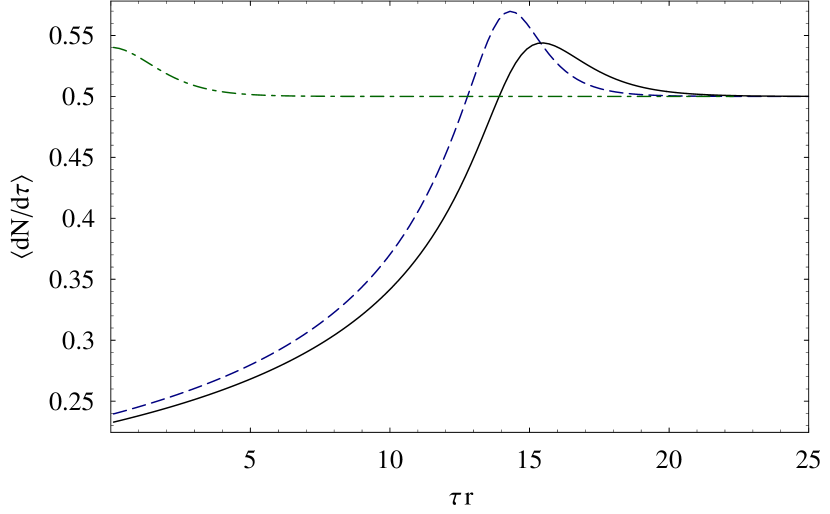
Figure 10: Improving the sensitivity of the temperature measurement by deliberate excitation. The dashed line shows the average scattering rate (17) as a function of time for an atom that was deliberately excited to a motional energy of $\varepsilon_{0}=5\varepsilon_{c}$, so that $P_{0}(\varepsilon)=\delta_{\text{Dirac}}(\varepsilon-\varepsilon_{0})$. The solid line shows the scattering rate as a function of time for an atom which has first been deliberately excited to a motional energy of $\varepsilon_{0}=5\varepsilon_{c}$ and then allowed to heat for a duration which added an average thermal energy of $\bar{\varepsilon}=0.25/r$. For comparison, the dash-dotted line shows the signal for an atom experiencing the same heating period without any initial excitation, i.e. with $\bar{\varepsilon}=0.25/r$. In all cases, $\delta=-1$.

Alternatively, parametric amplification Dehmelt and Walls (1968); Caves (1982); Heinzen and Wineland (1990) could be employed after the heating cycle to modify the thermal distribution. Parametric amplification can be implemented by modulating the $z$ trap potential at $2\omega_{z}$, and leads to amplification of one quadrature of the motion while damping the other quadrature. For a low value of $\bar{\varepsilon}$, parametric amplification would increase the fraction of experiments in which the atom is in the slow-cooling regime at the beginning of the cooling process, thus increasing the signal for a given heating period, as illustrated in Fig. 11.

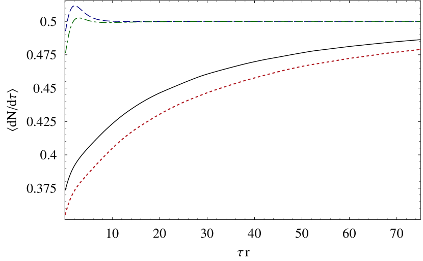
Figure 11: Improving the sensitivity of the temperature measurement by parametric amplification. The dashed and dash-dotted lines show the average scattering rate vs. time during the re-cooling of an atom which has been allowed to heat to $\bar{\varepsilon}=0.9\varepsilon_{c}$ and $1.1\varepsilon_{c}$ respectively at $\delta=-1$. The solid and dotted lines show the average scattering rate for the same conditions, except that the motional amplitude has been parametrically amplified by a factor of $3$ after the heating period.

VII Conclusion

In conclusion, we have shown that the motional energy of a trapped atom or ion can be estimated from the temporal changes in fluorescence observed when Doppler cooling is applied. Specifically, the initial energy can be estimated by fitting Eq. (17), where the mean initial motional energy is the only free variable, to the observed fluorescence. Our analysis assumes the oscillation frequency of the atoms is much smaller than the linewidth of the optical transition used for Doppler cooling and the motional energy at the start of the cooling is thermal.

Compared to Raman sideband transition methods for heating rate measurements, this method is simpler to implement experimentally but requires longer measurement duration for traps with low heating rates. On the other hand, for high heating rates, where sideband cooling is inefficient, this may be the method of choice. We have shown that in the typical situation, where the time for heating dominates, the total measurement time decreases with decreasing laser intensity, decreasing laser detuning, and increased heating period duration. We have compared the trade-off between these parameters (Fig. 5 and Eq. (20)). Finally, we show (Sec. IV) that the total measurement time can be reduced by adding additional energy to more quickly bring the ion into the low fluorescence regime.

By comparison with various models of 3-dimensional Doppler cooling, we have established that under typical experimental conditions the effects of the high-frequency modes are small, and that they will lead to temperature estimates that are somewhat higher than the actual temperature of the low-frequency mode.

Work supported by DTO and NIST. J.H.W. acknowledges support from The Danish Research Agency. R.J.E. acknowledges National Research Council Research Associateship Awards. S.S. acknowledges support from the Carlsberg Foundation. J.P.H. acknowledges support from a Lindemann Fellowship. We thank J. J. Bollinger and C. Ospelkaus for comments on the manuscript. This manuscript is a publication of NIST and is not subject to U.S. copyright.

Appendix A Integrals

The integrals appearing in Eqs. (9), (II), and (V.1) are all convolution integrals of elements with analytical Fourier transforms and can thus be easily evaluated in Fourier space. For the 1-D integrals, the inverse Fourier transform can also be performed analytically. Here we present a more direct approach to evaluating the 1-D integrals.

For $a,b\in\mathbb{R}$ we define $Z(a,b)$ as

$$Z\equiv\int_{0}^{2\pi}\frac{1}{\sin(\phi)-z}\frac{d\phi}{2\pi}=-\frac{1}{z}\,\sqrt{\frac{z^{2}}{z^{2}-1}},$$ (26)

where $z=(a+i)/b$. Noting that

$$\frac{1}{x-z}=b\frac{1}{1+(a-bx)^{2}}\left((bx-a)+i\right),$$ (27)

we find that, according to Eq. (26),

$$\int^{2\pi}_{0}\frac{b\sin(\phi)}{1+(a-b\sin(\phi))^{2}}\frac{d\phi}{2\pi} =\frac{1}{b}\,\left(\operatorname*{Re}(Z)+a\operatorname*{Im}(Z)\right)$$

$$\int^{2\pi}_{0}\frac{1}{1+(a-b\sin(\phi))^{2}}\frac{d\phi}{2\pi} =\frac{1}{b}\,\operatorname*{Im}(Z).$$

Taking the branch cut discontinuity for $\sqrt{\cdot}$ to be along the negative real axis, we have for $b>0$ that $\sqrt{(-iz)^{2}}=-iz$, so that

$$Z(a,b)=\frac{ib}{\sqrt{b^{2}-(a+i)^{2}}},\qquad b>0.$$ (28)

Appendix B Numerical calculation of the averaged scattering rate

In this section we present an efficient numerical method for evaluating the averaged scattering rate given by Eq. (17).

Introducing $\varepsilon_{n}=\Xi(\varepsilon_{0},n\Delta\tau)$, for $n=0,1,\ldots$, we note that $\Xi(\varepsilon_{m},n\Delta\tau)=\varepsilon_{m+n}$. The values of $\varepsilon_{n}$ are the energies along a single cooling trajectory. If the scattering rate can be considered constant on time scales of $\Delta\tau$,

$$\frac{dN}{d\tau}(\Xi(\varepsilon_{0},\tau))\approx R_{n},\qquad\tau\in[(n-1)\Delta\tau,n\Delta\tau],$$ (29)

we find that the thermally averaged scattering rate, as given by Eq. (17), averaged over the same intervals can be approximated by

$$\bar{R}_{n}\approx\sum_{m=0}^{\infty}R_{m+n}\ \int_{\varepsilon_{m}}^{\varepsilon_{m+1}}P_{0}(\varepsilon^{\prime})d\varepsilon^{\prime}.$$ (30)

Since the values of the $R_{n}$ are independent of $P_{0}$, $\bar{R}_{n}$ is easily calculated for different $P_{0}$ by list convolution.

For the Maxwell-Boltzmann distribution, a numerically stable form of the weight factors appearing in (30) is

$$\int_{\varepsilon-\Delta\varepsilon/2}^{\varepsilon+\Delta\varepsilon/2}e^{-\varepsilon^{\prime}/\bar{\varepsilon}}\frac{d\varepsilon^{\prime}}{\bar{\varepsilon}}=2e^{-\varepsilon/\bar{\varepsilon}}\sinh\left(\frac{\Delta\varepsilon}{2\bar{\varepsilon}}\right).$$

References

- Diedrich et al. (1989) F. Diedrich, J. C. Bergquist, W. M. Itano, and D. J. Wineland, Phys. Rev. Lett. 62, 403 (1989).
- Monroe et al. (1995) C. Monroe, D. M. Meekhof, B. E. King, S. R. Jefferts, W. M. Itano, D. J. Wineland, and P. Gould, Phys. Rev. Lett. 75, 4011 (1995).
- Perrin et al. (1998) H. Perrin, A. Kuhn, I. Bouchoule, and C. Salomon, Europhys. Lett. 42, 395 (1998).
- Leibfried et al. (1998) D. Leibfried, T. Pfau, and C. Monroe, Phys. Today 51, 22 (1998).
- Wineland and Itano (1979) D. J. Wineland and W. M. Itano, Phys. Rev. A 20, 1521 (1979).
- Wineland et al. (1978) D. J. Wineland, R. E. Drullinger, and F. L. Walls, Phys. Rev. Lett. 40, 1639 (1978).
- Neuhauser et al. (1978) W. Neuhauser, M. Hohenstatt, P. Toschek, and H. Dehmelt, Phys. Rev. Lett. 41, 233 (1978).
- Javanainen and Stenholm (1980) J. Javanainen and S. Stenholm, Appl. Phys. 21, 283 (1980).
- Javanainen and Stenholm (1981a) J. Javanainen and S. Stenholm, Appl. Phys. 24, 71 (1981a).
- Javanainen and Stenholm (1981b) J. Javanainen and S. Stenholm, Appl. Phys. 24, 151 (1981b).
- Itano and Wineland (1982) W. M. Itano and D. J. Wineland, Phys. Rev. A 25, 35 (1982).
- Blümel et al. (1989) R. Blümel, C. Kappler, W. Quint, and H. Walther, Phys. Rev. A 40, 808 (1989).
- DeVoe et al. (1989) R. G. DeVoe, J. Hoffnagle, and R. G. Brewer, Phys. Rev. A 39, 4362 (1989).
- Cirac et al. (1994) J. I. Cirac, L. J. Garay, R. Blatt, A. S. Parkins, and P. Zoller, Phys. Rev. A 49, 421 (1994).
- Peik et al. (1999) E. Peik, J. Abel, T. Becker, J. von Zanthier, and H. Walther, Phys. Rev. A 60, 439 (1999).
- Turchette et al. (2000) Q. A. Turchette, D. Kielpinski, B. E. King, D. Leibfried, D. M. Meekhof, C. J. Myatt, M. A. Rowe, C. A. Sackett, C. S. Wood, W. M. Itano, et al., Phys. Rev. A 61, 63418 (2000).
- Seidelin et al. (2006) S. Seidelin, J. Chiaverini, R. Reichle, J. J. Bollinger, D. Leibfried, J. Britton, J. H. Wesenberg, R. B. Blakestad, R. J. Epstein, D. B. Hume, et al., Phys. Rev. Lett. 96, 253003 (2006).
- Deslauriers et al. (2006) L. Deslauriers, S. Olmschenk, D. Stick, W. K. Hensinger, J. Sterk, and C. Monroe, Phys. Rev. Lett. 97, 103007 (2006).
- Pearson et al. (2006) C. E. Pearson, D. R. Leibrandt, W. S. Bakr, W. J. Mallard, K. R. Brown, and I. L. Chuang, Phys. Rev. A 73, 032307 (2006).
- Epstein et al. (2007) R. J. Epstein, D. Leibfried, S. Seidelin, J. H. Wesenberg, J. J. Bollinger, J. M. Amini, R. B. Blakestad, J. Britton, J. P. Home, W. M. Itano, et al., Simplified measurements of ion heating rates in a surface-electrode trap (2007), eprint arXiv:0707.xxxx.
- Loudon (1973) R. Loudon, The Quantum Theory of Light (Clarendon, Oxford, 1973).
- Wells and Cook (1990) A. L. Wells and R. J. Cook, Phys. Rev. A 41, 3916 (1990).
- Press and William (1989) I. Press and H. William, Numerical Recipes in Pascal (Cambridge University Press, 1989).
- Walther (1993) H. Walther, Adv. Atom. Mol. Opt. Phys. 31, 137 (1993).
- Sauter et al. (1988a) T. Sauter, H. Gilhaus, W. Neuhauser, R. Blatt, and P. E. Toschek, Europhys. Lett. 7, 317 (1988a).
- Sauter et al. (1988b) T. Sauter, H. Gilhaus, I. Siemers, R. Blatt, W. Neuhauser, and P. E. Toschek, Z. Phys. D 10, 153 (1988b).
- Berkeland et al. (1998) D. J. Berkeland, J. D. Miller, J. C. Bergquist, W. M. Itano, and D. J. Wineland, J. Appl. Phys. 83, 5025 (1998).
- Dehmelt and Walls (1968) H. G. Dehmelt and F. L. Walls, Phys. Rev. Lett. 21, 127 (1968).
- Caves (1982) C. M. Caves, Phys. Rev. D 26, 1817 (1982).
- Heinzen and Wineland (1990) D. J. Heinzen and D. J. Wineland, Phys. Rev. A 42, 2977 (1990).