Observational constrains on the DGP brane-world model with a Gauss-Bonnet term in the bulk

Abstract

Using the data coming from the new 182 Gold type Ia supernova samples, the baryon acoustic oscillation measurement from the Sloan Digital Sky Survey and the H(z) data, we have performed a statistical joint analysis of the DGP brane-world model with a high curvature Gauss-Bonnet term in the bulk. Consistent parameters estimations show that the Gauss-Bonnet-Induced Gravity model is a viable candidate to explain the observed acceleration of our universe.

A variety of cosmological observations suggests a concordant compelling result that our universe is undergoing an accelerated expansion, which is one of the deepest theoretical problems in cosmology 1 . Within the framework of general relativity, the acceleration must be associated with the so called dark energy, whose theoretical nature and origin are the source of much debate. Despite the effective negative equation of state $\omega<-1/3$ from the robust observational evidence, we know little about the dark energy.

An alternative approach which does not need dark energy to explain the late-time acceleration is motivated by sting theory via the brane-world scenarios. In the late-time universe, one of the simplest extra-dimensional brane-world model which describes the cosmological evolution at low energies is the DGP model  2 , 3 . In this model, gravity leaks off the 4-dimensional brane into the 5-dimensional bulk at large scales. Gravity leakage at late-times initiates acceleration due to the weakening of gravity on the brane, without the need of introducing the mystery dark energy.

However, the DGP model which modifies Einstein’s General Relativity in a consistent manner in the infra-red is not free of problems. The most serious one is that such modified theories suffer from classical and/or quantum instabilities, at least at the level of linear perturbations. Most candidate braneworld models, have been shown to suffer from such instabilities or strong coupling or both, DGPghosts ; strong . Generically, a ghost mode appears in the perturbative spectrum of the theory at the scale where gravity is modified, effectively driving the acceleration. Therefore some kind of ultra-violet completion is needed for the DGP model in order to be safe at strong coupling.

There have been some attempts to generalize the DGP model so that they can show ultra-violet modifications to General Relativity. One possible way is to introduce a high curvature Gauss-Bonnet (GB) term in the gravitational action to display the higher energy stringy corrections 5 , 6 . An intriguing cosmological model with the combination of infra-red and ultra-violet modifications by introducing the GB term in the 5D Minkowski bulk containing a Friedmann brane with DGP induced gravity, was presented in 7 . In the general GB correction to the Induced Gravity, the late-time self acceleration of the universe is still kept, and striking new behaviour in the early universe is also shown Kofinas:2003rz ; bb . It is of great interest to investigate whether such model is a viable cosmological model.

The pure DGP model was tested using data from various observations  DGPobservations ; DGPobservations1 ; 8 ; 11 ; 12 ; 00 . In this work we are going to impose constraints on the model parameters by using the latest SNIa data compiled by Riess et al 9 , the baryon acoustic oscillations (BAO) measurement from the large-scale correlation function of the Sloan Digital Sky Survey(SDSS) luminous red galaxies 10 in combination with the H(z) data. We will compare our results with the cosmological consequences of the DGP model as they were discussed in 8 , 11 , 12 to see the influence of the GB effect on the DGP model and also disclose the value of the GB parameter from observations. The GB correction term has been found effective on the modification of the cosmological evolution around $z\sim 1$. This has been reported, for example, on the influence of the equation of state either in the modified RS model or the modified DGP model b1 ; b2 .

All the tests we will use to constrain the parameters of our model are for relatively low redshift data. It would be interesting to test our model for high redshifts using observational data from CMB anisotropies and matter power spectrum. However, this would require the knowledge of evolution of density perturbations of our model, a subject which is not fully understood even in the pure DGP model DGPobservations ; a1 .

Combing the GB term in the bulk with the Induced Gravity on the brane, the Friedmann equation on the DGP brane can be described by the dimensionless variables in the form of 7

$$4(\gamma h^{2}+1)h^{2}=(h^{2}-\mu)^{2}\leavevmode\nobreak\ ,$$ (1)

where the dimensionless variables are $\gamma=\frac{8\alpha}{3r^{2}},\leavevmode\nobreak\ h=Hr,\leavevmode\nobreak\ \mu=\frac{r\kappa_{5}^{2}}{3}\rho$. The conservation equation becomes

$$\mu^{\prime}+3h(1+\omega)\mu=0\leavevmode\nobreak\ ,$$ (2)

where the prime denotes $d/d\tau$ and $\omega$ is the equation of state. Here $r$ is the crossover length scale, which is two times of the value defined in  8 , 11 , 12 where $r_{c}=M_{4}^{2}/2M_{5}^{2}$ and $\alpha$ is the GB coupling constant which has the dimensions of $(lenght)^{2}$.

As discussed in  7 , the physically relevant self-accelerating solution which is the generalization of the DGP model exists when $0<\gamma<1/16$ and has the Friedmann equation

$$H^{2}=\frac{1-8\gamma}{12\gamma^{2}r^{2}}+\frac{\sqrt{(1-8\gamma)^{2}-8\gamma^{2}(3\mu_{z}+6)}}{6\gamma^{2}r^{2}}cos\left(\theta_{z}+\frac{4\pi}{3}\right)\leavevmode\nobreak\ ,$$ (3)

$$cos3\theta_{z}=\frac{216\gamma^{4}\mu_{z}^{2}-36\gamma^{2}(1-8\gamma)(\mu_{z}+2)+(1-8\gamma)^{3}}{[(1-8\gamma)^{2}-24\gamma^{2}(\mu_{z}+2)]^{3/2}}\leavevmode\nobreak\ .$$ (4)

In the special case where $\alpha=0$ ($\gamma=0$), the (+) branch of the DGP model can be recovered with the Friedmann equation

$$\lim_{\gamma\to 0^{+}}H^{2}=\frac{2}{r}H+\frac{\kappa_{5}^{2}}{3r}\rho_{z}\leavevmode\nobreak\ .$$ (5)

For the benefit of the following discussion, we rewrite Eq (3) in the form

$$E^{2}(z)=\frac{H^{2}}{H_{0}^{2}}=\frac{1-8\gamma}{12\gamma^{2}h_{0}^{2}}+\frac{\sqrt{(1-8\gamma)^{2}-8\gamma^{2}(3\mu_{z}+6)}}{6\gamma^{2}h_{0}^{2}}cos\left(\theta_{z}+\frac{4\pi}{3}\right)\leavevmode\nobreak\ ,$$ (6)

where $\mu_{z}=\mu_{0}(1+z)^{3}$. When $z=0$ we arrive at

$$h_{0}^{2}=\frac{1-8\gamma}{12\gamma^{2}}+\frac{\sqrt{(1-8\gamma)^{2}-8\gamma^{2}(3\mu_{0}+6)}}{6\gamma^{2}}cos\left(\theta_{0}+\frac{4\pi}{3}\right)\leavevmode\nobreak\ ,$$ (7)

$$cos3\theta_{0}=\frac{216\gamma^{4}\mu_{0}^{2}-36\gamma^{2}(1-8\gamma)(\mu_{0}+2)+(1-8\gamma)^{3}}{[(1-8\gamma)^{2}-24\gamma^{2}(\mu_{0}+2)]^{3/2}}\leavevmode\nobreak\ ,$$ (8)

where $h_{0}=H_{0}r$. Neglecting the GB correction ($\gamma\rightarrow 0$) Eq (6) reduces to

$$\lim_{\gamma\to 0^{+}}E(z)^{2}=\left[\sqrt{\Omega_{m0}(1+z)^{3}+4\Omega_{r}}+\sqrt{4\Omega_{r}}\right]^{2}\leavevmode\nobreak\ ,$$ (9)

where $\Omega_{m0}=\frac{\kappa_{4}^{2}\rho}{3H_{0}^{2}}=\frac{\mu_{0}}{h_{0}^{2}},\leavevmode\nobreak\ \mu_{0}=\frac{\Omega_{m0}}{4\Omega_{r}},\leavevmode\nobreak\ \Omega_{r}=\frac{1}{4h_{0}^{2}}$. In our notation which is consistent with that used in  7 , the crossover factor $r=2r_{c}$, which leads to $\Omega_{r}=1/4\Omega_{rc}$. Then Eq (9) can go back to the equation in the pure DGP model described in  8 ; 11 ; 12 . Due to the GB correction, the cross-over scale obeys 7

$$2H_{0}^{-1}\leq r\leq 4H_{0}^{-1}\leavevmode\nobreak\ ,$$ (10)

while in the DGP(+) limit ($\gamma\rightarrow 0$), $r\sim 2H_{0}^{-1}$. It was found that the physically relevant self-accelerating solution of the GB correction to the Induced Gravity has a finite temperature big bang, since the density $\mu_{z}$ is bounded from above Kofinas:2003rz . This upper bound is also the requirement of real value of the square root in Eq (4) and Eq (6) which is

$$\mu_{z}\leq\mu_{\rm max}^{\prime}=\frac{1-16\gamma+16\gamma^{2}}{24\gamma^{2}}\leavevmode\nobreak\ .$$ (11)

Requiring $|cos3\theta_{z}|<1$, (there is a milder condition: $\gamma<1/16$ ) we can have

$$h_{\rm max}=\frac{1+\sqrt{1-12\gamma}}{6\gamma}\leavevmode\nobreak\ ,$$ (12)

which is the initial Hubble rate for the model. Then the upper bound density of GB corrected Induced Gravity model reads

$$\mu_{z}<\mu_{\rm max}=\frac{1}{3}h_{max}^{2}(2\sqrt{1-12\gamma}-1)<\mu_{\rm max}^{\prime}\leavevmode\nobreak\ ,$$ (13)

where $\mu_{max}$ is the initial density with $\gamma<1/16$. If $\gamma\rightarrow 0$, DGP model will be restored and $h_{max}=\mu_{max}=\infty$. Using the Induced Gravity model with the GB term of the bulk to describe the physically relevant self-acceleration, the density upper bound indicates that our universe started from a finite redshift $z_{max}$ instead of a singularity at $z=\infty$. For the universe without dark energy, $\mu_{z}=\mu_{0}(1+z)^{3}$ the upper bound on the density leads to

$$(1+z_{\rm obs})^{3}<(1+z_{\rm max})^{3}=\frac{\mu_{\rm max}}{\mu_{0}}\leavevmode\nobreak\ ,$$ (14)

where $z_{obs}$ is the redshift we have the observational data and $z_{max}$ is the starting moment of the universe in this model.

In the following we are going to constrain this model by using the latest observational data, such as the gold SN Ia data, the BAO measurement from SDSS and combing these obsevations with H(z) data.

The up-to-date gold SN Ia sample was compiled by Riess et al 9 . This sample consists of 182 data, in which 16 points with $0.46<z<1.39$ were obtained recently by the Hubble Space Telescope(HST), 47 points with $0.25<z<0.56$ by the first year Supernova Legacy Survey(SNLS) and the remaining 119 points are old data. The SN Ia observation gives the distance modulus of SN at the redshift $z$. The distance modulus is defined as

$$\mu\equiv m-M=\log_{10}D_{L}+5\log_{10}\left(\frac{1/H_{0}}{\rm Mpc}\right)+25\leavevmode\nobreak\ ,$$ (15)

where $D_{L}$ is the dimensionless luminosity distance and it given by $D_{L}=(1+z)\int_{0}^{z}\frac{dz^{\prime}}{E(z^{\prime})}$ .

From Eq (6) we see that there are two parameters $\mu_{0}$, $\gamma$ in the model. Eq (7) tells us that $h_{0}$ is a function of $\mu_{0}$ and $\gamma$. In order to place constraints on the model, we perform $\chi^{2}$ statistics for the model parameter

$$\chi^{2}_{SN}(\gamma,\mu_{0},\overline{M})=\sum_{i}\frac{|\mu_{obs}(z_{i})-\mu_{th}(z_{i})|^{2}}{\sigma_{i}^{2}}\leavevmode\nobreak\ .$$ (16)

The best-fit values of parameter are shown in Table 1, where we have done the marginalization of the nuisance parameter $\overline{M}=5\log_{10}\left(\frac{1/H_{0}}{\rm Mpc}\right)+25$. With the best-fit values of $\mu_{0}$, $\gamma$ we can get other parameters $h_{0}$, $\alpha$ from their relations, which are also listed in Table 1. In Fig 1(a), we present the contours of 68.3%, 95.4% and 99.7% confidence levels. It is of interest to disclose parameters such as $\Omega_{m0}$, $\Omega_{r}$ which have direct physical meanings so that we can compare our model with the pure DGP model. Recalling the relation between ($\mu_{0}$, $\gamma$) and ($\Omega_{m0}$, $\Omega_{r}$) and noting that the parameters transformations from ($\mu_{0}$, $\gamma$) to ($\Omega_{m0}$, $\Omega_{r}$) have non-zero Jacobi determinant $\frac{\partial(\Omega_{m0},\Omega_{r})}{\partial(\gamma,\mu_{0})}$, we can obtain the constraint on the physical parameters ($\Omega_{m0}$, $\Omega_{r}$) from the SNIa observations. The best-fit values are listed in Table 1 and contours are shown in Fig 1(b). Our analysis shows that if we use only the SNIa data, the constrains are not good and the $1\sigma$ range is large.

Table 1:

Test	$\gamma$	$\mu_{0}$	$\Omega_{m0}$	$\Omega_{r}$	$h_{0}$	$\alpha$ (in $H_{0}^{-2}$unit)	$\chi_{min}^{2}$
SNIa	$0.0278_{-0.0278}^{+0.0033}$	$1.20_{-0.34}^{+0.70}$	$0.15_{-0.04}^{+0.11}$	$0.0302_{-0.0020}^{+0.0087}$	$2.88_{-0.34}^{+0.10}$	$0.086_{-0.086}^{+0.005}$	158.27
SNIa+LSS	$0.000_{-0.000}^{+0.005}$	$2.26_{-0.42}^{+0.55}$	$0.29_{-0.03}^{+0.04}$	$0.0318_{-0.0031}^{+0.0029}$	$2.81_{-0.12}^{+0.15}$	$0.000_{-0.000}^{+0.017}$	162.92
SNIa+LSS+H(z)	$0.000_{-0.000}^{+0.003}$	$2.03_{-0.33}^{+0.40}$	$0.27_{-0.03}^{+0.03}$	$0.0333_{-0.0025}^{+0.0024}$	$2.74_{-0.10}^{+0.11}$	$0.000_{-0.000}^{+0.009}$	174.04

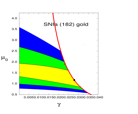
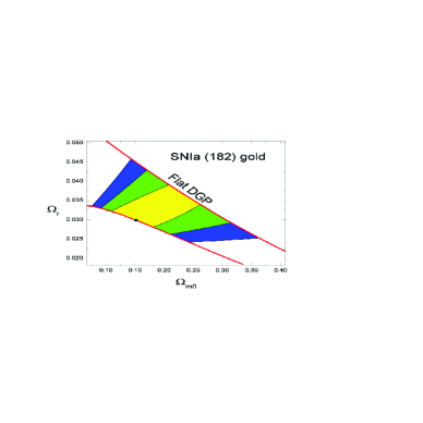
Figure 1: Probability contours at 68.3%, 95.4% and 99.7% confidence levels for joint parameters: (a) ($\gamma$, $\mu_{m0}$)-plane from the gold sample of SNIa data. The point shows the best-fit from the SNIa analysis. The red line corresponds to the limit due to Eq (13). (b) For ($\Omega_{m0}$, $\Omega_{r}$)-plane. The upper boundary corresponds to $\gamma=0$ (pure DGP) and the lower boundary is due to Eq (13).

Table 2:

	$\Omega_{m0}$	$\chi^{2}_{min}$
SNIa	$0.24_{-0.03}^{+0.03}$	159.97
SNIa+LSS	$0.29_{-0.02}^{+0.02}$	162.92
SNIa+LSS+H(z)	$0.27_{-0.02}^{+0.02}$	174.04

An efficient way to reduce the degeneracies of the cosmological parameters is to use the SNIa data in combination with the BAO measurement from SDSS 10 . The acoustic signature in the large scale clustering of galaxies yields additional test of cosmology. Using a large sample of 46748 luminous red galaxies covering 386 square degrees out to a redshif of $z=0.47$ from the SDSS, Einstein et al 10 have found the model independent BAO measurement which is described by the A parameter

$$A \equiv \Omega_{m0}^{1/2}E(z_{\rm BAO})^{-1/3}\left[\frac{1}{z_{\rm BAO}}\int_{0}^{z_{\rm BAO}}\frac{dz^{\prime}}{E(z^{\prime})}\right]^{2/3}$$ (17)

$$= \frac{\mu_{0}^{1/2}E(Z_{\rm BAO})^{-1/3}}{h_{0}}\left[\frac{1}{z_{\rm BAO}}\int_{0}^{z_{\rm BAO}}\frac{dz^{\prime}}{E(z^{\prime})}\right]^{2/3}\leavevmode\nobreak\ .$$

The measurement gives $A=0.469$$(n_{s}/0.98)^{-0.35}\pm 0.017$ at $z_{\rm BAO}=0.35$. The scalar spectral index is taken to be $n_{s}=0.95$ through the three-year WMAP data. In our analysis, we have investigated the joint statistics with the SN Ia data and the BAO measuremen. The results are shown in Fig 2 (a), (b) where we show the contours of 68.3%, 95.4% and 99.7% confidence level for $\mu_{0}$, $\gamma$ and $\Omega_{m0}$, $\Omega_{r}$ respectively. The fitted parameters with the $1\sigma$ errors are shown in Table 1, where $h_{0}$ and $\alpha$ are obtained from $\mu_{0}$ and $\gamma$.

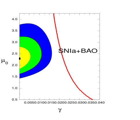
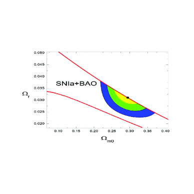
Figure 2: Probability contours at 68.3%, 95.4% and 99.7% confidence levels for joint parameters: (a) ($\gamma$, $\mu_{m0}$)-plane from SNIa+BAO data. The point shows the best-fit. (b) For ($\Omega_{m0}$, $\Omega_{r}$)-plane. The upper line is for the limit $\gamma=0$ while the lower line is due to the limit set by Eq (13).

It is of interest to include the Hubble parameter data to constrain our model. The Hubble parameter depends on the differential age of the universe in terms of the redshift. In contrast to standard candle luminosity distance, the Hubble parameter is not integrated over. It persists fine structure which is highly degenerated in the luminosity distance 14 . Observed values of H(z) 15 can be used to place constraints on the model of the expansion history of the universe by minimizing the quantity

$$\chi^{2}_{H}(\gamma,\mu_{0})=\sum_{i}\frac{\left|H_{obs}(z_{i})-H_{th}(z_{i})\right|^{2}}{\sigma_{i}^{2}}\leavevmode\nobreak\ .$$ (18)

The H(z) test on its own cannot provide tight constrain on the model. It is interesting to combine the H(z) data with other observational data to obtain tighter constraints on the cosmological model. The result on the joint analysis H(z)+SNIa+BAO is shown in Fig 3 (a), (b) respectively. $1\sigma$ range parameters’ spaces are listed in Table 1. It is interesting to notice that errors of model parameters have been significantly reduced.

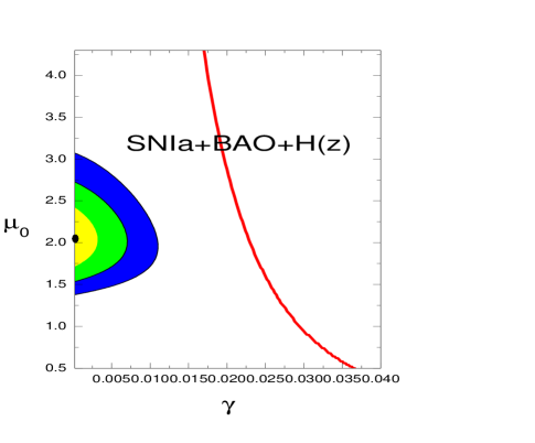
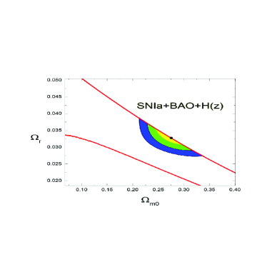
Figure 3: Probability contours at 68.3%, 95.4% and 99.7% confidence levels for joint parameters: (a) ($\gamma$, $\mu_{m0}$)-plane from SNIa+BAO+H(z) data. The point shows the best-fit. (b) For ($\Omega_{m0}$, $\Omega_{r}$)-plane. The upper line is for the limit $\gamma=0$ while the lower line is due to the limit set by Eq (13).

For the sake of comparison, we have also done the fitting to observations by using the pure DGP model where the GB correction is absent. Results are shown in Table 2. Despite the big difference in the single SNIa data fitting, in the combined analysis SNIa+BAO,SNIa+BAO+H(Z), we can see that the GB correction influence the universe evolution, however its effect is very small. In Table 3, we include the fitting results for the pure DGP model obtained in  8 , 11 , 12 . For comparison, we need to notice that $\Omega_{rc}=4\Omega_{r}$. Using our best fit value of $\Omega_{r}$($\Omega_{rc}$), we obtain $r=H_{0}^{-1}\Omega_{rc}^{-1/2}=2.89H_{0}^{-1}$, which obeys the inequality of (10) due to the GB correction.

Table 3:

Model	Test	$\Omega_{m0}$	$\Omega_{r_{c}}$	$\Omega_{K}$	ref
DGP	SNIa	$0.13_{-0.06}^{+0.06}$	$0.14_{-0.03}^{+0.03}$	$0.20_{-0.20}^{+0.20}$	8
DGP	SNIa(new Gold)+CMB+SDSS+LSS	$0.28_{-0.03}^{+0.02}$	$0.13_{-0.01}^{+0.01}$	$-0.002_{-0.053}^{+0.064}$	8
DGP	Gold+SNLS	$0.31_{-0.06}^{+0.07}$	$0.23_{-0.03}^{+0.03}$		11
DGP+GB	SNIa	$0.15_{-0.04}^{+0.11}$	$0.12_{-0.01}^{+0.03}$
DGP+GB	SNIa+LSS	$0.29_{-0.03}^{+0.03}$	$0.13_{-0.01}^{+0.01}$
DGP+GB	SNIa+LSS+H(z)	$0.27_{-0.02}^{+0.03}$	$0.13_{-0.01}^{+0.01}$

If the value of the parameter $\gamma$ is not zero, we can find the maximum redshift at which the universe started its existence in our model. Taking the maximum value of $\gamma$ from Table 1 and using relations (13) and (14) we calculate the $z_{max}$ allowed from observations in our model, which we show in Table 4.

Table 4:

Test	$\gamma$	$\mu_{0}$	$z_{max}$
SNIa	$0.0278$	$1.20_{-0.34}^{+0.70}$	$1.11<z_{max}<1.76$
SNIa+LSS	$0.005$	$2.26_{-0.42}^{+0.55}$	$6.86<z_{max}<8.06$
SNIa+LSS+H(z)	$0.003$	$2.03_{-0.33}^{+0.40}$	$10.76<z_{max}<12.25$

Table IV is actually the result of fitting of our model to the observational data (at late-time with small redshifts). The central zero $\gamma$ corresponds to the infinite $z_{max}$, where the GB effect can be neglected and then the model reduces to the pure DGP. However, what is significant here is that the result is quite sensitive to $\gamma$. Even small nonzero $\gamma$ will cause dramatic change in the evolution of the universe. Table IV takes $\gamma$ just at the edge of $1\sigma$ contour, which illustrates that the effect of GB is significant and quite possible. For the modified DGP model by including the GB correction, it was argued that the combined induced gravity and GB effects make the universe start at a finite maximum density and finite pressure, but with infinite curvature7 . In other words, the universe described in this model does not start at $z=\infty$, but starts at a finite $z$ which is the maximum redshift allowed in the model. $z_{max}$ in Table IV is this maximum redshift when the combined induced gravity and GB effects are taken into account. However, there is a question of the high energy-early-time behaviour of the model. The maximum $z_{max}$ allowed from Table IV is too small to accommodate the conventional CMB formation at high redshifts even if we had the technology to calculate such effects in our model (see cp for such an attempt). Therefore, to go to high redshifts region we have to fine-tune $\gamma$ to very small values, making the contribution of the GB term at late-times negligible.

In summary, in this work we have preformed a parameter estimation of the Induced Gravity model with a higher curvature GB term in the bulk proposed in  7 . We have analyzed data coming from the most recent SN Ia sample, LSS observation and H(z) measurement. The results show that the DGP model with the GB correction is a viable candidate to explain the observed acceleration of our universe. The value of the GB parameter allowed by observation is very small giving only small effects to the corrected DGP model. These correction effects are sensitive to changes of the GB parameter. A nonzero value of $\gamma$ will change significantly the cosmological evolution of our universe. However, to make our model consistent with the conventional CMB formation at high redshifts the GB parameter has to be fine-tuned to very small values.

References

- (1) A. G. Riess et al, Astro. J. 116, 1009 (1998); S. Perlmutter et al, Astrophy. J. 517, 565 (1999).
- (2) I. I. Kogan, S. Mouslopoulos, A. Papazoglou, G. G. Ross and J. Santiago, Nucl. Phys. B 584, 313 (2000) [arXiv:hep-ph/9912552]; I. I. Kogan and G. G. Ross, Phys. Lett. B 485, 255 (2000) [arXiv:hep-th/0003074]; See, e.g., R. Gregory, V. A. Rubakov and S. M. Sibiryakov, Phys. Rev. Lett. 84, 5928 (2000) [arXiv:hep-th/0002072]; I. I. Kogan, [arXiv:astro-ph/0108220]; A. Papazoglou, [arXiv:hep-ph/0112159]; A. Padilla, Class. Quant. Grav. 22, 681 (2005) [arXiv:hep-th/0406157]; A. Padilla, Class. Quant. Grav. 22, 1087 (2005) [arXiv:hep-th/0410033].
- (3) G. R. Dvali, G. Gabadadze and M. Porrati, Phys. Lett. B 485, 208 (2000) [arXiv:hep-th/0005016]. G. R. Dvali, G. Gabadadze and M. Porrati, Phys. Lett. B 485, 208 (2000) [arXiv:hep-th/0005016]; G. R. Dvali and G. Gabadadze, Phys. Rev. D 63, 065007 (2001) [arXiv:hep-th/0008054]; C. Deffayet, Phys. Lett. B 502, 199 (2001) [arXiv:hep-th/0010186]; C. Deffayet, G. R. Dvali and G. Gabadadze, Phys. Rev. D 65, 044023 (2002) [arXiv:astro-ph/0105068]; A. Lue, [arXiv:astro-ph/0510068].
- (4) C. Charmousis, R. Gregory, N. Kaloper and A. Padilla, JHEP 0610, 066 (2006) [arXiv:hep-th/0604086]. A. Padilla, [arXiv:hep-th/0610093]. K. Koyama, Phys. Rev. D 72, 123511 (2005) [arXiv:hep-th/0503191]; D. Gorbunov, K. Koyama and S. Sibiryakov, Phys. Rev. D 73, 044016 (2006) [arXiv:hep-th/0512097].
- (5) V. A. Rubakov, [arXiv:hep-th/0303125]. M. A. Luty, M. Porrati and R. Rattazzi, JHEP 0309, 029 (2003) [arXiv:hep-th/0303116]. S. L. Dubovsky and M. V. Libanov, JHEP 0311, 038 (2003) [arXiv:hep-th/0309131]. M. N. Smolyakov, Phys. Rev. D 72, 084010 (2005) [arXiv:hep-th/0506020].
- (6) See, e.g., C. Charmousis and J. F. Dufaux, Class. Quant. Grav. 19, 4671 (2002) [arXiv:hep-th/0202107]; S. Nojiri, S. D. Odintsov and S. Ogushi, Int. J. Mod. Phys. A 17, 4809 (2002) [arXiv:hep-th/0205187]; S. C. Davis, Phys. Rev. D 67, 024030 (2003) [arXiv:hep-th/0208205]; J. E. Lidsey and N. J. Nunes, Phys. Rev. D 67, 103510 (2003) [arXiv:astro-ph/0303168]; K. i. Maeda and T. Torii, Phys. Rev. D 69, 024002 (2004) [arXiv:hep-th/0309152]; J. F. Dufaux, J. E. Lidsey, R. Maartens and M. Sami, Phys. Rev. D 70, 083525 (2004) [arXiv:hep-th/0404161]; T. G. Rizzo, JHEP 0501, 028 (2005) [arXiv:hep-ph/0412087].
- (7) N. E. Mavromatos and E. Papantonopoulos, [arXiv:hep-th/0503243].
- (8) R. A. Brown, R. Maartens, E. Papantonopoulos and V. Zamarias, JCAP 0511, 008 (2005) [arXiv:gr-qc/0508116].
- (9) G. Kofinas, R. Maartens and E. Papantonopoulos, JHEP 0310, 066 (2003) [arXiv:hep-th/0307138].
- (10) T. Koivisto, D. F. Mota, Phys.Lett.B644, 104 (2007); Phys.Rev.D75, 023518,(2007).
- (11) R. Maartens and E. Majerotto, Phys. Rev. D 74, 023004 (2006) [arXiv:astro-ph/0603353]; M.C. Bento, O. Bertolami, M.J. Reboucas, N.M.C. Santos, Phys.Rev. D73 (2006) 103521.
- (12) S. Rydbeck, M. Fairbairn and A. Goobar, JCAP 0705, 003 (2007) [arXiv:astro-ph/0701495].
- (13) M. S. Movahed, M. Farhang and S. Rahvar, [arXiv:astro-ph/0701339].
- (14) Z. K. Guo, Z. H. Zhu, J. S. Alcaniz and Y. Z. Zhang, Astrophys. J. 646, 1 (2006) [arXiv:astro-ph/0603632].
- (15) N. Pires, Z. H. Zhu and J. S. Alcaniz, Phys. Rev. D 73, 123530 (2006) [arXiv:astro-ph/0606689].
- (16) A. Sheykhi, B. Wang and N. Riazi, Phys. Rev. D 75, 123513 (2007).
- (17) R.G.Cai, H.S.Zhang and A.Wang, Commun. Theor. Phys. 44, 948 (2005).
- (18) K. Koyama and R. Maartens, JCAP 0601, 016 (2006).
- (19) M.C. Bento, O. Bertolami, M.J. Rebou?as, N.M.C. Santos, Phys.Rev. D73 (2006) 103521.
- (20) A. G. Riess et al., [arXiv:astro-ph/0611572].
- (21) D. J. Eisenstein et al. [SDSS Collaboration], Astrophys. J. 633, 560 (2005) [arXiv:astro-ph/0501171].
- (22) H. Wei and S. N. Zhang, Phys. Lett. B 644, 7 (2007) [arXiv:astro-ph/0609597]; P. Wu and H. W. Yu, Phys. Lett. B 644, 16 (2007) [arXiv:gr-qc/0612055]; P. X. Wu and H. W. Yu, JCAP 0703, 015 (2007) [arXiv:astro-ph/0701446]; L. I. Xu, C. W. Zhang, B. R. Chang and H. Y. Liu, [arXiv:astro-ph/0701519]; A. Kurek and M. Szydlowski, [arXiv:astro-ph/0702484]; H. Zhang and Z. H. Zhu, [arXiv:astro-ph/0703245].
- (23) J. Simon, L. Verde and R. Jimenez, Phys. Rev. D 71, 123001 (2005) [arXiv:astro-ph/0412269].
- (24) S. Tsujikawa, M. Sami and R. Maartens, Phys. Rev. D 70, 063525 (2004).