Also at ]Center for Nonlinear Phenomena and Complex Systems, Universite Libre de Bruxelles, Code Postal 231, Campus Plaine, B-1050 Brussels, Belgium.
Entropy fluctuation theorems in driven open systems: application to electron counting statistics
Abstract
The total entropy production generated by the dynamics of an externally driven systems exchanging energy and matter with multiple reservoirs and described by a master equation is expressed as the sum of three contributions, each corresponding to a distinct mechanism for bringing the system out of equilibrium: nonequilibrium initial conditions, external driving, and breaking of detailed balance. We derive three integral fluctuation theorems (FTs) for these contributions and show that they lead to the following universal inequality: an arbitrary nonequilibrium transformation always produces a change in the total entropy production greater or equal than the one produced if the transformation is done very slowly (adiabatically). Previously derived fluctuation theorems can be recovered as special cases. We show how these FTs can be experimentally tested by performing the counting statistics of the electrons crossing a single level quantum dot coupled to two reservoirs with externally varying chemical potentials. The entropy probability distributions are simulated for driving protocols ranging from the adiabatic to the sudden switching limit.
I Introduction
In statistical mechanics, thermodynamic laws are recovered at the level of ensemble averages.
The past decade has brought new insights into nonequilibrium statistical mechanics due to
the discovery of various types of fluctuation relations valid arbitrarily far from equilibrium
Evans1 ; Gallavotti ; Evans2 ; Jarzynski1 ; Kurchan ; Lebowitz ; Evans3 ; Crooks99 ; Crooks00 ; Hatano99 ; Hatano01 ; Gaspard1 ; GaspardAndrieux ; Seifert1 ; Seifert2 ; Chernyak ; Broeck .
These relations identify, at the level of the single realization of a statistical ensemble,
the ”trajectory entropy” which upon ensemble averaging reproduce the thermodynamic entropy.
They therefore quantify the statistical significance of nonthermodynamic behaviors
which can become significant in small systems Bustamante0 ; GaspardAndrieux2 .
Various experimental verifications of these FTs have been reported
Bustamante1 ; Bustamante2 ; Bustamante3 ; Douarche ; Evans ; Wrachtrup1 ; Wrachtrup2 .
In this paper, we consider an open system, described by a master
equation (ME), exchanging matter and energy with multiple reservoirs.
The system can be externally driven by varying its energies or the different
temperature or chemical potentials of the reservoirs.
There are three mechanisms for bringing such a system out of equilibrium:
preparing it in a nonequilibrium state, externally driving it,
or putting it in contact with multiple reservoirs at different temperatures
or chemical potentials thus breaking the detailed balance condition (DBC).
We show that each of these mechanism makes a distinct contribution to the total
entropy production (EP) generated by the nonequilibrium dynamics of the system.
The two first contributions are nonzero only if the system is not in its steady
state and are therefore called nonadiabatic.
The third contribution is equal to the EP for slow transformation during which
the system remains in a steady-state and is therefore called adiabatic.
We derive three FTs, for the total EP and its nonadiabatic and adiabatic contribution
and show that they lead to exact inequalities valid arbitrary far from equilibrium.
Previously derived FTs are recovered by considering
specific types of nonequilibrium transformations.
Steady state FTs Lebowitz ; Gaspard1 ; GaspardAndrieux are obtained for
systems maintained in a nonequilibrium steady state (NESS) between reservoirs with
different thermodynamic properties.
The Jarzynski or Crooks type FTs Jarzynski1 ; Crooks99 ; Crooks00
are derived for systems initially at equilibrium with a single reservoir
which are externally driven out of equilibrium by an external force.
The Hatano-Sasa FT Hatano99 ; Hatano01 is recovered for externally driven
systems initially in a NESS with multiple reservoirs.
To calculate the statistical properties of the various contributions to the
total EP and to demonstrate the FTs, we extend the generating
function (GF) method Lebowitz to driven open systems.
Apart from providing clear proofs of the various FTs, this method is useful for simulations
because it does not require to explicitly generate the stochastic trajectories.
Some additional insight is provided by using an alternative derivation
of the FTs similar to the Crooks derivation Crooks99 ; Crooks00 ,
where the total EP and its nonadiabatic part can be identified in terms of
forward-backward trajectory probabilities.
By doing so, we connect the trajectory approach previously
used for driven closed systems Seifert1 ; Crooks99 ; Crooks00 with the
GF approach used for steady state systems Lebowitz ; Gaspard1 .
We propose to experimentally test these new FTs in a driven single orbital quantum dot
where the various entropy probability distributions can be measured by the
full electron counting statistics which keeps track of the four possible types of
electron transfer (in and out of the dot through either lead).
Such measurements of the bidirectional counting
statistics have become feasible recently Hirayama .
We calculate the entropy probability distributions, analyze
their behavior as the driving is varied between the sudden and the
adiabatic limits, and verify the validity of the FTs.
In section II we present our stochastic model and in section III we describe the various contributions to the total EP generated during a nonequilibrium transformation and the inequalities that these contributions satisfy. In section IV, we define the various trajectory entropies which upon ensemble averaging give the various contributions to the EP. We then present the GF formalism used to calculate the statistical properties of these trajectory entropies. In section V, we derive the various FTs and the implied inequalities. Alternative derivations of FTs in terms of forward-backward trajectories are given in appendix A. By considering specific nonequilibrium transformations, we recover most of the previously derived FTs. Finally in section VI, we apply our results to the full counting statistics of electrons in a driven quantum dot. Conclusions are drawn in section VII.
II The master equation
We consider an externally driven open system exchanging particles and energy with multiple reservoirs. Each state of the system has a given energy and particles. The total number of states is finite and equal to . The probability to find the system in a state at time is denoted by . The evolution of this probability is described by the ME
| (1) |
where the rate matrix satisfies
| (2) |
We assume that if a transition from to can occur,
the reversed transition from to can also occur.
Various parameters, such as the energies of the
system or the chemical potential and the
temperature of the reservoir can be
varied in time externally according to a known protocol.
This is described by the dependence of
the rate matrix on several time-dependent parameters .
If the transition rates are kept constant, the system will eventually
reach the unique steady state solution
which satisfies note1 .
The transition rates will be expressed as sums of contributions from different reservoirs
| (3) |
each satisfying
| (4) | |||||
If all reservoirs have the same thermodynamic properties (temperature and chemical potential ), the steady state distribution coincide with the equilibrium distribution which satisfies the detailed balanced condition (DBC)
| (5) |
As a consequence of (4) and (5), the equilibrium distribution then assumes the grand canonical form
| (6) |
where is the grand canonical partition function. However, in the general case where the reservoirs have different and , the DBC does not hold and is a NESS.
III The entropies
The Gibbs entropy of the system is a state function defined as
| (7) |
Using (1) and (2), the system EP reads
| (8) | |||||
This can be partitioned as Prigogine ; GrootMazur ; Schnakenberg ; Gaspard1 ; Seifert1
| (9) |
with the total EP
and the reservoir EP (also called medium entropy or entropy flow)
| (11) |
We note that
follows from if
and for (if the log in zero),
by using the fact that
and .
is the contribution to coming from the
changes in the system probability distribution and is
the contribution coming from matter and energy exchange processes
between the system and its reservoirs.
We further separate the reservoir EP into two components Hatano01 ; Seifert2
| (12) |
with the excess EP
and the adiabatic EP (also called housekeeping entropy Hatano01 ; Seifert2 )
The positivity of (III) follows from the same reason as (III).
If a transformation is done very slowly, the system remains at all
times in the steady state distribution .
Such a transformation is called adiabatic.
We then have and .
We also notice that when the DBC is satisfied.
We next define the state function quantity
| (15) |
which is obviously zero when the system is at steady state. When considering a transformation between steady states, . We call the boundary EP (the terminology will be explain shortly) and separate it in two parts
| (16) |
where the nonadiabatic EP is
and the driving EP is
| (18) |
with
| (19) |
The positivity of (III) is again shown in the same way as for (III) and (III). If no external driving acts on the system, is time independent and from (18), . For an adiabatic transformations, since , from (15) and (III), we see that as well as . From (16), this also means that . Therefore, only for nonadiabatic driving. Using (III) with (8) and (III), we find
| (20) |
It is clear from the last equality why we call the nonadiabatic EP. The inequality which follows from the first line is a generalization of the ”second law of steady state thermodynamics” Oono ; HTasaki ; Hatano01 derived for transitions between steady states.
We next summarize our results
| (21) | |||||
| (22) | |||||
| (23) |
The total EP is always positive and can be separated into two positive contributions, adiabatic (which are nonzero only when the DBC is violated) and nonadiabatic effects. The latter can be due to a nonadiabatic external driving acting on the system or to the fact that one considers transformation during which the system is initially or finally not in a steady state. We therefore have a minimum EP principle stating that the total EP for arbitrary nonequilibrium transformations takes its minimal value if the transformation is done adiabatically (very slowly). The equality sign in (21) is satisfied for adiabatic transformations which occur at equilibrium. The equality sign in (22) holds for adiabatic transformations. The equality sign in (23) only occurs when the DBC is satisfied.
IV Trajectory entropies
The evolution described by the ME can be represented by
an ensemble of stochastic trajectories involving instantaneous jumps
between states. This will allow us to define fluctuating (trajectory) entropies.
IV.1 Definitions
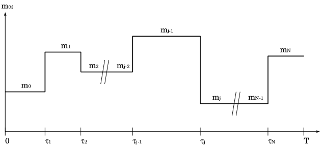
We denote a trajectory taken by the system between and by
.
At the system is in , and stays there until it jumps at to ,
etc., jumps at from to and stays in until
[see Fig. 1]. is the total number of jumps during this trajectory.
We next introduce various type of ’trajectory entropy production’ (TEP).
We will see at the end of this section that
when ensemble averaged, these correspond to the various
EP defined in section III.
The trajectory Gibbs entropy is defined as
| (24) |
where represents the value of along the trajectory . The system TEP is given by
| (25) |
The first term represents the smooth changes of along the horizontal
segments of the trajectory on Fig. 1 during which the system is in a well
defined state. These changes are only due to the time dependence of the probability
to be on a given state.
The notation means that the in the expression
changes depending on which horizontal segment along the trajectory one considers.
The second term represents the discrete changes of
along the vertical segments of the trajectory.
These changes are singular and only due to the change in the system state.
Separating the trajectory system TEP similarly as the system
EP in section III, we get
| (26) |
where the total TEP is
and the reservoir TEP
| (28) |
We further separate the reservoir TEP into
| (29) |
with the adiabatic TEP
| (30) |
and the excess TEP
| (31) |
The nonadiabatic TEP
is made of the sum of two terms
| (33) |
the boundary TEP
and the driving TEP
As in section III, since
| (35) |
we get
| (36) |
We generically denote these TEP by . The change of along a trajectory of length is given by
| (37) |
Notice that and are state function TEP
| (38) |
where , and
The other TEP are path functions.
IV.2 Deriving trajectory entropies from measured currents
Using (4), the reservoir TEP can be expressed as
| (40) | |||
where the heat current between the reservoir and the system is
| (41) |
and the matter current between the reservoir and the system
| (42) |
The currents are positive if the system energy (matter) increases.
is a Dirac distribution centered
at time only if the transition is due to the reservoir .
Otherwise it is zero.
We thus confirm that the reservoir EP is the entropy associated to
system-reservoir exchange processes.
We assume that the parametric time dependence of the energies, temperatures and chemical potentials is known. Except in degenerate cases for which two different transitions between states have the same energy difference and number of particle difference, the trajectory of the system can be uniquely determined by measuring the heat and matter currents between the system and the reservoirs. The system steady state probability distribution can be calculated by recording the steady state currents for sufficiently long times for different values of the energies, temperatures or chemical potentials. The driven system probability distribution can in principle be calculated by reproducing the measurement of the currents multiple times. All trajectory entropies containing the logarithm of the transition rates can be expressed in term of a combination of the reservoir EP (directly measurable via current) and other trajectory entropies which can be expressed in term of the system probability distribution (actual or steady state). Therefore, provided the current measurements can be repeated often enough to get a good statistics, all the trajectory entropies are in principle measurable.
IV.3 Statistical properties using generating functions
The GF formalism allows to compute the probability distributions and all statistical
properties of the TEP without having to generate the trajectories themselves.
It further provides a direct means for proving the FTs.
The GF associated with the changes of along a trajectory is given by
| (43) |
where denotes an average over all possible trajectories. The probability that the system follows a trajectory with the constraint at time , can be obtained from the GF using
By inverting (IV.3), we get
| (45) |
The moments of the distribution are given by derivatives of the GF
| (46) |
In order to compute the GF, we recast it in the form
| (47) |
where
| (48) |
is the product of the probability to find the system in state at time
multiplied by the expectation value of
conditional on the system being in state at time .
Since for a trajectory of length , we have
. We also have and .
The time derivative of (47) gives
| (49) |
where depends on the TEP of interest. Below, we will derive equations of motion for the ’s associated to the various TEP.
IV.3.1 State function trajectory entropy production
IV.3.2 Excess trajectory entropy production
acquires an amount each time a transition from a state to occurs and it remains constant along a given state of the system. This means that
which using (48) can be rewritten
| (52) |
IV.3.3 Reservoir trajectory entropy production and currents
Each time a transition along the system trajectory occurs, acquires an amount . Similarly to the excess entropy, we get
| (53) |
This equation has been used in the study of steady
state FTs Lebowitz ; Gaspard1 ; GaspardAndrieux1 .
In (40), we expressed the reservoir TEP in terms of currents. The time integrated individual currents give the heat and matter transfer between the reservoir and the system and . Their statistics can be calculated using
| (54) | |||||
where is a vector who’s elements are the different ’s and ’s. The GF calculated from (54) is therefore associated with the join probability distribution for having a certain heat and matter transfer with each reservoir.
IV.3.4 Adiabatic trajectory entropy production
Each time a transition along the system trajectory occurs, acquires an amount . We therefore get
IV.3.5 Total trajectory entropy production
Each time a transition along the system trajectory occurs, acquires an amount . In addition it also changes by an amount during an infinitesimally small time on a given state of the system. Combining the two, we have
IV.3.6 Non-adiabatic trajectory entropy production
Like the total TEP, acquires an amount each time a transition from a states to occurs, and also changes by an amount during an infinitesimally small time on a given state . This gives
IV.3.7 Driving trajectory entropy production
Since exclusively accumulates along the segments of the system trajectory, we get
It follows from (46) that the average change of a TEP is obtained from its GF by differentiation with respect to at . By differentiating the GF evolution equations of this section one recover the evolution equation for the EPs of section III. The EPs are therefore the ensemble average of the TEPs introduced in this section and .
V Fluctuation theorems
V.1 General integral fluctuation theorems
We can easily verify that is the solution of the evolution equations (IV.3.5) and (IV.3.6). It immediately follows from probability conservation and (49) that . Summing both side of (IV.3.4) over , we also verify that . Because , where . Therefore, we find that . Using (43), this results in the three FTs
| (59) | |||
| (60) | |||
| (61) |
These FTs hold irrespective of the initial condition and the type of driving.
Using Jensen’s inequality ,
they imply the inequalities (21)-(23).
Eq. (59) is the generalization to open systems of
the integral FT for the TEP obtained earlier
for closed systems Seifert1 .
The TEP (IV.1) needs to specify which
reservoir is responsible for the transitions occurring along the
trajectory (by labeling the rates with reservoir index).
This point, made earlier for open system at steady state Gaspard1 ,
is generalized here for driven systems with an arbitrary initial condition.
Eq. (60) will be shown in next section to reduce to the integral
Hatano-Sasa FT Hatano01 for systems initially in a steady state.
Eq. (61) generalizes the integral FT for the adiabatic entropy
Seifert2 previously derived for closed system initially in a steady state.
V.2 Transitions between steady states
We consider a system initially (t=0) at steady state and subjected to an external driving force between and . For , the system remains in the steady state corresponding to . The time protocol of during the driving is arbitrary. If is the characteristic transient time needed for the system to reach a steady state from an arbitrary distribution, for , the system is in the new steady state corresponding to . The system is measured between and .
V.2.1 Fluctuation theorem for the reservoir entropy production
We restrict our analysis to cases where the system is at steady state
at and the driving starts at least a time after the
measurement started: .
We use the braket notation where is the probability vector
with components and denotes the rate matrix.
denotes a vector with all components equal to one.
The ME (1) now reads
| (62) |
The generating function for the reservoir EP (53) for evolves according to the adjoint equation of (62)
| (63) |
The initial condition of (62) and (63) is . The formal solution of (63) for before the driving starts reads
| (64) |
We now insert a closure relation in term of right and left eigenvectors of the adjoint rate matrix between the evolution operator and the initial condition. Because the rate matrix and its adjoint have the same eigenvalues (all negative and one zero), for , only the right and left eigenvector associated with the zero eigenvalue survive. Since the right [left] eigenvector of is [], we get for
| (65) |
For longer times, even when the system starts to be driven, remains invariant under the time evolution operator as can be seen using (2) in (63). We get
| (66) |
where is the total number of states. This implies the following integral FT for the reservoir TEP
| (67) |
The equality on the l.h.s (r.h.s) is satisfied if (). Jensen’s inequality implies . Note that since is a state function, it is easily verified that
| (68) |
V.2.2 The Hatano-Sasa fluctuation theorem
We assume that the driving starts at the same time or later as the measurement ().
We define .
We have pointed out at the end of section III that for transitions
between steady states , so that
| (69) |
We used the fact that starts (stops) evolving at (). The same is true at the trajectory level, since from (IV.1) we have and therefore
| (70) |
where
The integrand in the third line contributes only during the time intervals between jumps provided the driving is changing. Therefore if without loss of generality we choose the measurement time such that (if one can redefine as equal to ), . This means that for a transition between steady states, the FT (60) reduces to the Hatano-Sasa FT Hatano01
| (72) |
Alternatively, (72) can be proved from (IV.3.7) by showing that when , is solution of (IV.3.7).
The FT (72) holds for an arbitrary driving protocol. Let us consider the two extremes. For an adiabatic (infinitely slow) driving, the inequality in (69) becomes an equality. In the other extreme of a sudden driving, where and ,
| (73) |
becomes a state function and its average takes the simple form
| (74) |
Using (35) with (70), and since
| (75) |
we find that
| (76) |
also becomes a state function and its average becomes
| (77) | |||||
V.3 Transitions between equilibrium states
For a system coupled to a single reservoir (or multiple reservoirs with identical thermodynamical properties), the DBC (5) is satisfied. A non-driven system in an arbitrary state will reach after some transient time the equilibrium grand canonical distribution (6). We again choose and . From the TEP of section IV, we find in this case
| (78) | |||||
The two FT (59) and (60) become identical and the FT (61) becomes trivial. Using (6), we also find that Eq. (19) becomes
| (79) |
where is
the thermodynamic grand canonical potential.
We next consider transitions between equilibrium states,
so that the procedure is the same as in V.2.2 but with
the DBC (5) now satisfied.
We therefore have .
The driving implies externally modulating the system energies, the
chemical potential or the temperature of the reservoir.
When driving the system energy, using (V.2.2) and (79), we find
| (80) |
where the work is given by and . Both FT, (59) and (60), lead to the same Jarzynski relation Jarzynski1
| (81) |
When driving the reservoir chemical potential, Eq. (V.2.2) and (79) give
| (82) |
where and . Both FT, (59) and (60), now lead to
| (83) |
The case where reservoir temperature is driven can be calculated similarly.
V.4 No driving: steady state fluctuation theorem
In a NESS, the relations of section IV give
| (84) | |||||
Furthermore, since , we get
| (85) |
We shall rewrite the GF evolution equation for the reservoir TEP (53) in the bracket notation
| (86) |
so that
| (87) |
where is a vector with all elements equal to one. Since from (53) the generator has the property , its eigenvalues have the symmetry . Furthermore, since is a positive matrix, the Frobenious-Perron theorem Stirzaker ; Norris ; Kampen ensures that all eigenvalues are negative or zero and that the left and the right eigenvectors, and , associated with the largest eigenvalue exist. Adopting the normalization , we find for long times
| (88) |
and that
This means that the cumulant generating function
| (90) |
satisfies the symmetry
| (91) |
Using the theory of large fluctuations this symmetry implies the detailed steady state FT Lebowitz ; Gaspard1
| (92) |
where is the probability for a trajectory
of the system to produce a reservoir TEP equal to .
grows in average with time because it
depends on the number of jumps along the trajectory.
However, is bounded.
The FT (92) can therefore be viewed as a consequence
of the detailed FT for derived in (119).
The long time limit is needed in order to neglect the contribution
from to .
The FT (67) remains valid at steady state.
FTs for currents can also be derived
GaspardAndrieux2 ; GaspardAndrieux1 ; EspositoHarbola2 .
VI Entropy fluctuations for electron transport trough a single level quantum dot
We have seen in section IV.2 that the various entropies can be calculated
by measuring the different currents between the system and the reservoirs.
The counting statistics of electrons through quantum dots has recently raised
considerable theoretical
Levitov ; Rammer ; Nazarov ; Utsumi ; EspositoHarbola2 as
well as experimental Lu ; Fujisawa ; Bylander ; Gustavsson ; Hirayama interest.
The single electrons entering and exiting a quantum dot connected to two leads can be measured.
One can therefore calculate all currents, deduce the system trajectories
and calculate the various trajectory entropies presented earlier.
We will analyze the probability distribution for the various trajectory entropies in a single level quantum dot of energy connected to two leads with different chemical potentials , where . We neglect spin so that the dot can either be empty or filled . The ME is of the form (1) Nazarov ; Beenakker ; Bonet ; Elste ; Datta1 ; Datta2 ; EspositoHarbola1
| (99) |
where
| (100) |
The coefficients characterize the coupling between the dot and the lead with Fermi distribution . If , . By renormalizing energies by , all parameters of our model become dimensionless. The steady state distribution of the system is
| (101) |
and the steady state currents are given by
| (102) |
We switch the chemical potential of the left lead using the protocol
| (103) |
while holding the right lead chemical potential fixed .
We can therefore calculate all the trajectory entropies’ probability
distributions using the GF method described in section IV.3.
We solve numerically the evolution equations for the ’s
associated with the different entropies for different values of
with the initial condition .
After calculating the ’s using (47), the probability
distribution is obtained by a numerical inverse Fourier transform (IV.3).
In all calculations we used , , and .
We start by analyzing the different contributions to the EP as defined in section III
for the protocol shown in Fig. (2)a.
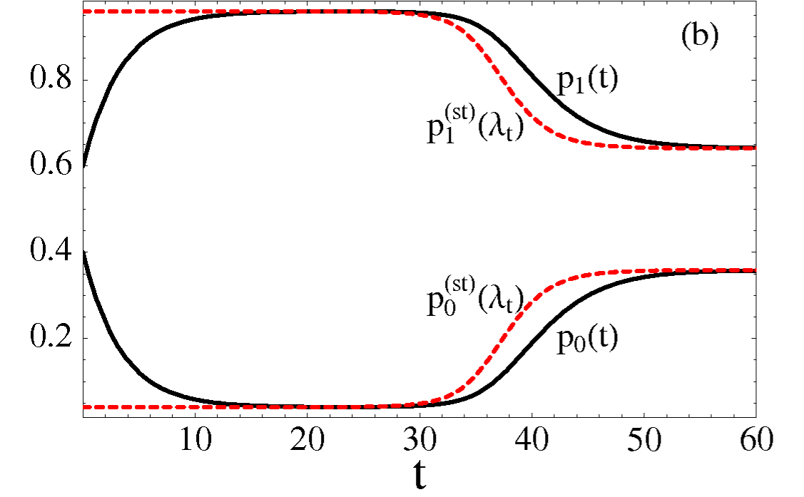
The system is initially in a nonequilibrium distribution different from the steady state.
The solution of the ME (99) as well as its steady state solution are displayed in Fig. 2b.
Between and , is essentially constant and the system undergoes an
exponential relaxation to the steady state.
Between and , changes from to fast enough for the system
distribution to start differing again from the instantaneous steady state distribution (adiabatic solution).
After , remains constant and the system again undergoes a transient
relaxation to the new steady state corresponding to .
Fig. 2c shows the time dependent EP and its adiabatic
and nonadiabatic contribution .
As predicted, these three quantities are always positive [see (21)-(23)].
We also demonstrate that only contributes when nonadiabatic effects are significant
i.e. when the actual probability distribution is different from the steady state one
[].
only once at , when
and the DBC is satisfied. Otherwise the DBC is broken and .
In Fig. 2d, we present the two contributions to the nonadiabatic EP ,
the driving EP and the boundary EP [see (22)].
The driving EP only contributes when changes in time.
One can also guess that due to the fact that the
change of boundary EP during an interval between two steady state is zero.
because the system is initially not in a steady state.
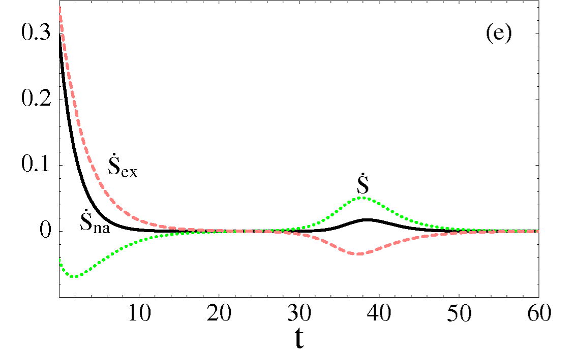
Fig. 2e shows the alternative partitioning of the nonadiabatic EP into
the system EP and the excess EP [see (20)].
Finally the splitting of the total EP in the reservoir EP and the system EP [see (9)]
is shown in Fig. 2f.
We see that at steady state so that .
We next study the statistical properties of the different TEP for transitions between steady states.
The probability distributions are obtained using the GF method presented in section IV.3.
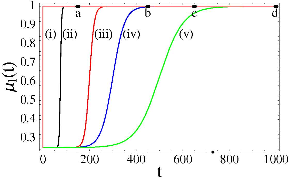
The five driving protocols used to change from to
are presented in Fig. 3.
They range from sudden switch in (i) to slow (adiabatic) switch in (v).
The system is always initially in the steady state corresponding to .
We will consider measurements which end when the system reaches its new steady state at .
Different measurement times are represented by a,b,c,d.
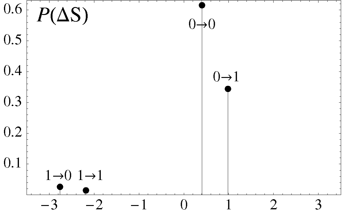
In Fig. 4, we display .
Since is a state function, is the same for the various protocol.
Because we consider a two level system, can only take four possible values which
correspond to the four possible change in the system state between its initial and final condition.
The transitions and are much more probable because the probability to
initially find the system in the empty state is much higher ()
than finding it in the filled state ().
The transition is more probable than because the system
has a final probability to be in its empty state and to be in its filled state.
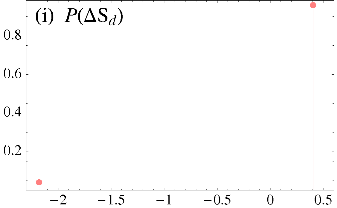
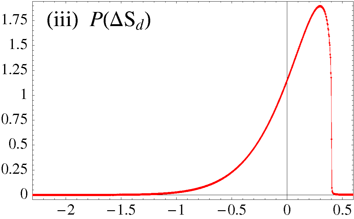
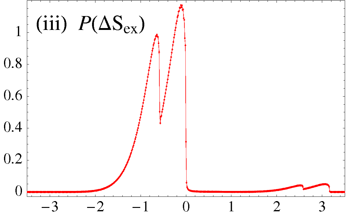
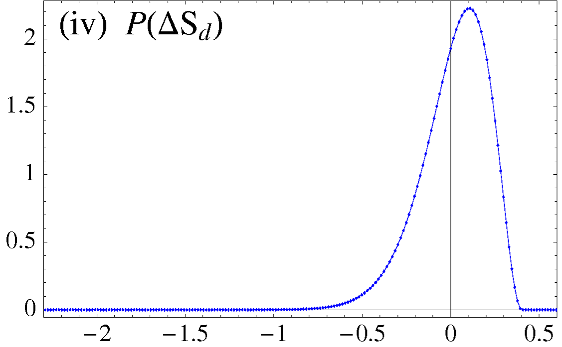
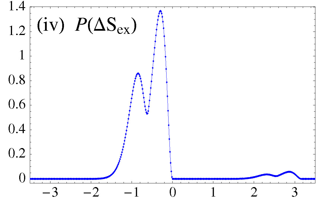
In the left column of Fig. 5, we depict .
Here so that [see (16)].
All curves (i)-(v) satisfy the FT (60).
For the sudden switch (i), becomes a state function
which only depends on the initial state of the system [see (73)].
can therefore take two possible values corresponding to the
empty or filled orbital with a respective probability or .
When the driving speed slows down in (ii) the peaks are broadened.
In the adiabatic limit (V), becomes a broad distribution with zero average.
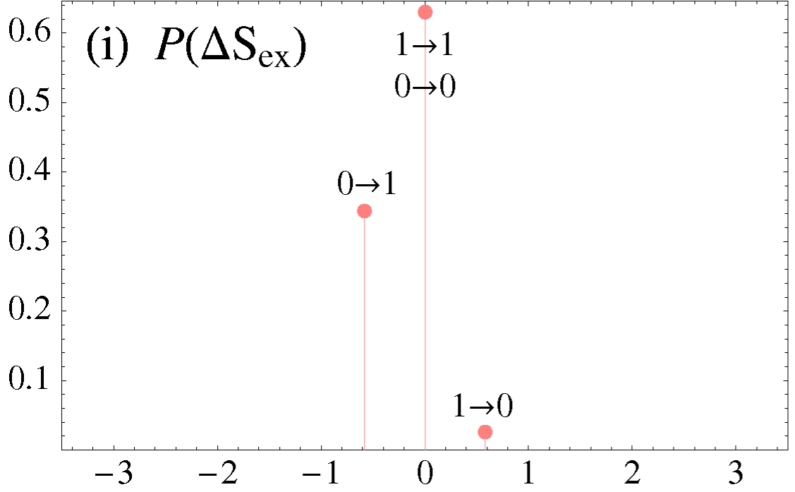
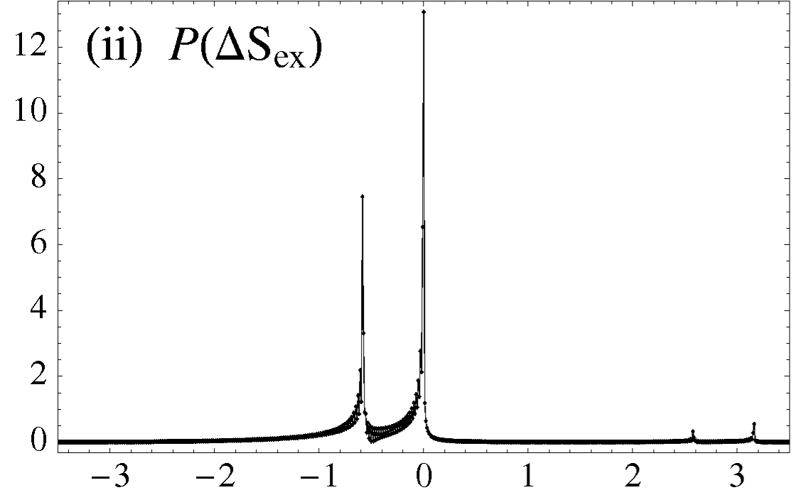
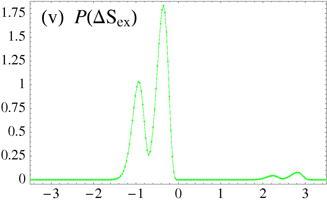
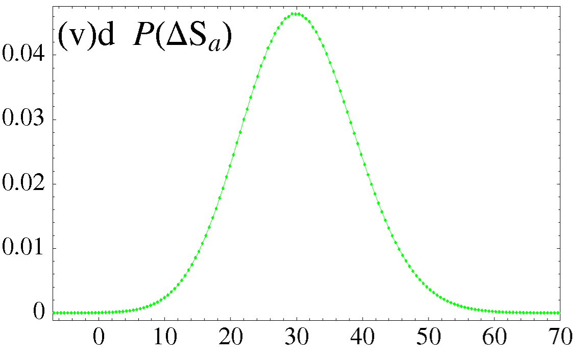
In the right column of Fig. 5, we depict .
For sudden switch (i), turn to a state function which only
depends on the final steady state distribution [see (76)].
It is clear from (76) that the transitions and leads to
and and to the same with opposite sign.
The probabilities to observe these transitions follow from the fact that
the system is initially more likely to be in (prob ) than in .
The probability for the final state () is ().
Therefore the most likely transition is followed from .
As the driving speed slows down like in (ii), the peaks get broadened.
Since [see (20)] and since
in the adiabatic switch limit (v) is centered around zero,
(v) has the same peak structure as
[see Fig. 4], but broadened by .
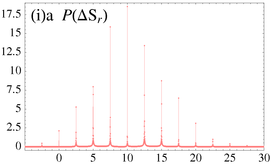
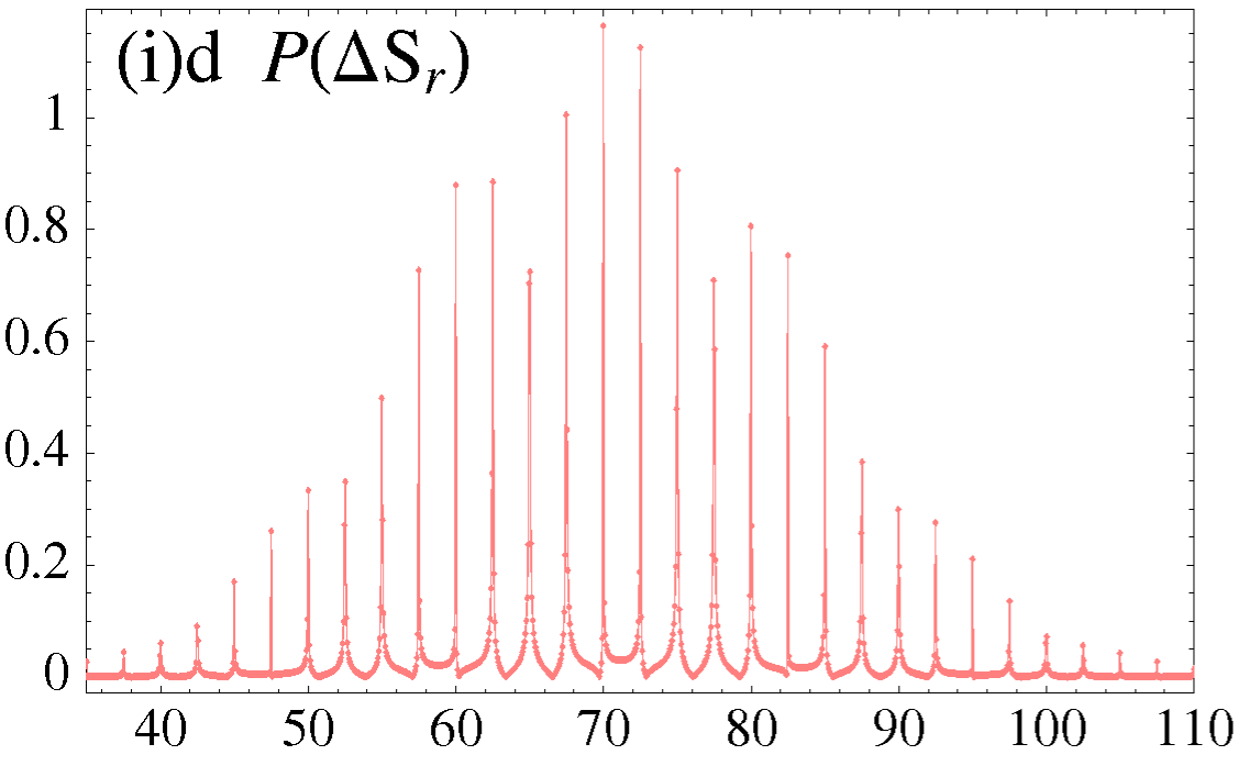
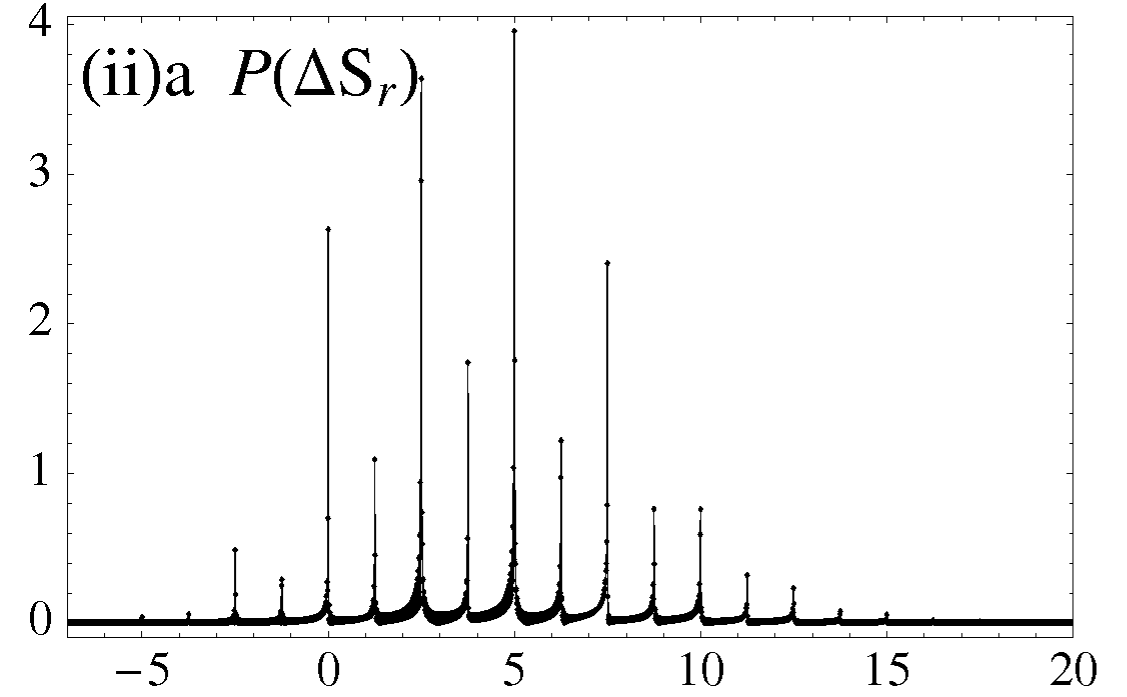
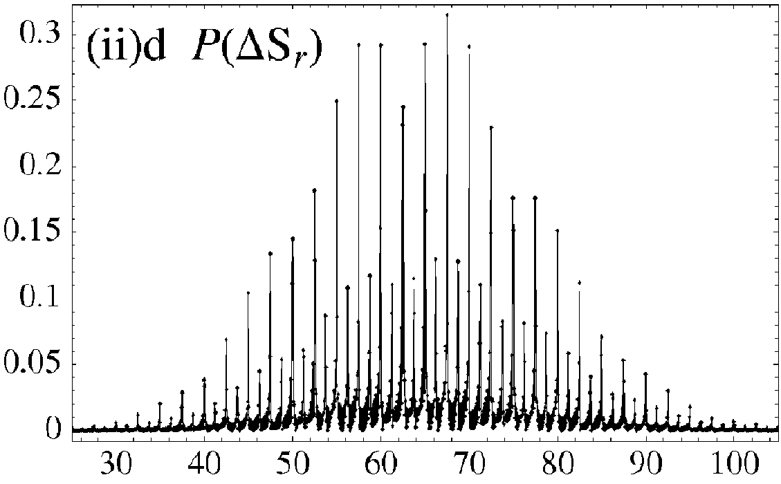
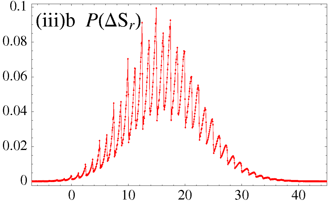
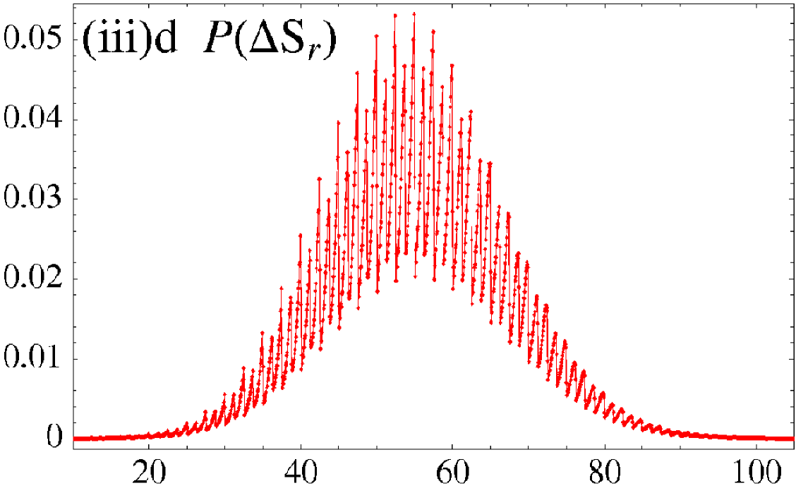
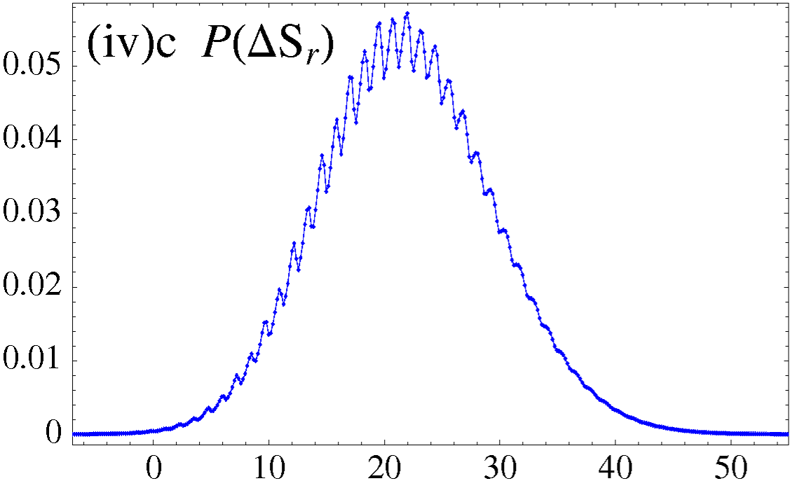
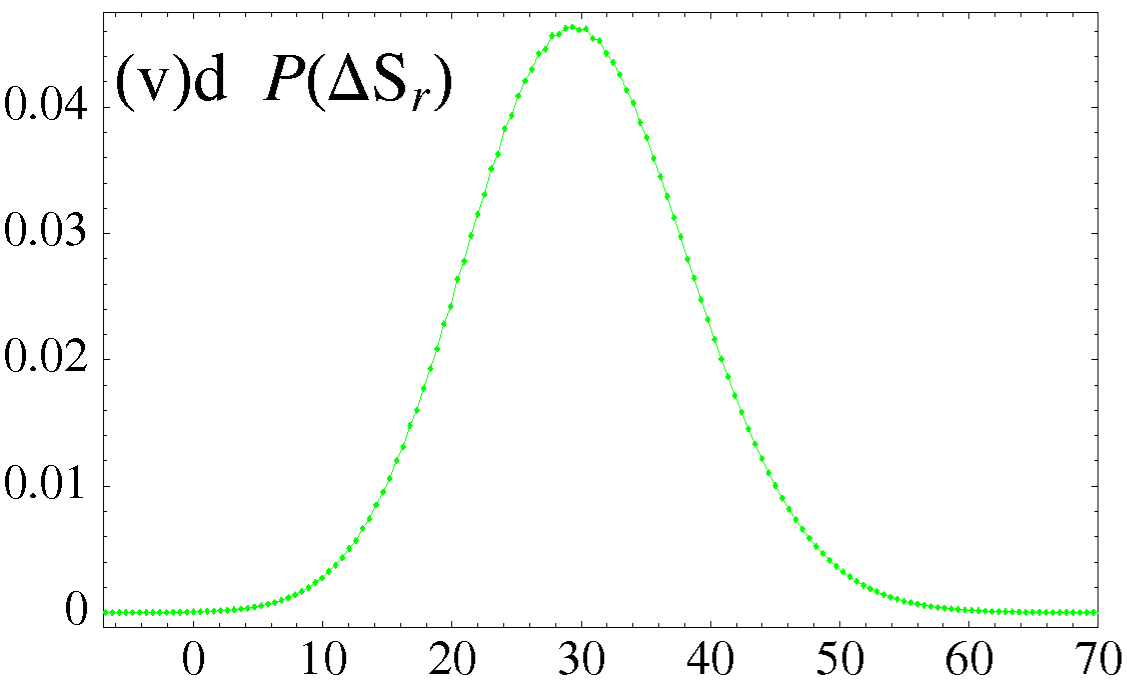
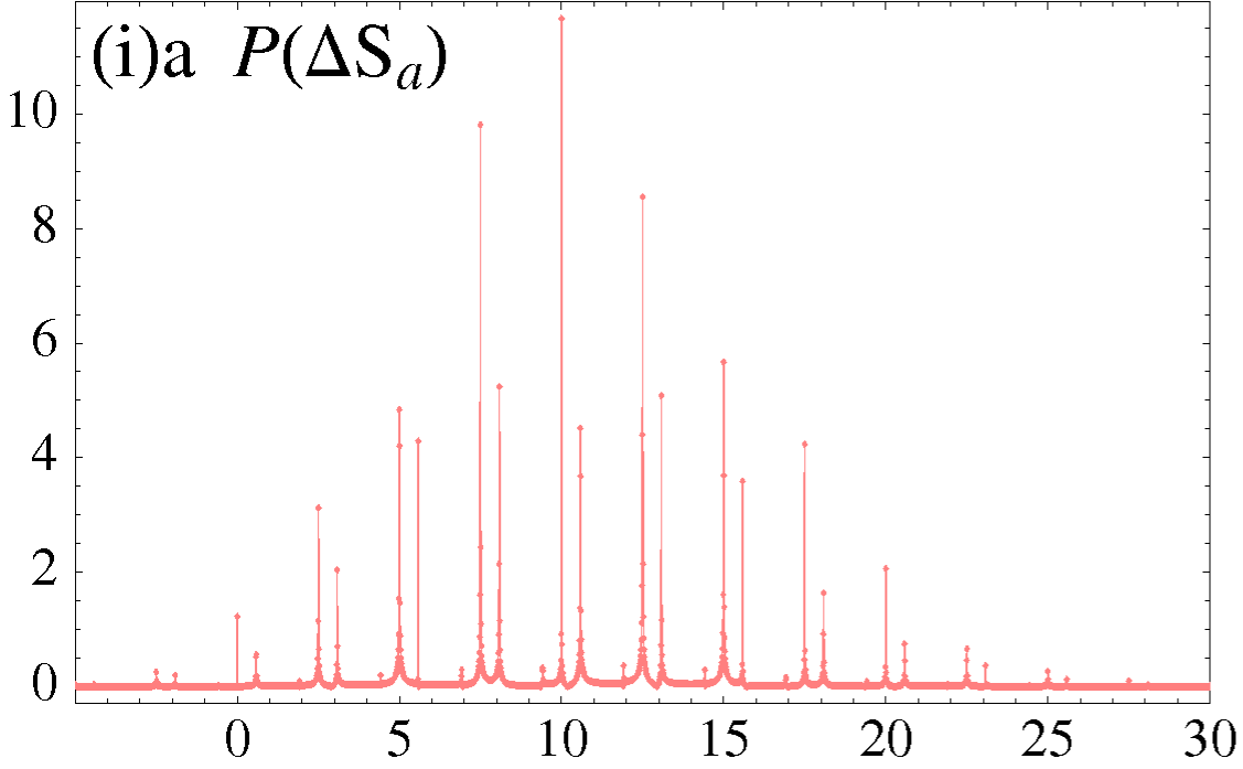
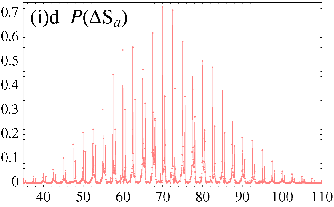
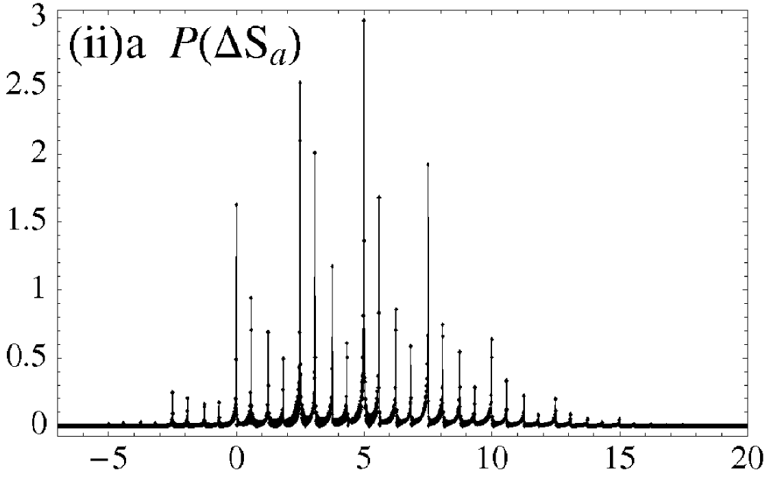
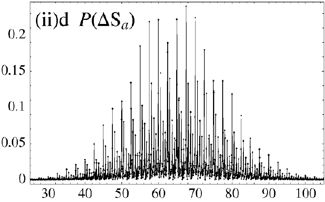
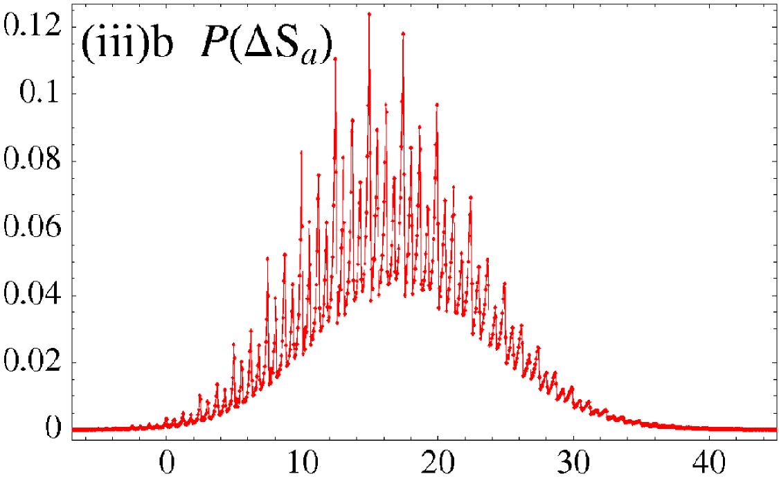
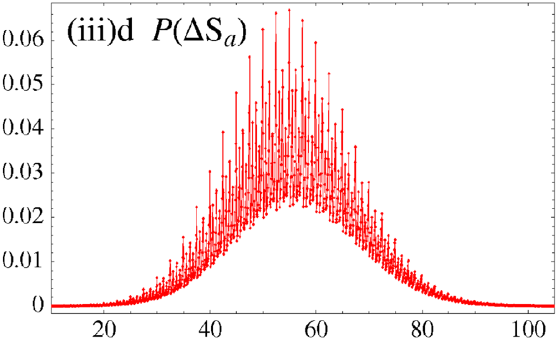
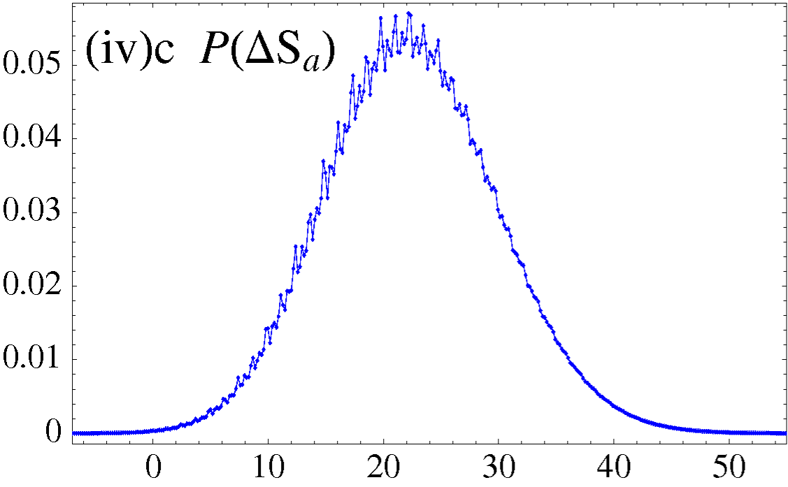
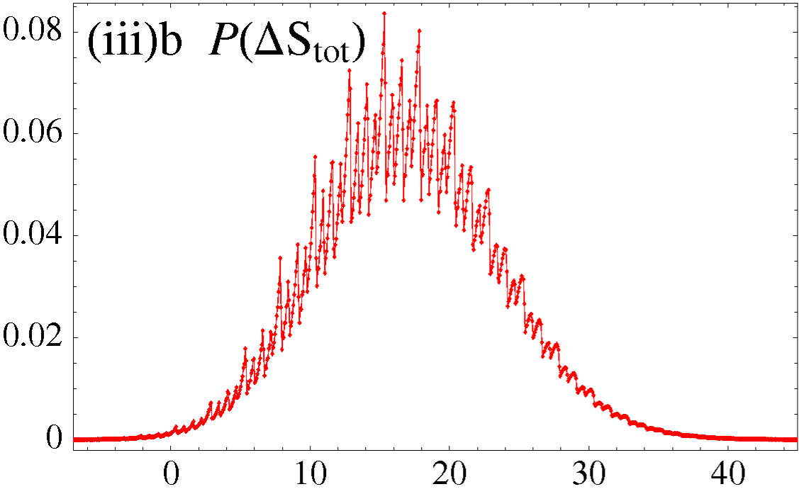
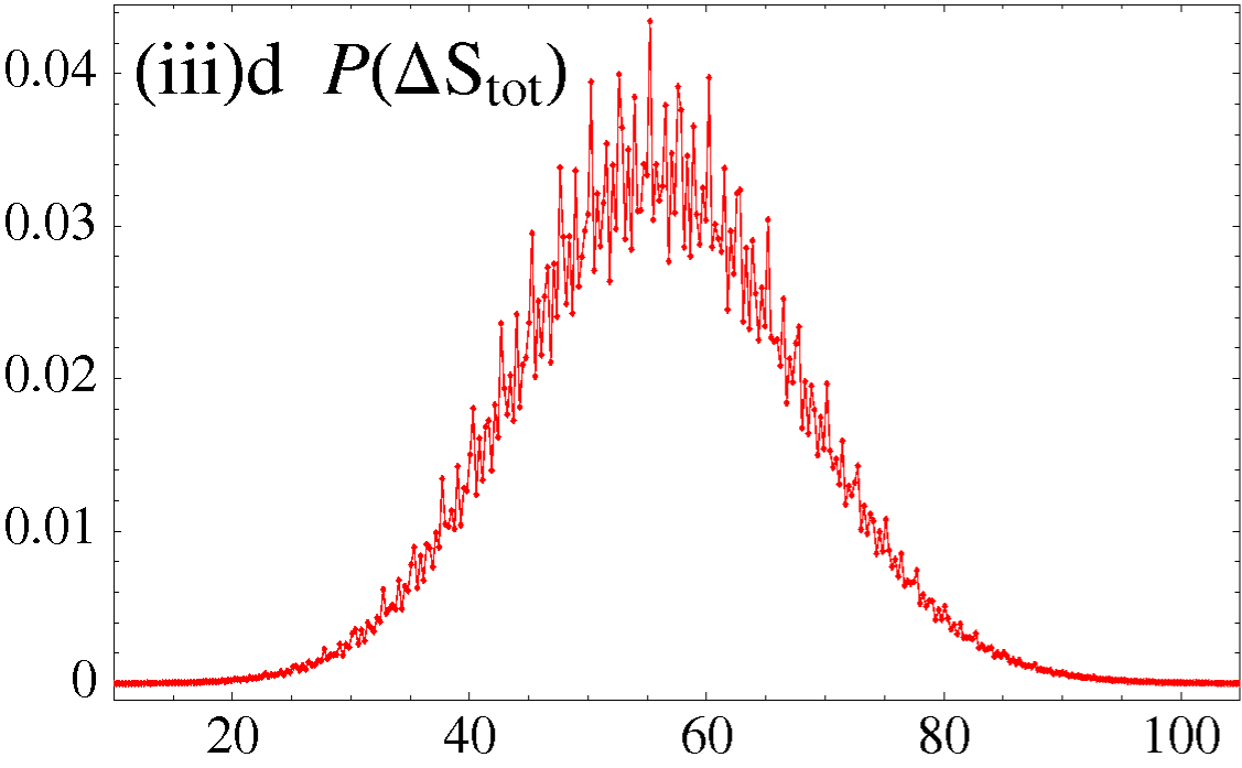
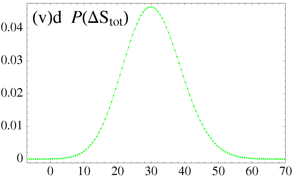
In Fig. 6, we display for different measurement times and protocols. Plots with same driving but different measurement times [(i)a and (ii)d or (ii)a and (ii)d or (iii)b and (iii)d] show the evolution of in the final steady state. The plots (ii)-(v) satisfy the FT (67) which for our parameters imply . The FT is not satisfied for (i) because the driving starts at the same time as the measurement [see section V.2.1]. To understand the structure of , we time integrate (40) and use the fact that in our model the heat current is proportional to the matter current between the reservoir and the system where
| (104) |
We get
| (105) |
In the sudden switch limit (i), we get
| (106) |
where is the net number
of electron transferred from the reservoir to the system between and .
This explains why in (i) only take discrete value which are multiples of each other.
The distance between the peaks of observed in (i) is due to
the right lead only because our
parameters are such that ].
The new peaks which appear in (ii) with a spacing are due
to the fact that the driving starts some time after the measurement
so that also contributes.
As the driving speed slows down (iii)-(v), the discrete structure
broadens and can take continuous values.
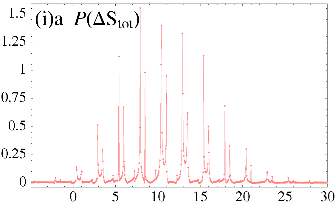
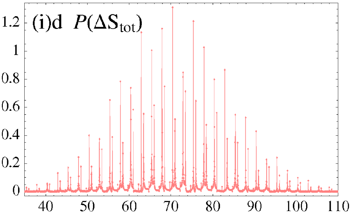
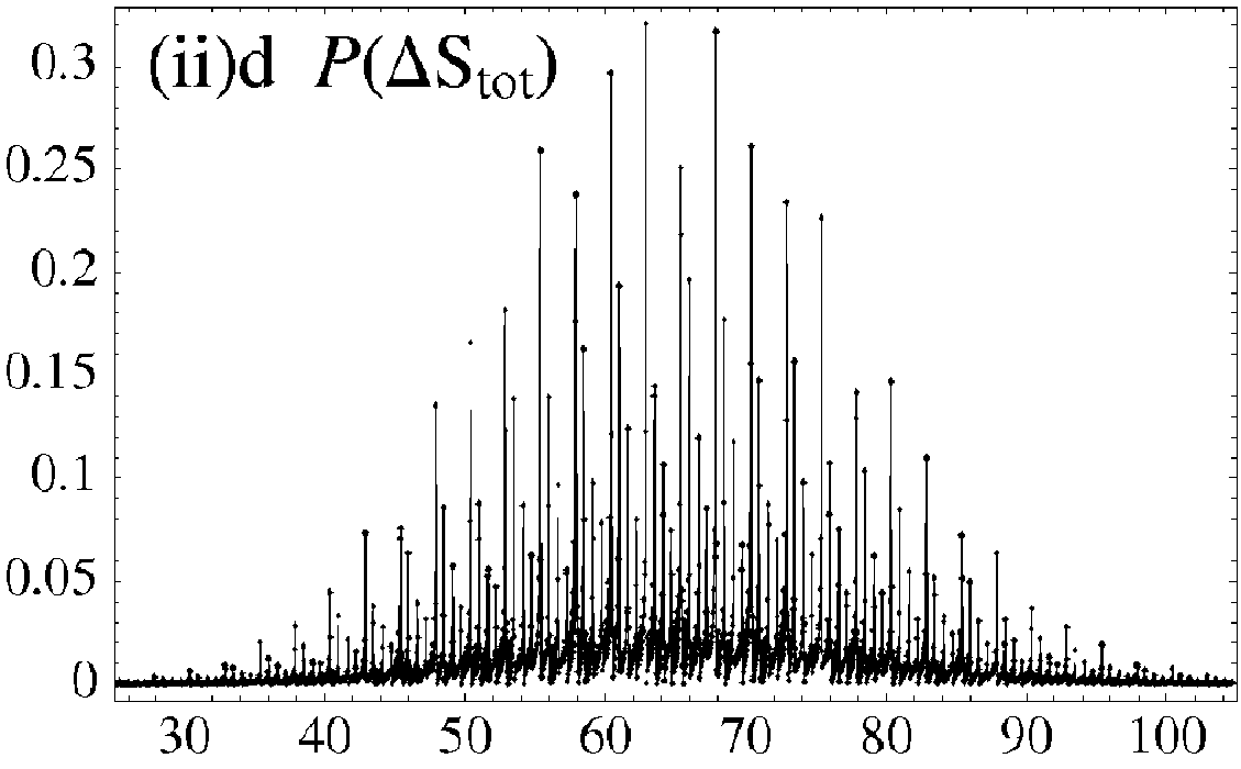
In Fig. 7, we display .
All curves satisfy the FT (61).
The verification (not shown) is best done on the GF () because the
numerical accuracy of the tail of the distribution is not sufficient.
The peak structure of can be understood from
and because .
This is particularly clear for the sudden switch (i) where
the possible values of the entropies are strongly restricted.
Indeed, in (i) each peak of is split in three smaller
peaks which have the same structure as .
As the speed of the driving decreases (ii)-(v), the peak structure disappears.
VII Conclusions
For a driven open system in contact with multiple reservoirs and described by a master equation, we have proposed a partitioning of the trajectory entropy production into two parts. One contributes when the system is not in its steady state and contains two contributions due to the external driving and the deviation from steady state in the initial and final probability distribution of the system. The second part comes from breaking of the detailed balance condition by the multiple reservoirs and becomes equal to the total entropy production when the system remains in its steady state all throughout the nonequilibrium process. Both parts as well as the total entropy production satisfy an general integral fluctuation theorem which imposes positivity on their ensemble average. This partitioning also provides a simple way to identify which part of the entropy production contributes during a specific type of nonequilibrium process [see Fig. 9]. Previously derived integral fluctuation theorems can be recovered from our three general fluctuation theorems and in addition we derived a new integral fluctuation theorem for the part of the entropy production due to exchange processes between the system and its reservoirs (reservoir entropy production). Our results strictly apply to systems described by a master equation (1). However, as has often be the case for previous fluctuation relations, one could expect similar results to hold for other types of dynamics. For electron transport trough a single level quantum dot between two reservoir with time dependent chemical potentials, we have simulated and analyzed in detail the probability distributions of the various trajectory entropies and showed how they can be measured in electron counting statistics experiments.
Acknowledgments
The support of the National Science Foundation (Grant No. CHE-0446555)
and NIRT (Grant No. EEC 0303389) is gratefully acknowledged.
M. E. is partially supported by the FNRS Belgium
(collaborateur scientifique).
Appendix A Fluctuation theorems in terms of forward backward trajectory probabilities
We show that the FT (59) and (60) have an interesting interpretation in
term of the ratio of the probability of a forward dynamics generating a given trajectory
and the probability of the time-reversed trajectory during some backward dynamics.
This is an alternative to the GF approach which connects the detailed
form to the integral form of the FTs.
The forward dynamics is described by the ME (1). We introduce the probability (in trajectory space) that the system follows a trajectory
The factors in
this expression represent the probability that the system undergoes
a given transition whereas the exponentials describe the probability
for the system to remain in a given state between two successive jumps.
Summation over all possible trajectories will be denoted
by . It consists of time-ordered integrations
over the time variables from
to (this gives the probability of having a path
with transitions) and then summing over all possible
from to .
Normalization in trajectory-space implies that
.
The backward dynamics is described on the time interval by the ME
| (108) |
where the new rate matrix satisfies . We require that the parametric time dependence (via the driving protocol ) of the rate matrix in Eq. (108) is time-reversed compared that of Eq. (1) and that the diagonal part of the rate matrix in Eq. (1) and (108) is the same
| (109) |
This still leaves room for different choices
of .
We will later specify two choice of
[(117) and (120)] that will result in two FTs.
We define the time-reversed trajectory of by
.
The probability
that the system described by (108) follows the
time-reversed trajectory is given by
where .
Normalization in the reverse path ensemble implies
.
We consider the ratio of the two probabilities (A) and (A),
| (111) |
Due to (109), the contributions from the exponentials (which represent the probabilities to remain on a given state) in (111) cancel, so that
| (112) |
We can partition (112) in the form
We assume for the moment that can be expressed
exclusively in terms of quantities of the dynamics (1)
i.e. a recipe has to be provided to express the tilde
quantities in (112) [ and
]
in terms of non-tilde quantities.
In analogy with (111), we define
| (114) |
for the tilde dynamics.
The previous recipe also implies that
can be exclusively expressed in terms of quantities of the tilde
dynamics (108).
Eq. (111) together with (114) implies that
.
The probability to observe a trajectory such that during the forward dynamics is related to the probability to observe a trajectory such that during the backward dynamics
By integrating over , we get
| (116) |
It follows from Jensen’s inequality
,
that .
We now make a first choice of in the backward dynamics (108)
| (117) |
In this case the backward dynamics is identical to the original one, except that the driving protocol is time reversed. If we also choose the initial conditions of the backward dynamics to be the final conditions of the forward dynamics , using (112) and (IV.1), we find
| (118) |
The FT (59) previously derived using GFs now follows from Eq. (116). Using (A), we also get the detailed form of the FT
| (119) |
We now make a second choices of in (108)
| (120) |
In the theory of MEs, (108) with (120) is called the time reversal ME of (1) Norris ; Stirzaker . We again choose the initial condition of the tilde dynamics to be the final conditions of the original dynamics . Using (A) with (120) and (IV.1), we get
| (121) |
The previously derived FT (60) follows now from (116). From Eq. (A) we find the detailed form of the FT
| (122) |
We can interpret the change in the total TEP during the to
time interval as the logarithm of the (forward) probability
that the driven system follows a given trajectory divided by the backward
probability that the system, initially in the final probability distribution
of the forward evolution, and driven in a time reversed way compared to the
forward evolution, follows the time-reversed trajectory.
The nonadiabatic TEP is interpreted as the logarithm of the (forward) probability
that the driven system follows a given trajectory divided by the backward probability
that the system, initially in the final probability distribution of the forward
evolution, and described by the time-reversed ME, follows the time-reversed trajectory.
It should be noted that the backward ME (108) with (120) is
different from the backward ME (108) with (117) only for systems
interacting with multiple reservoirs which break the DBC.
Only in this case (59) is different from (60).
References
- (1) D. J. Evans, E. G. D. Cohen, and G. P. Morriss, Phys. Rev. Lett. 71, 2401 (1993).
- (2) G. Gallavotti and E. G. D. Cohen, Phys. Rev. Lett. 74, 2694 (1995); J. Stat. Phys. 80, 931 (1995).
- (3) D. J. Evans and D. J. Searles, Phys. Rev. E 50, 1645 (1994); Phys. Rev. E 52, 5839 (1995); Phys. Rev. E 53, 5808 (1996).
- (4) C. Jarzynski, Phys. Rev. Lett. 78, 2690-2693 (1997); Phys. Rev. E 56, 5018-5035 (1997).
- (5) J. Kurchan, J. Phys. A 31, 3719 (1998).
- (6) J. L. Lebowitz and H. Spohn, J. Stat. Phys. 95, 333 (1999).
- (7) D. J. Searles and D. J. Evans, Phys. Rev. E 60, 159 (1999).
- (8) G. E. Crooks, Phys. Rev. E 60, 2721 (1999).
- (9) G. E. Crooks, Phys. Rev. E 61, 2361 (2000).
- (10) T. Hatano, Phys. Rev. E 60, R5017 (1999).
- (11) T. Hatano and S. I. Sasa, Phys. Rev. Lett. 86, 3463 (2001).
- (12) P. Gaspard, J. Chem. Phys. 120, 8898 (2004).
- (13) D. Andrieux and P. Gaspard, J. Chem. Phys. 121, 6167 (2004).
- (14) U. Seifert, Phys. Rev. Lett. 95, 040602 (2005).
- (15) T. Speck and U. Seifert, J. Phys. A: Math Gen. 38, L581 (2005).
- (16) V. Y. Chernyak, M. Chertkov, and C. Jarzynski, J. Stat. Mech. (2006) P08001.
- (17) B. Cleuren, C. Van den Broeck and R. Kawai, Phys. Rev. E 74, 021117 (2006).
- (18) C. Bustamante, J. Liphardt and F. Ritort, Physics Today 58, 43 (2005).
- (19) D. Andrieux and P. Gaspard, J. Stat. Mech. (2006) P01011.
- (20) J. Liphardt, S. Dumont, S. B. Smith, I. Tinoco (Jr), and C. Bustamante, Science 296, 1832 (2002).
- (21) E. H. Trepagnier, C. Jarzynski, F. Ritort, G. E. Crooks, C. J. Bustamante, and J. Liphardt, PNAS 101, 15038 (2004).
- (22) D. Collin, F. Ritort, C. Jarzynski, S.B. Smith, I. Tinoco (Jr), and C. Bustamante, Nature 437, 231 (2005).
- (23) F. Douarche, S. Ciliberto, A. Petrosyan and I. Rabbiosi, Europhys. Lett. 70, 593 (2005).
- (24) G. M. Wang, J. C. Reid, D. M. Carberry, D. R. M. Williams, E. M. Sevick, and D. J. Evans, Phys. Rev. E 71, 046142 (2005).
- (25) S. Schuler, T. Speck, C. Tietz, J. Wrachtrup, and U. Seifert, Phys. Rev. Lett. 94, 180602 (2005).
- (26) C. Tietz, S. Schuler, T. Speck, U. Seifert, and J. Wrachtrup, Phys. Rev. Lett. 97, 050602 (2006).
- (27) T. Fujisawa, T. Hayashi, R. Tomita, and Y. Hirayama, Science 312, 1634 (2006).
- (28) We assume an irreductible rate matrix Stirzaker ; Norris ; Kampen .
- (29) D. Stirzaker, Stochastic Processes and Models (Oxford University Press, 2005).
- (30) J. R. Norris, Markov Chains (Cambridge University Press, 1997).
- (31) N. G. van Kampen, Stochastic Processes in Physics and Chemistry, 2nd ed. (North-Holland, Amsterdam, 1997).
- (32) D. Kondepudi and I. Prigogine Modern thermodynamics (Wiley, Chichester, 1998).
- (33) S. R. de Groot and P. Mazur, Non-equilibrium thermodynamics (Dover, New York, 1984).
- (34) J. Schnakenberg, Rev. Mod. Phys. 48, 571 (1976).
- (35) Y. Oono and M. Paniconi, Prog. Theor. Phys. Suppl. 130, 29 (1998).
- (36) S. I. Sasa, H. Tasaki, cond-mat/0411052.
- (37) D. Andrieux and P. Gaspard, J. Stat. Phys. 127, 107 (2007).
- (38) L. S. Levitov and M. Reznikov, Phys. Rev. B 70, 115305 (2004).
- (39) A. L. Shelankov and J. Rammer, Europhys. Lett. 63, 485 (2003).
- (40) D. A. Bagrets and Yu. V. Nazarov, Phys. Rev. B 67, 085316 (2003).
- (41) Y. Utsumi, D. S. Golubev, and G. Schön, Phys. Rev. Lett. 96, 086803 (2006).
- (42) M. Esposito, U. Harbola and S. Mukamel , Phys. Rev. B. 75, 155316 (2007).
- (43) W. Lu, Z. Ji, L. Pfeiffer, K. W. West, and A. J. Rimberg, Nature 423 422 (2003).
- (44) T. Fujisawa, T. Hayashi, Y. Hirayama, H. D. Cheong, Appl. Phys. Lett. 84 2343 (2004).
- (45) J. Bylander, T. Duty, and P. Delsing, Nature 434, 361 (2005).
- (46) S. Gustavsson, R. Leturcq, B. Simovic, R. Schleser, T. Ihn, P. Studerus, K. Ensslin, D. C. Driscoll, and A. C. Gossard, Phys. Rev. Lett. 96, 076605 (2006).
- (47) C. W. J. Beenakker, Phys. Rev. B. 44, 1646 (1991).
- (48) E. Bonet, M. M. Deshmukh, and D. C. Ralph, Phys. Rev. B 65, 045317 (2002).
- (49) F. Elste and C. Timm, Phys. Rev. B 71, 155403 (2005).
- (50) S. Datta, Quantum transport: from quantum dot to transistor (Cambridge, New York, 2005).
- (51) B. Muralidharan, A. W. Ghosh, and S. Datta, Phys. Rev. B 73, 155410 (2006).
- (52) U. Harbola, M. Esposito and S. Mukamel, Phys. Rev. B. 74, 235309 (2006).

|
|

|

|
|

|
|
|

|
|
|
|
|
|

|
|
|
|
|
|
|
|
|
|
|
|
|
|
|
|
|
|
|
|

|
|
|
|

|
|