DCPT-07/35 A critical dimension for the stability of perfect fluid spheres of radiation

Abstract

An analysis of radiating perfect fluid models with asymptotically AdS boundary conditions is presented. Such scenarios consist of a spherical gas of radiation (a “star”) localised near the centre of the spacetime due to the confining nature of the AdS potential. We consider the variation of the total mass of the star as a function of the central density, and observe that for large enough dimensionality, the mass increases monotonically with the density. However in the lower dimensional cases, oscillations appear, indicating that the perfect fluid model of the star is becoming unrealistic. We find the critical dimension separating these two regimes to be eleven.

1 Introduction

There are numerous effects in physics which are dependent on the dimension of the spacetime in which they live, and concepts which have mathematically simple models when restricted to one or two dimensions may become intractably complex as the dimensionality increases. Furthermore, in some situations there is a sharp contrast in the behaviour of the system when the number of dimensions passes above or below a certain “critical dimension”. In the field of general relativity there are already some instances of such dimension dependent phenomena; for example, the Gregory-Laflamme instability [1, 2] of black strings, and the work of Belinsky, Khalatnikov and Lifshitz (BKL) [3] and its extensions [4, 5, 6], where the dynamics of a spacetime in the vicinity of a cosmological singularity were studied. In the latter case they found that the general behaviour of the relevant Einstein solutions changed from “chaotic” in the low dimensional cases to non-chaotic in higher dimensions. It is this extra complexity and appearance of a critical dimension which is discovered in the work presented here.

The issue of dimensionality has become of even greater importance over the past few decades, with the theories of hidden dimensions first postulated by Kaluza [7] resurfacing in the quest for unification and a Theory of Everything. Originally it was hoped one extra dimension would be sufficient; with the advent of string theory and its subsequent developments this was then expanded to twenty six in the late 1960’s as a consistency requirement for bosonic strings, before being reduced back down to ten with the introduction of supersymmetry in the 1980’s. The idea of holography also has its roots in dimensionality, and its most famous form, that of Maldacena [8], states a relation between string theory on a five-dimensional anti-de Sitter space, and a four-dimensional conformal field theory. Much work (see [9] for a review) has followed investigating spacetimes and conformal field theories of varying dimension and complexity.

Here we present an analysis into the stability of radiating perfect fluid spheres in an asymptotically anti-de Sitter spacetime. Due to the confining nature of the AdS potential, the spheres of radiation are self-gravitating, and thus we shall refer to them as “stars” in much of the following, although this is mainly used as a conveniently brief label, as it is only a toy-model approximation to a star at best.

We begin by giving the equations for a such a model in $d$-dimensions, before analysing the behaviour of the star’s total mass. We consider the variation of the total mass as a function of the central density, and observe that for large enough dimensionality, the mass increases monotonically with the density. However in the lower dimensional cases, oscillations appear (this was originally noted in the $d=5$ case in [10]), indicating that the perfect fluid model of the star is becoming unrealistic. We numerically find the critical dimension separating these two regimes to be $11.0$ (to three significant figures), and give an explicit relation, (11), between the spacetime dimension $d$ and the “saturation density” $\rho_{c}$, see section 3.1. The existence of local maxima at critical central densities (saturation points) in the lower dimensional cases indicates the appearance of instabilities in the model of the star, and point to unrealistic effects developing for $\rho_{0}>\rho_{c}$. We also provide a numerical analysis of the behaviour at large central density, in particular the self-similar behaviour that appears in dimension $d<d_{c}$; several parameters of our numerical model are then also determined analytically from a dynamical systems analysis of the behaviour, where we consider the expansion about a fixed point of the zero-cosmological constant solution.

The outline of the paper is as follows: we begin with a brief recap on perfect fluid models in general dimension in section 2. In section 3 we introduce the total mass as a function of the central density, analyse the progression of the saturation point with increasing dimension, and present the best fit formula, (11), which gives a value for the critical dimension. We also present further numerical results for the behaviour of the total mass at large central densities. In section 4 we give a dynamical systems analysis, following the methods in [11] and [13], which yields analytical expressions for several of the numerical results of the previous section. Finally, we conclude with a discussion of the results in section 5.

2 Perfect fluid models

Consider a general static, spherically symmetric $d$-dimensional AdS spacetime with metric:

$$ds^{2}=-k(r)dt^{2}+h(r)dr^{2}+r^{2}d\Omega_{d-2}^{2}$$ (1)

By considering a perfect fluid of a gas of radiation, one can obtain implicit expressions for $k(r)$ and $h(r)$ for a simple model of a “star” geometry. For a perfect fluid we have that the stress tensor is of the form:

$$T_{ab}=\rho(r)u_{a}u_{b}+P(r)(g_{ab}+u_{a}u_{b})$$ (2)

where $u^{a}$ is the $d$-velocity of a co-moving gas, and upon which we impose the further constraint that the matter be purely radiating; this sets $\rho(r)=(d-1)P(r)$ as it requires that $T_{ab}$ be traceless. One obtains the required metric by solving Einstein’s equation: $G_{ab}+\Lambda g_{ab}=8\pi G_{d}T_{ab}$, with the above stress tensor and a negative cosmological constant, as follows. The relevant components of Einstein’s equations in general dimension $d$ are given by:

$$G_{rr}=\left(\frac{d-2}{2}\right)\frac{(d-3)(k(r)-k(r)h(r))+rk^{\prime}(r)}{r^{2}\,k(r)}=\left(\frac{\rho(r)}{d-1}+\frac{(d-1)(d-2)}{2\,R^{2}}\right)h(r)$$ (3)

$$G_{tt}=k(r)\left(\frac{d-2}{2}\right)\frac{(d-3)(h^{2}(r)-h(r))+rh^{\prime}(r)}{r^{2}\,h^{2}(r)}=\left(\rho(r)+\frac{(d-1)(d-2)}{2\,R^{2}}\right)k(r)$$ (4)

where we have used that $\Lambda=-(d-1)(d-2)/(2R^{2})$, $P(r)=\rho(r)/(d-1)$, and set $8\pi G_{d}\equiv 1$ for convenience. We can infer the form of $h(r)$ from (4), as the $k(r)$ dependence cancels, and we find that $h(r)$ is given by:

$$h(r)=\left(1+\frac{r^{2}}{R^{2}}-\frac{m(r)}{r^{d-3}}\right)^{-1}$$ (5)

where $m(r)$ is a mass function related to the density via:

$$m(r)=\frac{2}{d-2}\int_{0}^{r}\rho(\acute{r})\acute{r}^{d-2}\,\mathrm{d}\acute{r}$$ (6)

In order to specify a form for $k(r)$, we recall the energy-momentum conservation equation, $\nabla_{\mu}T^{\mu\nu}=0$, which for a general perfect fluid without the radiation condition gives:

$$P^{\prime}(r)+\frac{k^{\prime}(r)}{2\,k(r)}(P(r)+\rho(r))=0$$ (7)

which can be re-arranged to give

$$k(r)=\left(\frac{\rho_{\infty}}{\rho(r)}\right)^{2/d}$$ (8)

in the radiation case, where we have introduced $\rho_{\infty}$, which is the leading coefficient of $\rho(r)$ at large $r$, and is given by $\rho_{\infty}\approx\rho(r)r^{d}$ as $r\rightarrow\infty$. Substituting $h(r)$ from (5) into (3) and eliminating $k^{\prime}(r)/k(r)$ using (7) then gives an equation in terms of $m(r)$, $\rho(r)$ and $\rho^{\prime}(r)$,.

$$\frac{(d-3)}{r^{2}}\left(1-\frac{1}{1+\frac{r^{2}}{R^{2}}-\frac{m(r)}{r^{d-3}}}\right)-\frac{2\rho^{\prime}(r)}{r\,\rho(r)\,d}=\frac{2\rho(r)+(d-1)^{2}(d-2)/R^{2}}{(d-1)(d-2)\left(1+\frac{r^{2}}{R^{2}}-\frac{m(r)}{r^{d-3}}\right)}$$ (9)

which couples with our equation for $m^{\prime}(r)$:

$$m^{\prime}(r)=\frac{2}{d-2}\,\rho(r)\,r^{d-2}$$ (10)

to give a pair of ODEs. For specified dimension $d$, these allow the geometry of the spacetime to be numerically generated when they are combined with the relevant boundary conditions: $m(0)=0$ and $\rho(0)=\rho_{0}$. The condition $\rho(0)=\rho_{0}$ specifies the central density of the gas, and we have that for fixed $R$, $\rho_{0}$ is the single free parameter of the system (pure AdS is recovered when $\rho_{0}=0$).

3 Total mass as a function of central density

Whilst mathematically one can work with this perfect fluid setup in any number of dimensions (including non-integer ones), one would also like to consider the appropriateness of doing so, given that we wish to use the geometry as the setup for a toy model of a star. In other words, is there any significant change in behaviour as the dimensionality of the model is altered. A particular quantity of interest in analysing the stability of the model is the total mass $M$ of the star, and as we have just seen, the mass and density profiles of our gas of radiation are determined by a single parameter: the central density of the gas, $\rho_{0}$.

To avoid possible instabilities such as those considered in the asymptotically flat case (in four dimensions) in [14], one would expect the total mass to increase monotonically with $\rho_{0}$. One could also expect the total mass to be bounded from above by some maximum value, analogous to the $4d$ asymptotically flat case where for a fixed size $R_{star}$, the maximum possible mass such a star can have is given by $M_{max}=4R_{star}/9$, a result found by Buchdahl in 1959 [15].

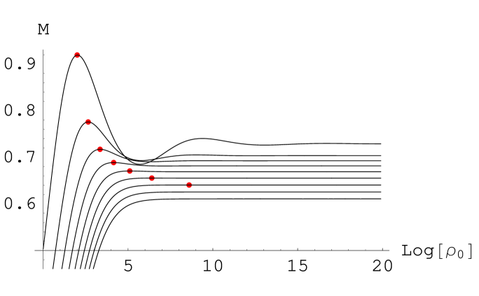
Fig. 1: Total mass vs density for the radiating perfect fluid model in various dimensions, from $d=4$ (top curve) through to $d=12$ (bottom curve). The saturation point for each dimension is indicated by the red dots; these correspond to the maximum value of the total mass in the relevant dimension, at the critical density $\rho_{c}$ (see section 3.1). For $d$ large, there is no local maximum and hence no finite saturation point; in these cases, the maximum total mass is given by the asymptotic value, $\eta_{d}$.

In our scenarios the total mass is indeed bounded from above, however, this maximum is not always the asymptotic value of the total mass at large density. Although we observe that as $\rho_{0}\rightarrow\infty$ we have $M(\rho_{0})\rightarrow\eta_{d}$, where $\eta_{d}$ is some finite constant dependent on the dimension $d$ (see section 3.2 below for more details), what we do not find in all cases is the total mass approaching this constant monotonically, see figure 1. When the dimensionality is low, there are sizable oscillations about the final value $\eta_{d}$ before the curve settles down (see figure 2), as was noted in the $d=5$ case in [10], and in other similar scenarios, e.g. [18], and the star’s maximum mass is given by some value greater than $\eta_{d}$. As the dimension is increased, however, these oscillations become less pronounced, and for $d$ sufficiently high they disappear altogether, see figure 3.

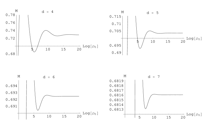
Fig. 2: The oscillations in the total mass $M$: as the central density $\rho_{0}$ is increased, $M$ does not simply increase monotonically towards its final value $\eta_{d}$. Instead, it reaches a larger maximum before undergoing damped oscillations towards $\eta_{d}$. Note that the amplitude of the oscillations becomes smaller as the dimensionality $d$ is increased.

Fig. 3: For larger $d$, there are no oscillations in the total mass: $M$ is now a monotonic function of the central density $\rho_{0}$, and its maximum is also its asymptotic value as $\rho_{0}\rightarrow\infty$, namely $\eta_{d}$.

Ideally one would like to analytically determine the dependence of the shape of the curve on both the dimension $d$ and the density $\rho_{0}$, however, due to the complexity of the equations, the exact behaviour must be computed numerically. One can nevertheless use this data to construct models of the various features of the star’s behaviour: for example, in section 3.2 below, we give an analysis of the total mass at large $\rho_{0}$ (where it approaches a constant, dependent on $d$) in different dimensions.

One particularly interesting feature is the appearance of the turning points in the total mass seen in figure 2, and specifically the locations of the local maxima in different dimensions. One can see from the figures that as the dimensionality is increased, the appearance of the first maximum moves to larger $\rho_{0}$; by analysing this progression one can obtain a remarkably simple relation which immediately gives a value for the critical dimension, above which the oscillations do not exist, and hence the total mass is a monotonic function of $\rho_{0}$.

3.1 A critical dimension

The saturation point, $\rho_{c}$, which we define as being the location of the first local maximum when increasing $\rho_{0}$, can be seen to progress to larger and larger $\rho_{0}$ as the dimension $d$ is increased, see figure 1. What we wish to determine is whether this saturation point appears for all dimension $d$ (for sufficiently large $\rho_{0}$), or whether there is a cut-off dimension, $d_{c}$, such that for larger $d$, there is no local maximum and hence no saturation point. Figure 4 shows how the saturation point varies with dimension; numerical analysis then finds (to 3 significant figures) that this behaviour is given by the following model:

$$\log{\rho_{c}}\approx 0.500\,d+\frac{5.75}{\sqrt{11.0-d}}-2.20$$ (11)

which gives a critical dimension $d_{c}=11.0$. What is perhaps rather surprising is the simplicity of (11): not only do we have a critical dimension appearing so clearly, the overall dependence on $d$ is remarkably simple, and the co-efficient of the linear term appears to be exactly one half.

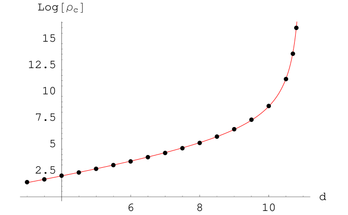
Fig. 4: The change in the saturation point $\rho_{c}$ with increasing dimension $d$. The points plotted are the calculated values for the saturation point for the star model in the corresponding dimension, the red best fit line is the curve given by (11). The divergent behaviour as $d$ approaches eleven indicates that for $d>11$ there is no saturation point, and hence no apparent instability in the perfect fluid model of the “star”.

As we shall see in section 4, the value of the critical dimension can also be determined by an analytical consideration of the radiating perfect fluid system with zero cosmological constant (i.e. in the limit $R\rightarrow\infty$). Although such a solution is singular at $r=0$, and has infinite mass, by confining the radiation to finite sized box one can obtain finite mass solutions. The features determined in this configuration can be related to equivalent behaviour in the asymptotically anti-de Sitter case (where the (finite) mass is confined by the AdS potential), and indeed exact values for certain parameters can also be computed. This same analysis is not restricted to the star geometries considered here, it can be used with any linear equation of state [11], or even more generally [13]. Before giving the analysis for our case of perfect fluid radiation, however, we firstly present further numerical results.

3.2 Total mass at large $\rho_{0}$

In addition to considering the variation of the saturation point for the star with dimension, one can also investigate the asymptotic behaviour of $M$ as $\rho_{0}$ becomes large. As mentioned in section 3, at large $\rho_{0}$, the value of the total mass tends to a constant, $\eta_{d}$, which is then only dependent on the dimension; the value of this constant decreases as $d$ increases. The values are plotted in figure 5 and despite the complicated appearance of the plot, a remarkably close fit for all dimensions is given by:

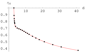
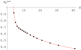
Fig. 5: The plot on the left shows $\eta_{d}$ for various dimensions, with the approximation given in (12) shown in red. The data points are all at integer values for the dimension, with the addition of points at $d=3.1,3.2,...,3.5$ to highlight the behaviour of the curve at low $d$. The righthand plot shows the behaviour of $M_{d}^{max}$; this is identical to that of $\eta_{d}$ for $d\geq 11$, however for $d<11$, the maximum is given by the value of the total mass at the saturation point, $\rho_{c}$. The best fit approximation (red curve) for each is simple in terms of its $d$ dependence, and provides a good fit over a large range of $d$.

$$\eta_{d}\approx 0.716+\exp\left[9.85-3.72\,d\right]-\exp\left[-0.603-\frac{20.3}{d}\right]$$ (12)

which is also shown in the figure. Checks show that the function continues to give accurate predictions for larger $d$, and although there is perhaps slightly more complicated behaviour for $d\sim 4$, we do not attempt to investigate this further here; despite the relative compactness of the expression, there is little intuitive origin for any of the constants involved. Nonetheless, it is impressive that the behaviour of the mass at large $\rho_{0}$ can be expressed in such simple powers of the dimension.

One can perform a similar analysis of the behaviour of the maximum value of the total mass as the dimension increases; the results are also shown in figure 5. For $d>11$, the maximum total mass corresponds to the asymptotic value, $\eta_{d}$, however, for lower dimension, the maximum is given by the mass at the saturation point. A good fit to the curve is given by:

$$M_{d}^{max}\approx 0.712+\exp\left[2.74-1.07\,d\right]-\exp\left[-0.592-\frac{20.5}{d}\right]$$ (13)

which differs (significantly) from (12) only in the second term; this was to be expected, as the curves differ only at low $d$. Whilst their is little apparent significance about the values of the numerical constants involved in the expression, we have again produced a fit with a relatively simple dependence on $d$ which gives accurate predictions for $M_{d}^{max}$ over a large range of dimensions.

Although the form of the fit used in equations (12) and (13) was chosen primarily because it gave such a close fit to the data, it would be interesting to study possible reasons for expecting the observed dependence on dimension, although we do not pursue this further here. What we do now examine in more detail, is the oscillatory behaviour, which can be considered both numerically and analytically.

3.3 Self-similarity analysis for $d<11$

Another interesting feature of the plots of the total mass seen in figures 1 and 2 is the self-similarity exhibited by the oscillatory behaviour as $\rho_{0}\rightarrow\infty$. A numerical analysis of the periodicity and damping of the oscillations seen for $3<d<11$ leads us to propose the following model for the total mass:

$$M_{d}(\rho_{0})\approx\eta_{d}+\alpha_{d}\exp\left[-\beta_{d}\,\log(\rho_{0})\right]\cos\left[\mu_{d}-\nu_{d}\log(\rho_{0})\right]$$ (14)

which gives a good approximation for the behaviour in the region $\rho_{0}>\rho_{c}$. In (14), $\eta_{d}$ is the asymptotic value of the mass discussed above, and the four parameters $\alpha_{d}$, $\beta_{d}$, $\mu_{d}$ and $\nu_{d}$ are constants dependent only on the dimension $d$. Approximate values for these constants for $d=3.1,4,5,6$ and $7$ are given in Table 1.

$d$	$\alpha_{d}$	$\beta_{d}$	$\mu_{d}$	$\nu_{d}$
3.1	0.305	0.184	8.33	0.66
4	0.383	0.371	8.44	0.86
5	0.400	0.601	9.35	0.98
6	0.415	0.825	10.3	1.03
7	0.431	1.03	11.4	1.07

Table 1: Numerical estimates for $\alpha_{d}$, $\beta_{d}$, $\mu_{d}$ and $\nu_{d}$ (to three significant figures) for the model of the total mass given in (14) .

Although the values given in table 1 are only approximate, we nonetheless see interesting dependencies on $d$ emerging. For example, $\beta_{d}$ appears to increase roughly linearly with dimension ($\beta_{d}\approx 0.22d-0.51$), as do $\alpha_{d}$ and $\mu_{d}$ for $d\geq 4$. We will see below in the dynamical systems analysis how this linear behaviour of $\beta_{d}$ on $d$ is only an approximation to the true behaviour, and the same analysis also provides exact values for the parameter $\nu_{d}$. This analytical analysis also confirms the form of the fit used in the numerical approximation derived above.

4 Dynamical systems analysis

By considering the behaviour of the system of coupled ODEs given in section 2 in the limit $R\rightarrow\infty$, we can obtain analytical results for some of the interesting features of the radiating perfect fluid star geometries described above. The analysis presented here follows that detailed in both [11] and [13], where it is given in more general settings; by focusing on the radiation case (where $\rho(r)=(d-1)P(r)$) we can give a good explanation of why the numerical behaviour seen above is so, without excessive over-complication.

The basic idea is to rewrite the equations for $\rho^{\prime}(r)$ and $m^{\prime}(r)$ in terms of dimensionless (compact) variables and perform an analysis of the fixed points. The corresponding eigenvalues and eigenvectors obtained by linearising about these fixed points give a complete description of the nearby behaviour (Hartman-Grobman theorem, [21]) on the new state space, which can then be translated back to the physical picture by inverting the transformations given below. Interestingly, for the perfect fluid stars, the dependence of the total mass (as well as other quantities, e.g. the entropy) on the central density, $\rho_{0}$, is governed by the behaviour around (and hence the eigenvalues of) a single fixed point. Specifically for our case we will see how this gives both an exact value for the critical dimension $d_{c}$, and a clear analytical explanation for the observed behaviour in the two regimes $d<d_{c}$ (oscillatory) and $d>d_{c}$ (monotonically increasing). We will also obtain expressions for the $\beta_{d}$ and $\nu_{d}$ parameters introduced earlier.

To proceed, we thus set $R=\infty$, and our equations (9) and (10) become:

$$\rho^{\prime}(r)=-\frac{\rho(r)\,d\left((d-3)(d-2)(d-1)m(r)+2r^{d-1}\rho(r)\right)}{2(d-2)(d-1)(r^{d-2}-r\,m(r))}$$ (15)

$$m^{\prime}(r)=\frac{2}{d-2}\,\rho(r)\,r^{d-2}$$ (16)

where $8\pi G_{d}$ has again been set equal to one. Note that we do not include the $d=3$ scenario here as it is a special case (due to the non-dynamical nature of gravity). We can now introduce the dimensionless variables:

$$u=\frac{2\,r^{d-1}\rho(r)}{(d-2)m(r)}$$ (17)

and

$$v=\frac{(d-1)\,m(r)}{2\,r^{d-3}}\left(1-\frac{m(r)}{r^{d-3}}\right)^{-1}$$ (18)

which allow equations (15) and (16) to be rewritten in the form:

$$\frac{du}{d\xi}=-u\left(1-d+u+\left(d-3+\frac{u}{d-1}\right)\left(\frac{v\,d}{d-1}\right)\right)$$ (19)

$$\frac{dv}{d\xi}=-v\left(d-3-u+\left(d-3-u\right)\left(\frac{2\,v}{d-1}\right)\right)$$ (20)

where we have also introduced the new independent variable $\xi=\ln(r)$. For the case of positive mass and density we’re considering here, both $u$ and $v$ are greater than zero (for non-zero $r$), and we make a final change of variables to the bounded $U$ and $V$ defined by:

$$U=\frac{u}{1+u}\,,\;\;\;\;\;\;V=\frac{v}{1+v}$$ (21)

which gives the system of equations:

$$\frac{dU}{d\lambda}=U(1-U)\left(d-1-dU-\left(2d-4+\frac{d-3}{d-1}\right)V+\left(2d-3+\frac{d(d-5)+3}{(d-1)^{2}}\right)UV\right)$$ (22)

$$\frac{dV}{d\lambda}=V(1-V)(3-d+(d-2)U)\left(1+\left(\frac{2}{d-1}-1\right)V\right)$$ (23)

where we have also introduced the independent variable $\lambda$, defined by:

$$\frac{d\lambda}{d\xi}=\frac{1}{(1-U)(1-V)}\;\;\;\;\;\Bigg{(}=(1+u)(1+v)\Bigg{)}$$ (24)

The fixed points of the system ((22) and (23)) are calculated in the usual fashion, by setting both $dU/d\lambda$ and $dV/d\lambda$ to zero and solving for $U$ and $V$; there are six in total, with eigenvalues then obtained from

$$\frac{d}{d\lambda}\left(\begin{array}[]{c}U\\ V\end{array}\right)=\left(\begin{array}[]{cc}\frac{\partial}{\partial U}\left(\frac{dU}{d\lambda}\right)&\frac{\partial}{\partial V}\left(\frac{dU}{d\lambda}\right)\\ \frac{\partial}{\partial U}\left(\frac{dV}{d\lambda}\right)&\frac{\partial}{\partial V}\left(\frac{dV}{d\lambda}\right)\end{array}\right)\Bigg{|}_{fp}\left(\begin{array}[]{c}U-U_{fp}\\ V-V_{fp}\end{array}\right)$$ (25)

where the matrix components are evaluated at the particular fixed point under consideration. A table of such eigenvalues is given in [11], where they are labelled $T_{1},\dots,T_{6}$; we do not list them all again here, however, as orbits in the interior of the state space $[0,1]^{2}$ originate from either $T_{2}$ or $T_{4}$ and converge to the fixed point $T_{3}$ (as is shown in [13]). This fixed point corresponds to the singular self-similar solution given by equation (2.14) of [11], and due to the scale invariance of the system one can consider the entire set of (positive mass) solutions as being represented by a single orbit from $T_{2}$ to $T_{3}$ (this is true for any linear equation of state, $P(r)=q\rho(r)$).

Although one cannot write an analytic expression for this orbit, one can obtain approximations by linearising about the fixed points. As discussed briefly earlier, as this zero-cosmological constant solution is singular, in order to produce finite mass solutions the radiation must be confined to an (unphysical) box; the two fixed points $T_{2}$ and $T_{3}$ thus represent solutions with $\rho_{0}=0$ and in the limit $\rho_{0}\rightarrow\infty$ respectively. The behaviour described by the linearisation about $T_{3}$ then reveals aspects of the large $\rho_{0}$ limit of the radiating stars (where the confining AdS potential results in the finite mass solutions without the need for any unphysical box), exactly what we analysed numerically in sections 3.2 and 3.3. This linearisation gives an explanation for the existence of a critical dimension and the differing behaviour seen in higher and lower dimensions, including quantitative expressions for $d_{c}$ and the $\beta_{d}$ and $\nu_{d}$ parameters of Table 1, as we shall now show.

Fixed point $T_{3}$ corresponds to the following values of $U$ and $V$:

$$U_{T_{3}}=\frac{d-3}{d-2}\,,\;\;\;\;\;\;V_{T_{3}}=\frac{2(d-1)^{2}}{2-4\,d+(d-1)d^{2}}$$ (26)

and has eigenvalues:

$$T_{3}^{\pm} =\frac{d(d-3)}{2-4\,d+(d-1)d^{2}}\left(1-d\pm\sqrt{\frac{(d-12)d^{2}+13\,d-18}{d-2}}\right)$$ (27)

$$\equiv k_{d}\left(1-d\pm\sqrt{\frac{(d-12)d^{2}+13\,d-18}{d-2}}\right)$$

where we denote the coefficient $k_{d}$ and observe that it is strictly positive for $d>3$. These eigenvalues govern the behaviour of the solution, and we immediately see that there are two distinct regimes; one where the expression inside the square root is negative, corresponding to the oscillatory behaviour seen in figure 2, and one where the expression is positive, resulting in the monotonic behaviour seen in figure 3. We thus obtain a value for the critical dimension given by the solution to:

$$(d_{c}-12)d_{c}^{2}+13\,d_{c}-18=0$$ (28)

which yields $d_{c}=10.964\dots$, complementary to the value of $d_{c}=11.0$ obtained numerically, although with the significance of being non-integer rather than exactly $11$; interestingly for any linear equation of state the value of $d_{c}$ is always in the range $10\leq d_{c}\leq 11$, see [11].

We can relate the asymptotic behaviour obtained from the state space picture to the physical quantities of mass and density via several auxiliary equations to those given above, specifically:

$$\frac{dr}{d\lambda}=(1-U)(1-V)r\,,\;\;\;\frac{dm}{d\lambda}=U(1-V)m$$ (29)

and

$$\frac{d\rho}{d\lambda}=-\frac{V\,d}{d-1}\left(1-U+\frac{U}{d-1}\right)\rho$$ (30)

Given expressions for $U$ and $V$ in terms of $\lambda$ (as obtained from an analysis of the behaviour around the fixed points, say), one can integrate the above to determine corresponding expressions for the mass, radius and density in terms of $\lambda$. There is, however, a simple way to see the dependence of the total mass $M_{d}$ on the central density $\rho_{0}$, which also reveals the origin of the $\beta_{d}$ and $\nu_{d}$ parameters of our numerical model in section 3.3.

Focusing then on the case where $d<d_{c}$, how does the imaginary term in (27) lead to the (self-similar) oscillatory behaviour manifest in the total mass at large $\rho_{0}$? This can be seen directly from the linearisation about $T_{3}$, where we observe similar oscillations in the expressions for $U(\lambda)$ and $V(\lambda)$ (see below); as mentioned above, it is the behaviour around $T_{3}$ that governs the behaviour of the physical quantities in the large $\rho_{0}$ limit. By considering the behaviour of $U(\lambda)$ and $V(\lambda)$ in terms of $\rho_{0}$, we can extract the coefficients which should then match those in (14) (as argued more fully in [13]). The solutions of (22) and (23) in the large $\lambda$ limit (i.e. about the fixed point $T_{3}$) can be expressed as:

$$Re(U(\lambda))=U_{T_{3}}+\exp\left(-(d-1)k_{d}\lambda\right)\cos\left(k_{d}\lambda\sqrt{\frac{18-(d-12)d^{2}-13\,d}{d-2}}\right)$$ (31)

$$Re(V(\lambda))=V_{T_{3}}+\exp\left(-(d-1)k_{d}\lambda\right)\cos\left(k_{d}\lambda\sqrt{\frac{18-(d-12)d^{2}-13\,d}{d-2}}\right)$$ (32)

where we have only kept the real angular term as we are only interested in the period of the oscillations ($\nu_{d}$) and the coefficient of the damping ($\beta_{d}$); the extra factors (namely $\alpha_{d}$ and $\mu_{d}$) cannot be extracted directly from this analysis.

For sufficiently high density stars (i.e. with large $\rho_{0}$), we have $\lambda\propto\frac{1}{2}\frac{d\lambda}{d\xi}\big{|}_{T_{3}}\log(\rho_{0})$, and we thus obtain:

$$\beta_{d}=\frac{(d-1)k_{d}}{2(1-U_{T_{3}})(1-V_{T_{3}})}=\frac{d}{4}+\frac{1}{2\,d}-\frac{3}{4}$$ (33)

and

$$\nu_{d} =\frac{k_{d}}{2(1-U_{T_{3}})(1-V_{T_{3}})}\sqrt{\frac{18-(d-12)d^{2}-13\,d}{d-2}}$$ (34)

$$=\frac{1}{4\,d}\sqrt{(d-2)(18-(d-12)d^{2}-13\,d)}$$

which give the values shown in Table 2, provided as a comparison to the numerical estimates obtained in section 3.3. We see that they match very closely, with any discrepancies most likely due to a combination of numerical imprecision in the original data for the mass at large $\rho_{0}$ and the use of oscillations at insufficiently large $\rho_{0}$ for the asymptotic dependence to be totally dominant.

$d$	$\beta_{d}$	$\nu_{d}$
3.1	$231/1240\approx 0.186$	$\sqrt{695519}/1240\approx 0.672$
4	$3/8=0.375$	$\sqrt{47}/8\approx 0.857$
5	$3/5=0.6$	$2\sqrt{6}/5\approx 0.980$
6	$5/6\approx 0.833$	$\sqrt{13/3}/2\approx 1.04$
7	$15/14\approx 1.07$	$2\sqrt{215}/5\approx 1.05$

Table 2: Exact values (alongside decimal equivalents) obtained from the dynamical systems analysis for $\beta_{d}$ and $\nu_{d}$ for the model of the total mass (14).

5 Discussion

What we have seen in the above analysis is firstly the appearance of a critical dimension ($d_{c}=11.0$) from the simple requirement of a stability condition on our perfect fluid model for a gas of radiation, and a numerical study of the behaviour in various dimensions. Whilst the appearance of oscillations in the variation of the total mass with the central density $\rho_{0}$ in the lower dimensional cases had been noted before, we saw here that such oscillations do not appear to persist in the higher dimensional cases (see figures 2 and 3). Not only do the oscillations die down as the dimensionality is increased, by analysing the progression of the saturation point, $\rho_{c}$, we find that they disappear completely for $d$ above a certain value. Although this value was calculated to be $11.0$ in the original numerical analysis, the dynamical systems approach which followed in section 4 not only gave a more precise, non-integer value ($d_{c}=10.964\dots$, as first derived in [11]), but also explained analytically why one sees a change from oscillatory to monotonic behaviour as one increases the dimension past this point. The section concluded by demonstrating how the $\beta_{d}$ and $\nu_{d}$ parameters of the numerical model could also be derived via this analytical approach.

What is remarkable is that from a seemingly basic condition (that of monotonicity in the variation of the total mass), one arrives at such a simple relation for the dependence of $\rho_{c}$ on $d$, namely equation (11). Such simplicity could not have been expected given the complex nature of the initial setup, which allows the spacetimes in question to be generated only numerically from the coupled ODEs. The extensions [4, 5, 6] to the BKL work on modelling a gravitational field close to a spacelike singularity also reveal a critical dimension of eleven. In their work they found that the general behaviour of the relevant Einstein solutions changed from “chaotic” in the low dimensional cases ($d<11$) to non-chaotic in higher dimensions ($d\geq 11$), in much the same manner as we observe the transition from oscillatory to monotonic total mass behaviour in the radiating star case considered here. It is interesting that their work also reveals a critical dimension of eleven, and a more detailed comparison of the two different scenarios (including an analysis to determine the exact (possibly non-integer) value of $d_{c}$ for their transition) may yield further insight.

It would be interesting to see if such a result appears in other investigations into scenarios similar to the radiating perfect fluid model considered here. For example, one could examine other physical equations of state to see if they exhibit the same behaviour, and indeed the work of [11] and [12] has pursued this idea further (see the note below). Finally, one could also look to explain the linear $d/2$ term which appears in (11), and whether there is any physical explanation for why the coefficient should take on the value of a half.

Note

Unknown to the author, this phenomenon has also been simultaneously investigated in two other works. In [11], Vladislav Vaganov analyses the behaviour of radiating perfect fluid models in $d$-dimensional AdS spacetimes; he notes (as we do here) that there is a significant change in the behaviour of the total mass for $d>11$ (where it becomes a monotonic rather than oscillatory function of the central density), and demonstrates this not only for the mass but also the temperature and entropy.

He also presents a dynamical systems analysis (based on that given in [13]) of the behaviour for a general linear equation of state, $P(r)=q\rho(r)$, which includes the radiation case. This analysis complements the numerical results presented here, providing an analytic derivation of the critical density, which is determined to be $d_{c}=10.964\dots$, consistent with our relation (11). The specific analysis for the radiation case is given in section 4, where we give not only the derivation of the critical density, but also demonstrate how the dynamical systems technique gives analytical expressions for other parameters introduced in our numerical investigation into the self-similar behaviour for $d<d_{c}$.

The second related paper, [12] by Pierre-Henri Chavanis, presents an in-depth study of the behaviour of general stars (“isothermal spheres”) with a linear equation of state in an asymptotically flat background. His results are again complementary, finding that there is monotonic behaviour for $d\geq 11$, in contrast to the oscillatory behaviour observed in lower dimensions. By asymptotic analysis he also finds the value for the critical dimension in the radiation case to be very close to eleven, and although there initially appeared to be a discrepancy between the two alternative calculations of the critical dimension in [11] and [12], the latter was subsequently corrected to agree with the value of $d_{c}=10.964\dots$ found in [11]. His paper also includes a comprehensive investigation into the stability of the different regimes, looking at a number of alternative stellar configurations and considering the behaviour of other thermodynamic parameters (entropy, temperature,$\dots$), in addition to the mass.

References

- [1] R. Gregory and R. Laflamme, “Black strings and p-branes are unstable”, Phys. Rev. Lett. 70, 2837 (1993) [arXiv:hep-th/9301052].
- [2] R. Gregory and R. Laflamme, “The instability of charged black strings and p-branes”, Nucl. Phys. B 428, 399 (1994) [arXiv:hep-th/9404071].
- [3] V. A. Belinsky, I. M. Khalatnikov and E. M. Lifshitz, “Oscillatory approach to a singular point in the relativistic cosmology”, Adv. Phys. 19, 525 (1970).
- [4] J. Demaret, M. Henneaux and P. Spindel, “Non-oscillatory behaviour in vacuum Kaluza-Klein cosmologies”, Phys. Lett. B 164, 27 (1985).
- [5] J. Demaret, J. L. Hanquin, M. Henneaux, P. Spindel and A. Taormina, “The Fate of the Mixmaster Behaviour in vacuum Inhomogeneous Kaluza-Klein Cosmological Models”, Phys. Lett. B 175, 129 (1986).
- [6] Y. Elskens and M. Henneaux, “Chaos in Kaluza-Klein models”, Class. Quant. Grav. 4, 161-167 (1987).
- [7] T. Kaluza, “On the problem of unity in physics”, Sitzungsber. Preuss. Akad. Wiss. Berlin (Math. Phys.) 966-972 (1921).
- [8] J. M. Maldacena, “The large N limit of superconformal field theories and supergravity”, Adv. Theor. Math. Phys. 2, 231 (1998) [Int. J. Theor. Phys. 38,1113 (1999)][hep-th/9711200].
- [9] O. Aharony, S. S. Gubser, J. M. Maldacena, H. Ooguri and Y. Oz, “Large N field theories, string theory and gravity”, Phys. Rept. 323, 183 (2000) [arXiv:hep-th/9905111].
- [10] V. E. Hubeny, H. Liu and M. Rangamani, “Bulk-cone singularities and signatures of horizon formation in AdS/CFT”, JHEP 0701, 009 (2007) [arXiv:hep-th/0610041].
- [11] V. Vaganov, “Self-gravitating radiation in AdS(d)”, arXiv:0707.0864
- [12] P. H. Chavanis, “Relativistic stars with a linear equation of state: analogy with classical isothermal spheres and black holes”, arXiv:0707.2292
- [13] J. M. Heinzle, N. Rohr and C. Uggla, “Spherically Symmetric Relativistic Stellar Structures”, Class. Quant. Grav. 20 (2003) 4567 [arXiv:gr-qc/0304012].
- [14] R. Sorkin, “A Criterion for the onset of instability at a turning point”, Astrophys. J. 249, 254-257 (1981).
- [15] H. A. Buchdahl, “General Relativistic Fluid Spheres”, Phys. Rev. 116 1027-1034 (1959).
- [16] J. M. Heinzle, “Bounds on 2m/r for static perfect fluids”, arXiv:0708.3352
- [17] M. Abramowicz, I. Bengtsson, V. Karas, K. Rosquist, “Poincare ball embeddings of the optical geometry”, Class. Quant. Grav. 19 3963-3976 (2002) [arXiv:gr-qc/0206027].
- [18] D. N. Page and K. C. Phillips, “Self-gravitating radiation in anti-de Sitter space”, GRG Vol. 17, No. 11 pp. 1029-1041 (1985).
- [19] C. Sire and P. H. Chavanis, “Thermodynamics and collapse of self-gravitating Brownian particles in D dimensions”, Phys. Rev. E 66 (2002) 046133 [arXiv:cond-mat/0204303].
- [20] J. Hammersley, “Numerical metric extraction in AdS/CFT”, arXiv:0705.0159
- [21] P. Hartman, “Ordinary Differential Equations”, Birkhäuser, Boston (1982). For an introduction to dynamical systems, see J. D. Crawford, “Introduction to bifurcation theory”, Rev. Mod. Phys. 63 4, 991-1038 (1991).