SN 1993J VLBI (IV): A Geometric Determination of the Distance to M81 with the Expanding Shock Front Method

Abstract

We compare the angular expansion velocities, determined with VLBI, with the linear expansion velocities measured from optical spectra for supernova 1993J in the galaxy M81, over the period from 7 d to $\sim$9 yr after shock breakout. The high degree of isotropy of the radio shell’s expansion, within 5.5%, with the projection of the radio shell being circular within even 1.4%, and the consistency of the radio shell thickness with predictions from hydrodynamic simulations and analytical computations argue strongly in favor of the radio-emitting shell being bound by the forward and reverse shocks. The absorption and emission of hydrogen at the highest velocity most likely also arise between the forward and reverse shocks, specifically in the shocked ejecta behind the contact surface which is close to the reverse shock, and possibly in Rayleigh-Taylor fingers that extend beyond it, farther out into the radio shell but not beyond the forward shock. The radio shell and the H$\alpha$ absorbing and emitting gas are on average similarly decelerated, but the latter slightly less so than the former several years after shock breakout. This may indicate developing Rayleigh-Taylor fingers, extending progressively further into the shocked circumstellar medium. We estimate the distance to SN 1993J using the Expanding Shock Front Method (ESM). We find the best distance estimate is obtained by fitting the angular velocity of a point halfway between the contact surface and outer shock front to the maximum observed hydrogen gas velocity. We obtain a direct, geometric, distance estimate for M81 of $D=3.96\pm 0.05\pm 0.29$ Mpc with statistical and systematic error contributions, respectively, corresponding to a total standard error of $\pm 0.29$ Mpc. The upper limit of 4.25 Mpc corresponds to the hydrogen gas with the highest observed velocity reaching no farther out than the contact surface a few days after shock breakout. The lower limit of 3.67 Mpc corresponds to this hydrogen gas reaching as far out as the forward shock for the whole period, which would mean that Rayleigh-Taylor fingers have grown to the forward shock already a few days after shock breakout. Our distance estimate is $9\pm 13$% larger than that of $3.63\pm 0.34$ Mpc from the HST Key Project, which is near our lower limit but within the errors.

1. INTRODUCTION

Supernova 1993J was discovered in a spiral arm of M81 south south-west of the galaxy’s center by Garcia (Ripero & Garcia, 1993) on 28 March 1993, shortly after shock breakout at $\sim$ 0 UT (Wheeler et al. 1993) on the same day ($t=0$ d). It subsequently became the optically brightest supernova in the northern hemisphere since SN 1954A and one of the brightest radio supernovae ever detected. It is also one of the closest extragalactic supernovae ever observed and is second only to SN 1987A as a subject of intense observational and theoretical supernova studies. This combination allows for sensitive spectroscopic and spectropolarimetric observations and for exceptionally detailed VLBI imaging, the latter giving us the highest relative resolution ever obtained for any radio supernova (Figure 1).

Combining the radial velocities of the ejecta gas obtained from the optical lines with the transverse angular velocities of the radio shell obtained from VLBI measurements yields a direct estimate of the distance to the supernova and its host galaxy. This method, called the Expanding Shock Front Method (ESM), was used to determine the distance to SN 1979C in M100 in the Virgo cluster (Bartel 1985; Bartel et al. 1985; Bartel & Bietenholz 2003, 2005). However the relatively large distance to Virgo has made it hard to resolve the supernova in sufficient detail, and an accurate distance estimate for Virgo is still pending.

In contrast, M81, the host galaxy of SN 1993J, is much closer. Its distance was recently determined via HST observations of Cepheids to be $3.63\pm 0.34$ Mpc (Freedman et al. 1994, see also Freedman et al. 2001, HST Key Project) and 3.93$\pm$0.26 Mpc (Huterer, Sasselov, & Schechter, 1995). Here we report on a detailed comparison between the angular velocities obtained from the VLBI measurements of the radio shell radius and the radial velocities obtained from the Doppler shifts of H$\alpha$, H$\beta$, He I, O[III], and Na I optical lines and determine the distance to SN 1993J and its host galaxy M81 with ESM.

This paper is the fourth in a series, presenting the results from our VLBI campaign on this supernova (see Bartel et al. 1994 for early results and Bartel et al. 2000 for an introduction of this series of results, see Marcaide et al. 1997 for parallel observations). In the first paper (Bietenholz, Bartel, & Rupen 2001; Paper I), we located the explosion center with respect to the nuclear radio source of M81, thus defining a stable reference point for our images. We also determined, using model-fitting, the motion of the geometric center of SN 1993J, and comment on the high degree of circular symmetry shown by SN 1993J. In the second paper (Bartel et al. 2002; Paper II), we determined the expansion speed of SN 1993J and measured its deceleration as a function of time. In the third paper, we presented a complete series of VLBI images of SN 1993J at 8.4 and 5.0 GHz, along with our latest image at 1.7 GHz (Bietenholz, Bartel, & Rupen, 2003; Paper III). In this fourth paper we use the main results of each of the previous papers, compare them with optical spectroscopic observations by others, include specific predictions from hydrodynamic simulations of this supernova for comparison with our observations, and determine directly the distance to M81.

In § 2, we summarize our VLBI observations and data reduction. In § 3 we describe the generic supernova shell model with its radio and optical emission regions and discuss the origin of the radio and optical emission and the relation of the forward and reverse shock to the measured boundaries of the radio emitting shell. In § 4 we elaborate on the expansion of the supernova as measured in the radio and optical wavelength range. Then we determine the distance to SN 1993J and its host galaxy in § 5, discuss our results in § 6 and finally give our conclusions in § 7.

2. OBSERVATIONS AND DATA REDUCTION

The observations were described in Papers I and II. To summarize, we observed SN 1993J at 34 epochs between 1993 and 2001 from $t=30$ to $\sim 3000$ d. At the earliest epoch, at $t=30$ d, we observed only at 22.2 GHz. At later epochs up to the $33^{\rm rd}$ epoch at $t=2996$ d, we observed mostly at 8.4 GHz and often also at 5.0 GHz. In addition, we also observed at some early epochs at 14.8 GHz and throughout the full eight years sporadically also at 2.3 and 1.7 GHz. We used a global array of between 9 and 18 telescopes with a total time of 9 to 18 hours for each session. We have continued observing SN 1993J at approximately one-year intervals and will report on these observations in future papers.

The data were recorded with either the MK III or the VLBA/MKIV VLBI systems, and correlated with the NRAO VLBA processor in Socorro, New Mexico, USA. We refer the interested reader to Paper II where details of the observing sessions are tabulated. The analysis was carried out using NRAO’s Astronomical Image Processing System (AIPS).

Most of our observations were phase-referenced to M81^∗, the radio source in the center of the galaxy M81. Being very compact (Bietenholz et al. 1996), M81^∗ is an excellent calibrator for phase-referenced mapping. Our images are among those with the lowest background noise level currently obtained with VLBI. Bietenholz, Bartel, & Rupen (2000) located a fixed point in the variable brightness distribution of M81^∗ that also has an inverted radio spectrum (Bietenholz, Bartel, & Rupen 2004a). We identified this point with the purported supermassive black hole in the center of the galaxy. Using this point as a reference point allowed us to locate the explosion center of SN 1993J on each of our supernova images with high precision.

In Figure 1 we show the galaxy M81 at optical wavelengths. Overlayed is an image of the galaxy at radio wavelengths, with SN 1993J clearly visible in a southern spiral arm. On the right side of the figure we show the VLBI image of the evolved radio shell which has the highest relative resolution obtained so far (Paper III).

In addition to imaging, we used model-fitting. We fit, by weighted least-squares, the two-dimensional projection of a three-dimensional spherical shell of uniform volume emissivity to the calibrated $u$-$v$ data consistently for all epochs. The ratio of the outer to inner angular radius was fixed at $\theta_{\rm o}$/$\theta_{\rm i}$= 1.25. From this fit, we estimated the shell’s center coordinates, $x,~{}y$, (see Paper I), and $\theta_{\rm o}$ (see Paper II). The shell’s center coordinates were found to be equal, within an rms of 64 $\mu$as, to those of the explosion center of SN 1993J. In the image in Figure 1 this center is at the origin. In addition, for relatively late epochs, we also determined the shell thickness by freeing the ratio of the radii and estimating $\theta_{\rm o}$ and $\theta_{\rm i}$ independently.

3. THE GENERIC SUPERNOVA SHELL MODEL AND ITS RELEVANCE FOR ESM

To clarify the astrophysical interpretation of the radio shell and its relation to the optical absorption and emission by the ejecta, we copied the left part of the VLBI image from Figure 1 and juxtaposed it to a sketch of a generic supernova shell model in Figure 2. The model describes a supernova expanding into the circumstellar medium (CSM) left over from the progenitor star. The supernova ejecta are spherically, freely expanding away from the explosion center for a large range of radii, $r$, from that center. Their temperature is $\sim 10^{4}$ K. The ejecta in the outermost regions hit the CSM, and a contact surface forms between the two media at a radius, $r_{\rm cs}$. From this surface, a forward shock, located at a radius, $r_{\rm fs}$, travels into the CSM and heats it up to $\sim 3\times 10^{8}$ K. Outside the forward shock, the CSM is unshocked and has a relatively high temperature of 10⁵ to 10⁶ K (Lundqvist & Fransson 1988; Fransson & Björnsson 1998; Mioduszewski, Dwarkadas, & Ball 2001). Also, a reverse shock travels from the contact surface back into the ejecta to a radius, $r_{\rm rs}$, from the explosion center and heats up the shocked ejecta to a temperature of $\sim 10^{7}$ K. The contact surface itself is Rayleigh-Taylor unstable, and fingers of ejecta are expected to develop and extend into the shocked CSM. These fingers are also sketched in Figure 2.

This general scenario above was described mathematically by the mini-shell model of self-similar expansion (Chevalier 1982a, b; see also Fransson, Lundqvist, & Chevalier 1996). This model assumes power-law density profiles for both the ejecta and the CSM, with $\rho_{\rm ej}\propto r^{-n}$ ($n>$5), and $\rho_{\rm CSM}\propto r^{-s}$. With this assumption, the expansion is self-similar, and the shock radius is given by $r_{\rm fs}\propto t^{m}$, where $m$ is the deceleration parameter, which is constant and is given by $m=(n-3)/(n-s)$. A hydrodynamic model for SN 1993J by Mioduszewski et al. (2001), based on an ejecta model by Shigeyama et al. (1994) (see also Suzuki & Nomoto 1995), relaxed the assumption of a power-law density profile in the ejecta. This model described the expansion of SN 1993J in more detail, and accounted for the deviations from self-similar expansion which were found for this supernova (Paper II).

The Expanding Shock Front Method is based on the transverse velocity of the Rayleigh-Taylor unstable contact surface being equal to the largest radial velocity of the ejecta. Dividing the latter by the former gives a geometric determination of the distance to the supernova and its host galaxy. In the following we will describe how the contact surface velocity distorted by Rayleigh-Taylor instabilities is related to the expansion velocity of the outer surface of the radio shell and how it compares with the maximum velocities measured in optical lines of the ejecta.

3.1. The origin of the radio emission

3.1.1 The forward and reverse shocks

It is believed that the forward shock accelerates electrons to ultrarelativistic velocities. These relativistic electrons then interact with the magnetic field amplified near the Rayleigh-Taylor unstable contact surface (e.g., Chevalier, Blondin, & Emmering 1992; Jun & Norman 1996a, b). This interaction leads to radio synchrotron radiation. Radio emission is therefore expected to originate in the shell region of the shocked CSM and likely also the shocked ejecta, i.e., in a region bound by $r_{\rm rs}$ and $r_{\rm fs}$. No radio emission is expected from the freely expanding, unshocked ejecta. Radio emission could also originate from a central compact source associated with the stellar remnant of the explosion, namely a neutron star or a black hole. Although a compact source was indeed found inside the shell of SN 1986J (Bietenholz, Bartel, & Rupen 2004b), no emission from such a source has yet been detected for SN 1993J or any other modern supernova (e.g., Bartel & Bietenholz 2005).

How can our radio images of SN 1993J be interpreted in detail in the context of this astrophysical model? The radio image of SN 1993J in Figure 1 shows an exemplary shell of emission. In general, the outer angular radii, $\theta_{\rm o}$ of our geometric shell model could be determined with an accuracy of about 1 to 2% and, for our latest images, the mean ratio of the outer to inner shell radii, $\theta_{\rm o}$/$\theta_{\rm i}$, to within 1% (Paper II). In Figure 2 we plot the fit geometric shell model as overlayed concentric circles with radii of $\theta_{\rm o}$ and $\theta_{\rm i}$. The center of the model circles is at the explosion center within 64 $\mu$as which corresponds to only about 1% of $\theta_{\rm o}$ (Paper I). Our finding that the radio emission can be so well fit by a spherical shell centered at the explosion center strongly supports the expectation that the fit angular radii, $\theta_{\rm o}$ and $\theta_{\rm i}$, indeed correspond to the radii of the forward and reverse shocks, $r_{\rm fs}$ and $r_{\rm rs}$, respectively. Other supernovae may not show such exemplary shells of emission and would therefore not be as good examples to show the close relationship between the radio shell boundaries and the forward and reverse shocks although that relationship most likely also exists given the example of SN 1993J.

3.1.2 The thickness of the radio shell and its relation to the forward and reverse shocks

Both the self-similar mini-shell model and the hydrodynamic model make predictions as to the distance between the forward and the reverse shocks. During the first months, when $m=0.92$ (Paper II), the ratio between the forward and reverse shock radii is predicted to be $1.19$ for $s=2$ for the self-similar mini-shell model. For a larger deceleration the shell thickness is predicted to be larger. For instance, with the mean of $m$ for the whole observing time up to $t\sim 3000$ d of $m=0.83$ (Paper II), a ratio of $1.30$ is predicted by the self-similar mini-shell model for $s=2$ (Chevalier & Fransson 1994).

Similar and most likely more reliable values for the shell thickness are predicted by the hydrodynamic model. In fact, Dwarkadas & Chevalier (1998) found that the shell thickness is relatively independent of the form of the ejecta profile for a long time after shock breakout, further supporting its robustness. In Figure 3 we plot the ratio of the forward and reverse shock radii from a few days to several years after the explosion as derived from the hydrodynamic simulations. The ratio increases from 1.16 between $t=10$ d and 20 d to an average of $1.29$ between $t=1000$ d and $3000$ d. In addition we plot our measurements from VLBI observations, $\theta_{\rm o}$/$\theta_{\rm i}$, determined at epochs from $t=996$ d onward when the radio shell was large enough to allow useful determinations. The mean of $\theta_{\rm o}$/$\theta_{\rm i}$ for epochs up to $t=2996$ d after the explosion was $1.29\pm 0.01$, with a slight broadening of the shell (significant only at the $1\sigma$ level, see Paper II), in good agreement with the models. This good agreement is additional evidence that the radio shell is indeed bound by the forward and reverse shocks.

3.1.3 The brightness profile of the shell and its relation to the forward and reverse shock

Below the image of the half radio shell in Figure 2 we plot the profile of the fit geometric shell model in several aspects. The data points give the observed profile. The solid curve gives the fit to the data of a (projected) shell model with uniform emissivity between $\theta_{\rm i}$ and $\theta_{\rm o}$ and partial absorption inside $\theta_{\rm i}$ (Paper III). The rectangular lines give the profile in the (unprojected) cross section of the shell. Clearly, the emission and the region where the emission originates is very well fit by our geometric model. In Paper III we reported on the steepness of the outer edge of the profile and found that it is indeed consistent with being an ideally sharp edge as in our model. However softer boundaries are not excluded. Nevertheless, the measured brightness profile can be taken as further evidence that the radio shell is indeed bound by the forward and reverse shocks, and that the parameters $\theta_{\rm i}$ and $\theta_{\rm o}$ therefore most likely correspond closely to $r_{\rm rs}$ and $r_{\rm fs}$.

On the right side of Figure 2 we sketch the minishell model and complete the concentric circles by indeed assuming here and hereafter that $\theta_{\rm i}$ and $\theta_{\rm o}$ correspond exactly to $r_{\rm rs}$ and $r_{\rm fs}$.

3.2. The origin of the optical emission

While optical continuum emission of the supernova is expected to mostly originate, at least at early times, from the photosphere in the central region of the expanding gas, optical emission and absorption in broad spectral lines is expected to arise in the gas of the hot ejecta, above the cooler and mostly neutral ejecta (Figure 2. In particular, emission was discussed as coming from a) the freely expanding ejecta and being caused by the heating and ionizing radiation from the interaction region, as well as from b) the shocked ejecta and being linked to radiative cooling (Chevalier & Fransson, 1994, and references therein). The ionizing luminosity and the density of the gas both change with time and give rise to evolving spectra. Blending of lines is common, and since the relative luminosities change with time, the degree of blending can change as well. The highest expansion velocity in absorption and emission lines is expected from the shocked gas of the envelope of the progenitor star, in a region that extends outwards to the Rayleigh-Taylor unstable contact surface at radius $r_{\rm cs}$. The highest observed optical expansion velocity could be smaller. No optical line emission is expected from the region of shocked CSM, i.e., beyond the contact surface between $r_{\rm cs}$ and $r_{\rm fs}$, since the temperature there is expected to be $\sim 3\times 10^{9}$ K.

3.3. The contact surface

3.3.1 The location of the contact surface within the radio shell

The location of the contact surface in relation to the forward and reverse shocks, i.e., to the outer and inner radio shell surfaces, is estimated by combining VLBI measurements of the radio shell thickness with circumstellar interaction models. Both the self-similar mini-shell model and the hydrodynamic model make predictions as to the distance between the contact surface and the reverse shock. During the first months, when $m=0.92$, the ratio between the contact surface and reverse shock radii is predicted to be $1.0065$ for $s=2$ by the self-similar mini-shell model. For a larger deceleration, e.g., for a mean of $m=0.83,s=2$ as taken before for a comparison (§ 3.1.2), the ratio is $1.03$ (Chevalier & Fransson 1994). The hydrodynamic model predicts a ratio similarly close to unity during the first month which then increases to a mean value of about 1.04 between $t\sim 1000$ and $\sim 3000$ d.

We parametrized $\theta_{\rm i}$ for the range of our radio and the optical observations by $\theta_{\rm i}$= $A_{\rm rf}t^{m_{\rm rf}}$ $\theta_{\rm o}$, where $t$ is the time since explosion in days. With $A_{\rm rf}=0.914$ and $m_{\rm rf}=-0.0217$, this parametrization gives a time-varying shell thickness consistent with the hydrodynamic simulations with, e.g., $\theta_{\rm o}$/$\theta_{\rm i}$ = 1.16 at $t=15$ d and 1.29 at $t=3000$ d (see Figure 3). These values are also fairly consistent with the predictions from the self-similar mini-shell model. (We also parametrized the angular radius of the contact surface by $\theta_{\rm c}$= $A_{\rm cf}t^{m_{\rm cf}}$ $\theta_{\rm o}$ with $A_{\rm cf}=0.904$ and $m_{\rm cf}=-0.0150$ to give $\theta_{\rm c}$ being 0.65% and 4% larger than $\theta_{\rm i}$ at $t=15$ d and 2500 d, respectively, as predicted by the above models.

3.3.2 Distortion of the contact surface by Rayleigh-Taylor instabilities

However, since the contact surface is decelerating, it is expected to be Rayleigh-Taylor unstable (Gull 1973; Chevalier 1982b), and that with time fingers of shocked ejecta will extend into the shocked CSM. A linear analysis of self-similar solutions as well as two-dimensional numeric hydrodynamic computations have shown that Rayleigh-Taylor instabilities are limited by Kelvin-Helmholtz instabilities but can still grow in length to generally 30 to 50% of the width of the shocked shell (Chevalier et al. 1992; Dwarkadas 2000). Under particular circumstances, when vortices are amplified by the magnetic field, it was shown that the fingers may even reach slightly beyond the outer shock, which is otherwise assumed to be spherically symmetrical (Jun & Norman 1996a, b). Also, for fast shocks with efficient particle acceleration and resulting high compression ratios, the width of the shocked shell was found to shrink considerably so that fingers, without growing much larger, could also reach and even slightly exceed the average forward shock radius (Blondin & Ellison 2001).

3.3.3 The fastest parts of the ejecta

The ejecta with the highest velocity are therefore located in the evolving Rayleigh-Taylor fingers stretching out beyond $r_{\rm cs}$ toward the forward shock at $r_{\rm fs}$. The fingers are expected to be less developed a few days after shock breakout and more developed a few years thereafter. Thus, the highest possible velocities in optical lines are those from the front of the Rayleigh-Taylor fingers which, depending on evolution time, stretch out to between $r_{\rm cs}$ and $r_{\rm fs}$ with an assumed mean, $r_{\rm x}=\text@frac{1}{2}(r_{\rm fs}+r_{\rm cs})$, which corresponds to an angular extent of $\theta_{\rm x}$.

4. THE EXPANSION

4.1. The angular expansion velocities of different surfaces of and within the radio shell

We used the values of $\theta_{\rm o}$ obtained from our VLBI observations to compute the angular expansion velocity of the outer surface of the radio shell, i.e., of the forward shock, $\dot{\theta}_{\rm o}$, as a function of time. The values of $\theta_{\rm o}$ were already listed and plotted in Paper II, but for the convenience of the reader we repeat the plot of $\theta_{\rm o}$ as a function of time here in Figure 4. It can be clearly seen that the outer surface of the radio shell is only slightly decelerated up to $t\sim 300$ d and from then on more strongly decelerated. Further, as can be seen from the inset of Figure 4, the deceleration changes significantly even after $t\sim 2000$ d (see also Paper II).

Because the expansion has an approximate power-law form, a linear fit to the values of $\theta_{\rm o}$ over a time interval would produce a biased estimate of $\dot{\theta}_{\rm o}$ at the midpoint of the interval. To avoid this bias, we computed $\mbox{$\dot{\theta}_{\rm o}$}(t)$ by first fitting a running solution of the form $\mbox{$\theta_{\rm o}$}=At^{m}$ to the data points near $t$, where we fit both the deceleration parameter, $m$, and the angular size scale, $A$. Our running solution is equivalent to a running mean, but instead of computing the weighted average in a shifting interval we computed the weighted linear fit in a shifting interval in a log-log diagram (see Paper II for more details). As our value of $\mbox{$\dot{\theta}_{\rm o}$}(t)$, we take the derivative of this fitted function, $Amt^{m-1}$, evaluated at the midpoint of the fitting interval on a logarithmic scale.

We extrapolated the angular velocity values slightly beyond the mean times of the first and last running solutions to cover the time range from $t\sim 5$ to $\sim 3000$ d. We plot the values of $\dot{\theta}_{\rm o}$ and connect them by lines in Figure 5. We also estimate standard errors from the power-law fits. These errors are between 1 and 5% of $\dot{\theta}_{\rm o}$. We plot them also in Figure 5. We further compute the angular velocity of the inner surface of the radio shell, i.e. of the reverse shock, $\dot{\theta}_{\rm i}$, the velocity of the contact surface, $\dot{\theta}_{\rm c}$, and the mean between the velocity of the contact surface and that of the forward shock, $\dot{\theta}_{\rm x}$, and also plot them in Figure 5. The ratios of the parametrized velocities, $\dot{\theta}_{\rm o}$/$\dot{\theta}_{\rm i}$ and $\dot{\theta}_{\rm o}$/$\dot{\theta}_{\rm c}$, are comparable to those from the hydrodynamic simulations after the latter are smoothed over appropriate time intervals.

4.2. The radial expansion velocities of the optical line-emitting gas

4.2.1 The data

We list the maximum expansion velocities found in optical lines of hydrogen, oxygen, and sodium in Table 1. We obtained the earliest velocities from measurements by Finn et al. (1995) who reported 17,800 declining to 16,600 km s^-1 from $t=7$ to 10 d after shock breakout for the minimum of the H$\alpha$ $\lambda$6563 absorption trough. The maximum velocities are larger. Since an absorption profile was not published, we needed to calculate the maximum velocities on the basis of absorption profiles at overlapping times published by others. For $t=10$ to 19 d, maximum velocities of $18,000$ km s^-1 were obtained from the blue edge of the H$\alpha$ absorption trough (Trammell et al. 1993; Lewis et al. 1994). Since at $t=10$ d the maximum velocity is 1400 km s^-1 higher than the velocity at the absorption minimum, we added 1400 km s^-1 to Finn et al.’s values to obtain the maximum velocities also for $t=7$ to 9 d. The highest velocity is 19,200 km s^-1 at $t=7$ d.

At later times the absorption trough first shrank, most likely due to blending at the blue side with the rising [OI] $\lambda\lambda$ 6300, 6364 emission doublet. Then the trough disappeared due to H$\alpha$ becoming optically thin (see, e.g., Houck & Fransson 1996), and the maximum velocity for H$\alpha$ could only be derived from the H$\alpha$ emission lines.

Several authors have measured emission lines in SN 1993J, e.g., Lewis et al. 1994; Spyromilio 1994; Filippenko, Matheson, & Barth 1994; Clocchiatti et al. 1995; Patat et al. 1995; Houck and Fransson 1996; Matheson et al. 2000a, b; Fransson et al. 2005. Of these, Patat et al. (1995) and Matheson et al. (2000a, b) reported measurements over the longest time intervals. Patat et al. (1995) plot representative H$\alpha$ profiles and list RVZI (red velocity at zero intensity) values for all epochs of their observations. We list these values in Table 1. Matheson et al. (2000a) plot the profiles for all epochs of their observations and list (Matheson et al. 2000b) BVZI (blue velocity at zero intensity) as well as RVZI values. We considered the possibility of asymmetries of the line profiles that could indicate absorption effects or possible biases in the determination of the maximum velocities and therefore determined from the profiles consistently the BVZI and RVZI values as well as the BVHI (blue velocity at half intensity) and RVHI (red velocity at half intensity) values. These values are also listed in Table 1.

4.2.2 The maximum H$\alpha$ velocities

For a supernova like SN 1993J, hydrogen gas is a dominant constituent of the outer regions of the freely expanding ejecta and the shocked ejecta. We therefore plot the BVZI, BVHI, RVZI, and RVHI values of the H$\alpha$ profile from Table 1 as a function of time in Figure 6.

It is apparent that the maximum H$\alpha$ velocities decrease with time. In particular, the BVZI decreases at a rate similar to that of $\dot{\theta}_{\rm x}$ with the BVZI value at $t=2454$ d being about half as large as that at $t=7$ d. The BVZI values at early times, between $t=7$ and $19$ d, are determined from the blue edge of the absorption trough. They are between 19,200 and 18,000 km s^-1, the largest velocities measured for SN 1993J at any time. After that time, the O[I] $\lambda 6300$, $6364$ line appears and steadily grows in intensity, rendering impossible a measurement of the H$\alpha$ BVZI in either absorption or emission or of the BVHI in emission. Only at $t\geq 523$ d could the velocities on the blue side of the H$\alpha$ line be measured again. Figure 6 further shows that the earliest RVZI values, from $t\sim 16$ to $\sim 19$ d, are $\sim$20% smaller than the corresponding BVZI values. At later times, however, the RVZI values agree within the errors with the BVZI values. Furthermore, a relatively large discrepancy exists between the RVZI and RVHI values at early times, the latter being almost 60% smaller than the former. This discrepancy decreases at later times due to a steepening of the red side of the H$\alpha$ line profile. At $t\gtrsim 500$ d, the RVZI and RVHI values are different by only $\sim$20% and match the corresponding values on the blue side, indicating a largely symmetric profile with steep red and blue sides.

These characteristics of the H$\alpha$ profile at times up to $t\sim 500$ d indicate that the red side may be biased by absorption, likely by dust mixed in with the ejecta. The occurrence of dust in supernovae and absorption by it was discussed by, e.g., Fransson et al. (2005), Gerardy et al. (2000), and Deneault, Clayton, & Heger (2003). The maximum velocity of the H$\alpha$ line emitting gas is therefore best revealed by the BVZI (absorption and emission) values at all times and the RVZI (emission) values for $t\gtrsim 500$ d.

4.3. Radio versus optical deceleration

How well does the deceleration of the radio shell match that derived from the maximum velocities from the optical lines? In Table 2 we compare the deceleration parameter of the radio shell, $m$, with that of the line absorbing or emitting gas, $m_{\rm opt}$, for the lines discussed above and for different time ranges. In particular we compute $m_{\rm o}$ from $\theta_{\rm o}$$\propto t^{m_{\rm o}}$, $m_{\rm c}$ from $\theta_{\rm c}$$\propto t^{m_{\rm c}}$, $m_{\rm x}$ from $\theta_{\rm x}$$\propto t^{m_{\rm x}}$, and $m_{\rm opt}$ from $v_{\rm opt}\propto m_{\rm opt}t^{(m_{\rm opt}-1)}$, where $v_{\rm opt}$ is the maximum velocity of the line absorbing or emitting gas.

We first computed the deceleration of the radio shell and that of the H$\alpha$ line absorbing and emitting gas for the total time range. Here we had to consider the uneven sampling of the radio and optical data. Since the deceleration is changing with time, a fit with a single deceleration parameter would depend strongly on the weighting scheme. In fact, on a logarithmic scale, the radio data for instance were only sparsely sampled at early times and more densely sampled at later times. If the non-uniform sampling is ignored, then as reported in Paper II, $m_{\rm o}=0.827\pm 0.004$ for a fit weighted only with the data uncertainties as given in Table II of Paper II. However, such a fit represents a strong mismatch to the earliest data. For a better comparison with the optical data including the earliest data from $t=7$ to 19 d we increased the weighting of the early radio data by forcing the fit through the earliest radio data point at $t=30$ d. For the optical data such weighting was not necessary mostly due to the large gap at intermediate times.

The resulting “average” deceleration parameter for the H$\alpha$ gas is equal within the errors combined in quadrature to that of the outer surface of the radio shell and that of the surface between the latter and the contact surface (solution 1 in Table 2). The equality within the errors also holds for the early time interval (solution 2 in Table 2). For the late time interval, the H$\alpha$ line absorbing and/or emitting gas is slightly, but significantly, less decelerated than the radio shell with a difference in the deceleration parameters of 0.092 (4$\sigma$) and 0.099 (4$\sigma$) between the optical line emitting gas on the one hand and the outer surface of the radio shell and the surface between the later and the contact surface, respectively, on the other hand (solution 3 in Table 2).

Somewhat larger discrepancies in the sense of less deceleration are found for the O[III] and Na I line emitting gas. The largest discrepancy is found for the H$\beta$ line-emitting gas, where no significant deceleration was measured. This is due to the relatively large spike of the H$\beta$ velocities at $t\sim$2000 d (see Table 1).

5. THE DETERMINATION OF THE GEOMETRIC DISTANCE TO SN 1993J AND M81

5.1. The distance solution with statistical errors only.

As we have argued, the most reliable measurements of the maximum velocity from optical lines spanning the longest time are those from the blue edge of the H$\alpha$ absorption trough at early times of $t=7$ to $19$ d and of the H$\alpha$ emission profile later on. We therefore take these H$\alpha$ BVZI values (Table 1) and fit to them $\dot{\theta}_{\rm x}$, which is the mean between $\dot{\theta}_{\rm c}$ and $\dot{\theta}_{\rm o}$, taken to account for the Rayleigh-Taylor fingers. More precisely, we interpolated $\dot{\theta}_{\rm o}$$(t)$ to the times, $t_{j}$, of the optical data, $v_{\rm opt}(t_{j})$, and computed the corresponding $\dot{\theta}_{\rm x}$$(t_{j})$ values to get distance estimates,

$$D_{j}={{v_{\rm opt}(t_{j})}\over{\mbox{$\dot{\theta}_{\rm x}$}(t_{j})}}$$

for each $t_{j}$. We then took the weighted mean of the $D_{j}$ values, and its uncertainty, as the solution (solution 1 in Table 3) for the distance, $D$, to SN 1993J and therefore to M81.

$$D=3.96\pm 0.05~{}{\rm Mpc}.$$

We plot the H$\alpha$ emission and absorption BVZI values and the radio shell velocity curves including the velocity curve for the contact surface and the mean between it and the outer surface (see Figure 5) for the newly determined distance of 3.96 Mpc in Figure 7.

5.2. Sensitivity study

To investigate how much our distance determination depends on our choice of the optical velocity measurements, we solved for $D$ by using subsets of the H$\alpha$ velocities, velocities from other lines, and combinations of velocity sets, all from Table 1. We list the solutions also in Table 3.

5.2.1 Distance with H$\alpha$ velocities

In particular, we used only the velocities from the blue edge of the H$\alpha$ absorption profile, BVZI abs. (solution 2 in Table 2), from the blue edge of the H$\alpha$ emission profile, BVZI em. (solution 3), and from the red edge of the H$\alpha$ emission profile, RVZI, from $t=523$ to 2454 d (solution 4). These velocity values were already plotted in Figures 6 and 7. These distance estimates straddle the one in solution 1, differing from it by not more than 0.05 Mpc or 1.3% (0.6$\sigma$, combined statistical uncertainty), having somewhat larger errors, and $\chi^{2}_{\nu}$ values closer to unity apart from $\chi^{2}_{\nu}=0.20$ in solution 2.

5.2.2 Distance with H$\beta$ velocities

We further used the velocities from the blue edge of the H$\beta$ $\lambda$4861 emission profile (BVZI) from $t=553$ to 2454 d (solution 5). We plot the H$\beta$ BVZI values and for comparison, the H$\alpha$ BVZI values with the radio velocity curves for the distance of 3.96 Mpc (solution 1) in Figure 8. The H$\beta$ BVZI values from $t\sim 500$ to $\sim 1000$ d are $\sim$10% smaller than the corresponding H$\alpha$ BVZI values, however they get larger with time and at $t\sim 2000$ d, even exceed the H$\alpha$ BVZI values, just at the time when the outer radio shell velocity is spiking up. It is interesting to note that this behavior is reflected in a bump in the lightcurve at X-rays (Zimmermann & Aschenbach 2003). The distance with these values only (solution 5) is within 0.06 Mpc or 1.5% (0.3$\sigma$, combined statistical uncertainty) equal to the distance from solution 1.

5.2.3 Distance with all hydrogen velocities combined

Since the hydrogen gas constitutes a large fraction of the outer parts of the ejecta, we combined all the BVZI and RVZI values from the H$\alpha$ and H$\beta$ profiles used for solutions 1, 4, and 5 and again solved for the distance. The resulting distance (solution 6) is only 0.01 Mpc or 0.3% (0.2$\sigma$, statistical uncertainty from solution 1) smaller than the distance from solution 1.

5.2.4 Distance with O[III] and Na I velocities

In Figure 9 we plot the O[III] $\lambda$5007 and Na I $\lambda$5890 RVZI values from Table 1 and again, for comparison, the H$\alpha$ BVZI values and the radio velocity curves for the distance of 3.96 Mpc (solution 1). The scatter in the OIII RVZI values is relatively large, extending over more than 2000  km s^-1 or $\sim$20%. The scatter of the Na I RVZI values is smaller. Almost all of the velocity values from these two spectral lines are clearly smaller than the corresponding values from the H$\alpha$ line, on average by 12%. Correspondingly, the distance estimates (solutions 7, 8) are also 12% smaller than the estimate of solution 1. However, we think that these estimates do not reflect the real distance of M81 but rather the smaller maximum radii and velocities of the observed O[III] and Na I line gas in the ejecta.

5.3. Systematic errors

The systematic errors of our distance estimate mostly depend on how reliably the radio and optical velocities can be equated. In this context, the degree of isotropy of the expansion and the spatial relation between the radio and optical emission regions are important factors. We have identified seven items concerning systematic uncertainties and elaborate on them below.

• 1. Large scale anisotropy of the radio expansion:

  The degree of isotropy of the expansion of the outer radio shell, at least in the plane of the sky, can be determined most directly by measuring the angular expansion of individual segments of the supernova from a fixed reference point in the frame of the host galaxy. Such measurement was made for SN 1993J relative to M81^∗, the core of the nuclear region of the galaxy, and resulted in a limit on anisotropic motion in any direction in the plane of the sky of 5.5% (Paper I). More stringent limits can be set on the ellipticity of the supernova’s projection. For our composite image in Figure 1, an ellipse fitted to the 20% contour is circular even to within 1%. We take the mean of these two anisotropy measurements of 3% for the 1$\sigma$ contribution to the systematic error.

• 2. Small scale anisotropy of the radio expansion:

  As we reported in Paper III, the composite image in Figure 1 shows an apparent small protrusion to the southwest. Such protrusions may result from Rayleigh-Taylor instabilities of the contact surface, which causes vortices through the region of the shocked CSM between $\theta_{\rm c}$ and $\theta_{\rm o}$. Such vortices are expected to show enhanced polarization. No significant polarization has however been found in several of the images we analyzed, with a 3$\sigma$ limit of 9% of the image peak averaged over the beam size. Further, the significance of the protrusion itself is marginal. The noise-corrected 1-$\sigma$ upper limit on the rms variation of the radius of the 20% contour is 3% (Paper III). Since our radio shell expansion velocity is that of a fit spherical shell model and is therefore azimuthally averaged, the effect of the occurrence of protrusion would be absorbed in the statistical error of the expansion and does therefore not have to be considered as a separate element in the error budget. It needs however to be considered again under item 4 below.

• 3. Large scale anisotropy of the expansion of the optical line emitting and absorbing ejecta:

  In view of the almost perfect circularity of the outer edge of the radio shell it would be surprising if the geometry of the outer layers of the ejecta were notably different. By contrast, the significant linear polarization that was discovered in the early optical spectra and continuum indicates that some asymmetries were likely present in the ejecta up to a few weeks after shock breakout. These asymmetries were successfully modelled with different geometries by Höflich (1995), Höflich et al. (1996), and Tran et al. (1997) including one with a spherical outer ejecta envelope and an off-center source (Höflich 1995), such as may be expected since the progenitor of SN 1993J was a member of a binary system (Maund et al. 2004, see also Podsiadlowski et al. 1993). Tran et al. (1997) also discussed a model where the ejecta interacted with a clumpy and anisotropically distributed CSM.

  In any case, in the plane of the sky, the ejecta envelope must have been highly circular and expanding almost isotropically to be consistent with the near circularity of the radio shell from a few weeks (Bartel et al. 1994) to several years (Paper III) after shock breakout.

  What is the evidence for sphericity and almost isotropic expansion in three dimensions? First, the good match between the decrease of the BVZI (abs, em) and the deceleration of the outer surface of the radio shell. Further, the almost exactly symmetrical and box-like shape of the H$\alpha$ emission line after one year, as first noted by Filippenko et al. (1994). In particular, for the 11 epochs from $t=523$ to 2454 d, the mean of the ratios of the BVZI to RVZI values is $-1.024$ and therefore the BVZI and RVZI values are almost equal in magnitude, which is also reflected in the small differences of the distance estimates of not more than 0.5 Mpc or 1.3% relative to 3.96 Mpc (Table 3, solutions 3, 4 relative to 1). In fact the late H$\alpha$ line profile, at $t\geq 1000$ d, can be well fit by a spherical shell of constant emissivity (Fransson et al. 2005) with a shell thickness of 30% of the shell’s outer radius. We adopt an uncertainty of our distance estimate due to these asymmetries of 0.05 Mpc or 1.3%.

4. Small scale anisotropy of the expansion of the optical line absorbing and emitting ejecta:

The development of Rayleigh-Taylor fingers at the contact surface certainly leads to small scale anisotropies of the expansion of the ejecta, but their contribution to the distance uncertainty is minimal. First, Rayleigh-Taylor fingers likely change with time. However, our distance estimates at early and late times are only different from the estimate of 3.96 Mpc (solution 1 in Table 3) by up to 0.05 Mpc or 1.3%. Second, any anisotropy should be reflected in the differences of the BVZI and RVZI. However, the distance solutions with the H$\alpha$ BVZI em. and RVZI values are only different from the estimate of 3.96 Mpc by 0.05 Mpc or again 1.3%. We therefore conclude that any contribution to the distance error budget due to small scale anisotropies is negligible or already included in the contribution from the large scale anisotropies.

5. The effect of possible biases of the angular velocity fits

In Paper II we discussed five sources of possible systematic errors on the determinations of the angular outer radius of the radio shell: i) azimuthal modulation of the brightness along the ridge, ii) absorption in the radio shell center, iii) thickness of the radio shell, iv) radial modulation of the shell profile, and v) deviations of circular symmetry of the shell. We estimated that the total resulting error of the values of $\theta_{\rm o}$ is less than 5% for the early epochs and decreasing for the later epochs and largely included in the errors of $\theta_{\rm o}$. Here we estimate that the resulting error of $\dot{\theta}_{\rm o}$ is $<1.7$% for $t=30$ to $\sim 300$ d and negligible for later epochs. The corresponding contribution to the error of the distance is already largely included in the statistical contribution, since the errors of the radio velocities extrapolated to the early times of the H$\alpha$ abs. values are much larger than 1.7%. Any remaining contribution is almost certainly not larger than half the difference between the distance solutions with H$\alpha$ BVZI abs. values at early times and BVZI em. values at late times. We take an uncertainty of our distance estimate due to these effects of 0.05 Mpc or 1.3%.

6. The possibility of a prolate or oblate geometry for the supernova

We considered the possibility that the radio shell was in fact prolate or oblate, but fortuitously aligned so that its projection in the plane of the sky was almost circular, in other words aligned in such a way that the long (prolate case) or short (oblate case) axis was pointing toward us at a small angle. The radial expansion velocity would then be larger (prolate case) or smaller (oblate case) than the transverse one, but the observed radial and transverse symmetry properties would be retained. Consider, for example, a prolate spheroid, with the long axis 10% larger than its other two axes. A numerical calculation shows that such a spheroid, randomly oriented, has only a 7% chance of being aligned so that its projection on the plane of the sky is circular to within 1.4%, as is observed for SN 1993J (Paper I, see also Paper III). In this case, we would overestimate the distance by $\sim$9% since the radial velocities would in fact be larger than the tangential ones. The error in the distance and the odds against fortuitous alignment are both roughly proportional to the deviation of the long axis from the others. The chances for the alignment of oblate objects are similarly small, but the distance error would have the opposite sign. Since such alignments are unlikely, we do not consider them further.

7. Spatial relation between the optical and radio regions:

The spatial relation between the radio and optical emission regions which is conceptually shown in Figure 2 is empirically fairly well supported by the correspondence between our measurements of the shell thickness and that predicted by analytical computations (Chevalier & Fransson 1994) and hydrodynamic simulations (Mioduszevski et al. 2001). We think that the largest uncertainty of the spatial relation is linked to the unknown growth of the Rayleigh-Taylor fingers with time and the corresponding slight differences in the deceleration of the H$\alpha$ line absorbing and emitting gas, the contact surface and the outer surface of the radio shell or the forward shock. While the H$\alpha$ line absorbing gas (early times) is less decelerated within 1$\sigma$, the H$\alpha$ line emitting gas (late times) is less decelerated within 4$\sigma$ (solutions 2 and 3, respectively, in Table 2). It appears that the H$\alpha$ emitting gas at its measured maximum velocity as given in Table 1 is continuously expanding further into the space between the contact surface and the forward shock front. This is a sign that Rayleigh-Taylor fingers are progressively eating further into the shocked CSM.

The range of the possible extent of the Rayleigh-Taylor fingers determines the distance error contribution due to this item, provided that the gas in the Rayleigh-Taylor fingers remains in the range of the temperature for Balmer line absorption and emission in the first place.

We determined the error contribution through boundary conditions. The upper limit was computed by assuming that at the earliest time the hydrogen gas has not yet expanded into the shocked CSM through Rayleigh-Taylor fingers but rather extends just to the contact surface. We solved for the distance by fitting the angular velocity of the contact surface to the BVZI abs. values from $t=7$ to $10$ d. We get a value for the distance of $4.16\pm 0.12$ Mpc.

The lower limit was computed by prohibiting the hydrogen gas velocity from exceeding the forward shock velocity at any time, since we have not yet seen any significant protrusions in the radio shell images. Because of the deceleration of the hydrogen gas being slightly weaker at late times than that of the forward shock, to be conservative, the computation was done for the latest times. We solved for the distance by fitting the angular velocity of the outer radio shell surface to the H$\alpha$ and H$\beta$ BVZI em. values from $t=1766$ to 2454 d. We get a value for the distance of $3.67\pm 0.08$ Mpc. We therefore adopt a (symmetric) error of 0.25 Mpc or 6.3% as the 1$\sigma$ contribution to the distance error budget.

In case of the upper-limit distance of $D=4.16$ Mpc, the H$\alpha$ BVZI would not exceed the velocity of the contact surface for the first $\sim$10 d and only marginally if at all exceed it for up to $t\sim$700 d. Only from then onward would the H$\alpha$ BVZI, and from $t\sim 2000$ d the H$\beta$ BVZI, significantly exceed the (mean) contact surface velocity, indicative of the development of Rayleigh-Taylor fingers into the shocked CSM.

In case of the lower-limit distance of $D=3.67$ Mpc, the H$\alpha$ absorption gas would expand with $97\pm 6$% of the velocity of the forward shock already a few days after shock breakout, which would be indicative of the Rayleigh-Taylor fingers having reached the forward shock almost from the start. Also at later times, years after shock breakout, the H$\alpha$ emission gas would keep expanding, within the errors, with the velocity of the forward shock. The H$\beta$ emission gas would in fact have exceeded the velocity of the (mean) forward shock by as much as 1.9$\sigma$, which is unlikely.

5.4. The distance solution with statistical and systematic errors combined.

For the statistical standard error of the distance we take the uncertainty from solution 1 in Table 3. For the systematic errors we consider our elaborations above and the range of solutions listed in Table 3. The largest contribution is the uncertainty of relating the locations of the optical and radio emission, which is largely related to the uncertainty of the growth of the Rayleigh-Taylor fingers over time. The second largest contribution comes from our estimates of, or limits on, anisotropies of transverse expansion. The other contributions are related to anisotropies of radial expansion and to changes of the distance estimate as a function of time. They are minor in comparison. We list all contributions to the error budget in Table 4. We add these latter contributions to the statistical error in quadrature and get a combined standard error of 0.29 Mpc or 7.3%. Our final value of the distance to SN 1993J and its host galaxy M81 is therefore:

$$D=3.96\pm 0.05{\rm(stat.)}\pm 0.29{\rm(syst.)}~{}{\rm Mpc}$$

or

$$D=3.96\pm 0.29~{}{\rm Mpc}.$$

We plot the H$\alpha$ and H$\beta$ BVZI values with the radio velocity curves for our upper (4.25 Mpc) and lower (3.67 Mpc) 1$\sigma$ distance limits in Figures 10 and 11, respectively.

6. DISCUSSION

The combination of our VLBI observations of SN 1993J with optical spectral line observations from the time of explosion to several years thereafter provides a unique opportunity to study the spatial and dynamical relation between the radio shell and the optical line emitting gas in the context of the circumstellar interaction between the supernova ejecta and the surrounding hydrogen gas and to determine the distance to the host galaxy M81 geometrically with the Expanding Shock Front Method (ESM).

The multifrequency VLBI observations, phase-referenced to the core of the host galaxy, have significantly advanced our knowledge of the evolution of supernova radio shells. In our Galaxy, radio shells of supernovae have been observed over at most $\sim 10\%$ of their age. SN 1993J has been observed essentially over 100% of its age. In the first paper of this series, and of relevance to this discussion, we reported the position of the explosion center with an accuracy of about 160 AU in the galactic reference frame, and determined a 5.5% upper limit on any anisotropic expansion on the plane of the sky (Paper I). In the second paper of the series we consistently determined the rate of the expansion of the supernova from the explosion center throughout most of the supernova’s lifetime, and determined changes of the rate, both with high accuracy (Paper II). In the third paper we presented the series of images of the expanding radio shell and investigated the structure changes and the emission profile of the shell (Paper III). In this fourth paper we combine our radio results on the speed of the expansion, the limit on anisotropy, and on the emission profile of the radio shell, with computations of the location of the contact surface, and optical observations of the width and shape of spectral lines.

These results are important for discussions concerning 1) optical line-emitting gas and its relation to the radio shell and Rayleigh-Taylor instabilities, 2) possible misinterpretations of some particular H$\alpha$ and He I lines reported in the literature, and 3) the distance to the host galaxy M81 and the Hubble constant. We will discuss each of the aspects in turn.

6.1. The optical line-emitting gas and its relation to the radio shell

A few aspects of the results mentioned in the previous section deserve further discussion. First, the RVZI and RVHI H$\alpha$ values for $t=16$ d to $\sim 500$ d indicate a moderately sloped red side, with the RVZI values well below the velocity of the reverse shock and with the RVHI values showing no indication of deceleration (compare Figures 6 and 7). Second, for $t\gtrsim$500 d, the H$\alpha$ profile is very symmetric, with steeply sloped blue and red sides. Third, the distance estimates with the H$\alpha$ abs. at early times and H$\alpha$ em. at late times are equal to within 0.09 Mpc or 2%. And fourth, at late times the radio shell is slightly more decelerated than the line emitting gas.

The first point may indicate that at early times the red side of the H$\alpha$ line profile is affected significantly by the light passing through the interior of the supernova and that with time and decreasing density in the interior, this effect on the line profile diminished. An alternative interpretation, that a couple of weeks after shock breakout, the H$\alpha$ emitting gas was spread irregularly through a much larger fraction of the ejecta on the far side than on the near side of the expanding supernova, is less attractive in view of the box-like emission profile seen later on. The H$\alpha$ line emitting gas would have to develop from a one-sided irregular geometry to a spherical shell with fairly well defined boundaries, which is unlikely.

The second point indicates that the H$\alpha$ line emitting region is very symmetric along the line of sight, at least for $t\gtrsim$500 d. Indeed the high degree of symmetry, with the magnitudes of the maximum velocities in the two radial directions being equal to within 2.4%, is similar to the degree of circular symmetry in the plane of the sky, to within 1.4% of the radio shell’s outer edge, making it highly likely that the radio shell as well as the H$\alpha$ line emitting gas shell are spherically symmetric.

The third point indicates that, assuming that the maximum observed velocities are indeed those of the tip of Rayleigh-Taylor fingers, any evolution of such fingers from $t=7$ d to $\sim$3000 d is, on average, rather constrained. No matter whether we used a) $\dot{\theta}_{\rm o}$, b) $\dot{\theta}_{\rm c}$, or c) $\dot{\theta}_{\rm x}$ to solve for the distance, implicitly assuming that these fingers a) reached the forward shock, b) were largely constrained to the contact surface, or c) reached to half way in between the contact surface and the forward shock, the distance estimates for $t=523$ to 2454 d were larger by only a) 0.06$\pm$0.09, b) 0.23$\pm$0.12, and c) 0.09$\pm$0.08 Mpc than those for $t=7$ to 19 d.

The somewhat larger discrepancy of 0.23$\pm$0.12 Mpc when using $\dot{\theta}_{\rm c}$, could have several interpretations. It could be taken as an argument against the respective distance solution of 4.33 Mpc which is anyway larger than our 1$\sigma$ upper limit of the distance. It could also be taken as information on the shell thickness at early times, the evolution of the Rayleigh-Taylor fingers at late times, or the separation of the contact surface from the forward shock, since using $\dot{\theta}_{\rm c}$ for the fit is, in comparison to using $\dot{\theta}_{\rm x}$ or $\dot{\theta}_{\rm o}$ more dependent on these parameters. The shell thickness would have to be slightly larger than assumed. More precisely, for $t=7$ to 19 d, $r_{\rm fs}/r_{\rm rs}$ would have to be 1.22$\pm$0.03, rather than 1.16 as assumed, in order to give a better fit, that is the same distance for $t=7$ to 19 d as for $t=523$ to 2454 d. As an alternative, the Rayleigh-Taylor fingers would have to have only slightly expanded into the shocked CSM toward the forward shock at $t=\sim 1000$ to 3000 d. (see Figure 10). Lastly, it is possible that at late times the contact surface itself or the base of the Rayleigh-Taylor fingers has moved closer to the forward shock than assumed. Taking into consideration any of these alternatives would improve the quality of the fit to that obtained using $\dot{\theta}_{\rm x}$ or $\dot{\theta}_{\rm o}$. In other words, there is in fact marginal evidence that one or more of these alternatives actually apply.

The fourth point indicates that the comparison of the radio and optical deceleration may provide a sensitive way of probing the evolution of the Rayleigh-Taylor fingers for particular time intervals. While the radio and optical decelerations for the total time and at early times are equal within the combined standard errors, the radio deceleration is slightly but significantly larger than the optical deceleration for $t\geq 520$ d. This difference may indeed be indicative of the Rayleigh-Taylor fingers eating into the shocked CSM. The O[III] and Na I line emitting gas is also significantly decelerated, slightly less than the H$\alpha$ line emitting gas, but within the errors of the former. Its velocity is 12% smaller and may not be as much influenced by the reverse shock as the H$\alpha$ gas. A smaller deceleration, if any at all, is therefore expected.

6.2. The distance to M81

The nearby spiral galaxy M81 is considered an important one for the determination of the extragalactic distance scale and the Hubble constant, $H_{0}$, since it is used as a calibrator for various methods of determining distances and also since it can be used for a comparison of the various methods. How does our ESM distance compare with other distance determinations to M81 or SN 1993J? In Table 5 we compare our determination with those obtained with methods that depend on an absolute calibration scheme and those obtained with methods that, like ESM, give the distance directly. These latter methods are the Expanding Photosphere Method, or EPM (Kirshner & Kwan 1974; Eastman & Kirshner 1989; Eastman, Schmidt, & Kirshner 1996) which is a variation of the Baade-Wesselink method first suggested by Baade (1926) for variable stars and later modified and applied by Wesselink (1946), and the similar Spectral-Fitting Expanding Atmosphere Method, or SEAM (Baron et al. 1995). Both methods derive the distance by assuming spherical symmetry and, in effect, combining an estimate of the angular radius with the linear radius of the photosphere or the line-forming region. The former further assumes that the spectrum of the supernova is approximately that of a blackbody and computes the angular radius via spectral photometry and the linear radius from the velocity of spectral lines and an estimated time of shock breakout. The latter uses non-LTE radiative transfer codes and fits observed spectra with synthetic spectra to determine the spectral energy distribution and the angular and linear radii of the supernova at any given time.

The difficulty in deriving distances with EPM is that a velocity needs to be derived from the Doppler shift of those lines that are assumed to best match the photospheric velocity, and that a correction factor needs to be computed to account for the differences between the supernova spectral energy distribution and that of a blackbody. Recently, Dessart & Hillier (2005) reported on new computations of these correction factors that would increase the EPM distances by Eastman et al. (1996) by 10 to 20%. A direct comparison between the EPM distance for SN 1999em of $7.5\pm 0.5$ Mpc (Hamuy et al. 2001), $8.2\pm 0.6$ Mpc (Leonard et al. 2002), and $\sim 7.83$ Mpc (Elmhamdi et al. 2003), with the Cepheid distance for the host galaxy, NGC 1637, of $11.7\pm 1.0$ Mpc (Leonard et al. 2003) shows the range of discrepancies.

The difficulty with SEAM is to compute radiation transport in a rapidly expanding supernova atmosphere so that the resulting synthetic spectra accurately match the observed ones. For example, the distance to SN 1999em derived with SEAM was reported to be $12.5\pm 1.8$ Mpc (Baron et al. 2004), 7% larger than, but within the errors of, the Cepheid distance.

In comparison to at least EPM, ESM has in principle more observable parameters and fewer systematic uncertainties. In ESM, the transverse expansion velocity is directly measured and not dependent on dilution factors. Changes of the expansion velocity can be measured directly. The distance determination is almost completely independent of the assumed date of shock breakout. The isotropy of the expansion can also be measured directly, at least in projection. What is similar to EPM and SEAM is the difficulty of relating the Doppler shift of the spectral lines to the transverse expansion velocity.

Our small statistical uncertainty of only 1.3% reflects the good fit of the VLBI expansion curve to the maximum Doppler shift of the H$\alpha$ line. Our larger systematic uncertainty of $7.2$% includes a 6.3% standard error due to the uncertainty of combining optical and radio velocities, and, omitted from published EPM or SEAM distance determinations, a 3% uncertainty from our measurements on the anisotropy of the transverse expansion of the shock fronts.

Our value of $3.96\pm 0.29$ Mpc is in the upper half of previously determined distances with ESM and SEAM, but consistent with them. The Cepheid distance estimate of $3.93\pm 0.26$ Mpc by Huterer et al. (1995) is virtually the same as our ESM distance estimate. In this context it is worth noting that recent distance estimates for the galaxy M82 and the dwarf elliptical galaxies, F8D1 and BK5N have also been similar to our distance estimate for M81. The galaxies are all in the same group, and a HI map shows evidence that M81 and M82 have tidally interacted recently. They have a projected separation of only $\sim 40$ kpc. Using the tip of the red giant branch method, Madore reported a distance of $3.9\pm 0.4$ Mpc for M82 and Caldwell et al. (1998) distances of 3.98$\pm$0.15 Mpc for F8D1 and $3.80\pm 0.27$ Mpc for BK5N. These distance estimates are in good agreement with our M81 distance estimate.

In contrast, our distance estimate is 9$\pm$13% larger than the Cepheid distance estimate of $3.63\pm 0.34$ Mpc by Freedman et al. (1994), In other words, if the distance to M81 were indeed 3.63 Mpc, which is only slightly below our $1\sigma$ lower limit of 3.67 Mpc, then the H$\alpha$ absorption between $t=7$ and $19$ d and the later H$\alpha$ and H$\beta$ emission at $t\sim 2000$ would have to occur right up to the forward shock (see Figure 10). The most likely interpretation for this scenario would be that the Rayleigh-Taylor fingers developed strongly right after shock breakout, reached the forward shock at $t\sim 10$ d and and continued to reach the forward shock up to at least $t\sim 2500$ d. We consider this scenario to be less likely and instead argue in favor of a larger distance.

Direct and Cepheid distance determinations can also be compared for the nearby galaxies M33 and NGC 4258. Using a detached eclipsing binary, the distance to M33 was found to be 0.96$\pm$0.05 Mpc (Bonanos et al. 2006), 14% or $1.5\times$ the combined uncertainty larger than the Cepheid distance of 0.84$\pm$0.06 Mpc (Freedman et al. 2001). In contrast, the distance derived with maser VLBI is 0.73${}^{+0.17}_{-0.14}$ Mpc (Brunthaler et al. 2005), 13% or 0.6$\times$ the combined uncertainty smaller than the Cepheid distance. For NGC 4258, using maser VLBI, the distance is $7.2\pm 0.5$ Mpc (Herrnstein et al. 1999). This value is 10% or 1$\times$ the combined uncertainty smaller than the Cepheid distance of $7.98$ Mpc (systematic uncertainty not given, total error assumed to be 0.6 Mpc, i.e., the same as that given by Newman et al. 2000; compare with 8.1$\pm$0.4 Mpc by Maoz et al. 1999 and $7.8\pm 0.6$ Mpc by Newman et al. 2000). It appears that, at least for our examples, distances derived with ESM, SEAM, and by using a detached eclipsing binary, are larger than the Cepheid distances by 7 to 14% while the distances derived with maser VLBI tend to be somewhat smaller. Perhaps the systematic uncertainties are still underestimated.

6.3. The Hubble Constant

Is it possible to derive $H_{0}$ from our distance estimate alone? Recently it has been reported that the Hubble flow can be extrapolated back to about 2 Mpc if it is corrected for peculiar motions caused by the large-scale distribution of matter in the nearby universe (e.g., Karachentsev et al. 2003; Sandage et al. 2006). Several authors give corrected flow velocities for M81 or the M81 group: Tonry et al. (2000) give 246 km s^-1 (given in Freedman et al. 2001 for M81) and Sandage et al. (2006) give 234 km s^-1. With our distance estimate, these flow velocities would lead to $H_{0}$ of $62\pm 5$ and $59\pm 4$ km s^-1 Mpc^-1, respectively. Karachentsev et al. (2002) give a low velocity, of 106 km s^-1, but a rather large velocity of 360 km s^-1 for the spatially nearby galaxy M82. Freedman et al. (2001) give a similarly low velocity for M81, of 80 km s^-1. Such low velocities would lead to unrealistically small values of $H_{0}$. Clearly, the range of predicted flow velocities for M81 is still too large to be used for a reliable estimate of $H_{0}$ and our distance estimate for M81 can at best be taken as an indication against a relatively large value for $H_{0}$.

Is it possible to derive $H_{0}$ by anchoring the Cepheid distance scale to our distance estimate for M81? In this respect the Cepheid distance modulus of M81 relative to that of the Large Magellanic Cloud (LMC) may be of interest since the LMC is in many studies crucial for the entire Cepheid distance scale. However, different authors derive different relative distance moduli. For instance, Freedman et al.’s (1994) distance modulus for M81 of $27.80\pm 0.20$ mag, corresponding to a distance, $D_{\rm M81}=3.63\pm 0.34$ Mpc, is based on the assumption of an LMC modulus of 18.50 mag ($D_{\rm LMC}=50.1$ kpc).

In contrast, Huterer et al. (1995) obtained, with a different analysis of the same HST data, an M81 modulus of $27.97\pm 0.14$ mag ($D_{\rm M81}=3.93\pm 0.26$ Mpc). This estimate, as mentioned earlier, is essentially identical to our estimate for the distance of M81. In the same analysis they also obtained an LMC modulus of $18.45\pm 0.10$ mag ($D_{\rm LMC}=49.0\pm 2.3$ kpc). Apparently, different analyses led to distance ratios different by 10%.

Huterer et al.’s (1995) LMC distance modulus can be compared with that of $18.41\pm 0.16$ mag obtained by Macri et al. (2006) through a determination of the Cepheid distance modulus of the maser-host galaxy NGC 4258 relative to that of the LMC and who give an estimate of $H_{0}=74\pm 3{\rm(stat.)}\pm 6{\rm(syst.)}$ km s^-1 Mpc^-1. It can also be compared with $18.39\pm 0.05$ mag obtained through revised Hipparcos parallaxes of Cepheids by van Leeuwen et al. (2007) who also argue in favor of a revision of Sandage et al.’s (2006) and Freedman et al.’s (2001) values for the Hubble constant to $H_{0}=70\pm 5$ km s^-1 Mpc^-1 and $H_{0}=76\pm 8$ km s^-1 Mpc^-1, respectively.

Which value for $H_{0}$ can we derive with our distance estimate for M81 in view of this discussion? Freedman et al. (2001) obtained, on the basis of their Cepheid analysis, $H_{0}=72\pm 8$ km s^-1 Mpc^-1. If the difference between their M81 distance determination and ours is due to a systematic effect, then, on the basis of their Cepheid analysis, scaling would lead to $H_{0}=66\pm 11$ km s^-1 Mpc^-1, where the uncertainty is one standard error, derived by adding errors in quadrature. This value can be compared with $H_{0}=62.3\pm$1.3(stat.)$\pm$5.0(syst.) km s^-1 Mpc^-1 (Sandage & Tammann 2006). Huterer et al.’s (1995) Cepheid distance determinations for M81 and the LMC, however, are consistent with a $\sim 10$% higher value for $H_{0}$.

In conclusion, our distance estimate for M81, which is somewhat larger than Freedman et al.’s (1994) estimate, may argue for a correspondingly smaller value of $H_{0}$. However, deriving a reliable value of $H_{0}$ from our M81 distance determination directly would require a more reliable estimate of M81’s flow velocity than is presently available. Deriving such value of $H_{0}$ indirectly would require anchoring other distance scales more reliably to our M81 distance determination.

7. CONCLUSIONS

Here we list a summary of our main conclusions.

1. SN 19993J is the best suited supernova yet for determining an accurate geometric distance with the expanding shock front method, ESM, by comparing velocities from the Doppler shift of optical lines with the VLBI determined velocities of the radio shell.

2. The brightness profile of the radio shell being consistent with a sharp intensity decline at the outer rim argues in favor of the outer surface of the radio shell being indeed equivalent to the expanding forward shock front. The thickness of the radio shell being consistent with predictions from hydrodynamic simulations argues in favor of the inner surface of the radio shell being equivalent to the reverse shock front.

3. The angular expansion velocity of the outer surface of the radio shell could be determined for the time from $t\sim 30$ to $\gtrsim 3000$ d with an uncertainty at early times of $\lesssim$5% and at late times of $\lesssim$2%.

4. The average of the thickness of the radio shell, which is 29% of the radius of the outer radio shell surface for the time $t\sim 1000$ to 3000 d, coincides with the average of the thickness predicted by hydrodynamic simulations for that time interval.

5. Changes of the velocity of the radio shell’s outer surface at $t\sim 350$ and $2000$ d, which are reflected by sharp minima in the X-ray lightcurve at these same times, have only partial correspondence in the velocities from the optical lines. At $t\sim 350$ d, only H$\alpha$ RVZI and RVHI were recorded and do not show any correspondence, providing evidence that the observed H$\alpha$ velocities at the far side of the expanding supernova were biased by absorption and do not reflect the velocity of the contact surface. At the less dominant change at $t\sim 2000$ d, only the velocities from the H$\beta$ and O[III] lines appear to be influenced.

6. The H$\alpha$ gas has with $m=0.868\pm 0.004$ virtually the same (mean) deceleration as the outer surface of the radio shell (forward shock, $m=0.870\pm 0.005$) and the surface midpoint between the outer surface and the contact surface ($m=0.864\pm 0.008$) for the total time between $t=7$ and $\sim$2500 d. The decelerations are also equal within the errors for the early time interval between $t=7$ and $\sim$300 d. For the late time interval from $t\sim 500$ to $\sim$2500 d the H$\alpha$ gas is with $m=0.890\pm 0.022$ slightly less decelerated than any of the surfaces of the radio shell.

7. It is possible that the difference in the deceleration is due to the development of Rayleigh-Taylor fingers.

8. The O[III] and Na I gas is also decelerated, although only with marginal significance.

9. Using ESM by combining the BVZI values of the H$\alpha$ line with the angular velocity half way between that of the contact surface and that of the radio shell’s outer surface gives a geometric distance estimate of $D=3.96\pm 0.29$ Mpc. The standard error combines in quadrature a statistical contribution of 0.05 Mpc and a systematic contribution of 0.29 Mpc.

10. The distance estimate depends by not more than 0.06 Mpc or 1.5% on whether the estimate is obtained with only a) early H$\alpha$ BVZI data from $t=7$ to 19 d, b) late H$\alpha$ BVZI data from $t\sim 500$ to $\sim 2500$ d, c) H$\alpha$ RVZI data, or d) H$\beta$ BVZI data.

11. The largest contribution to the error comes from the uncertainty of relating the optical velocities to the radio velocities.

12. The $1\sigma$ upper limit of 4.25 Mpc corresponds to the H$\alpha$ absorption occurring at the earliest time ($t\sim 10$ d) only up to the reverse shock. The $1\sigma$ lower limit of 3.67 Mpc corresponds to the H$\alpha$ absorption or emission and H$\beta$ emission occurring as far out as the forward shock which would mean that Rayleigh-Taylor fingers have developed and stretched out to the forward shock within the errors, from essentially $t\sim 10$ to $\sim 2000$ d.

13. The distance estimate is $9\pm 13$%, or 0.7 $\times$ the combined errors, higher than the Cepheid distance of 3.63$\pm$0.34 Mpc by Freedman et al. (1994).

14. If the distance to M81 were indeed 3.63 Mpc, then the H$\alpha$ absorption at $t\sim 10$ d and the H$\alpha$ and H$\beta$ emission at $t\sim 2000$ d would have to originate as far out as the forward shock. The most reasonable interpretation would be that Rayleigh-Taylor fingers had developed right after shock breakout and stretched out as far as the forward shock. We think that this scenario is less likely and that the distance has to be larger.

15. Our direct distance estimate for M81 may argue for a value of $H_{0}$ somewhat smaller than that of Freedman et al. (2001). However, to derive a more reliable value of $H_{0}$ from our M81 distance determination, a more reliable Hubble flow velocity estimate or a reliable way of anchoring other distance scales to the distance of M81 would be needed.

Appendix A Possible misinterpretations of some particular H$\alpha$ and He I lines by others

Matheson et al. (2000b) reported a couple of H$\alpha$ BVZI values of 16,600 and 16,100 km s^-1, at $t=433$ and 473 d, respectively, and He I $\lambda$5876 BVZI values of $\sim$16,000 km s^-1between $t=553$ and 2454 d that appear puzzling in the context of the other optical velocities and the radio shell velocities. Each of the values is clearly larger than the velocity of the outer surface of the radio shell, at late times even twice as large. The couple of H$\alpha$ BVZI values are almost certainly overestimates due to blending of the H$\alpha$ line with the O[I] line. On first sight it is intriguing that the apparent large decrease in the H$\alpha$ velocity from 16,600 and 16,100 km s^-1 at $t=433$ and 473 d to 10,400 and 10,000 km s^-1 at $t=523$ and 533 d, respectively, approximately coincides with the large deceleration of the radio shell which in turn coincides with an increase in the X-ray flux (Zimmermann & Aschenbach, 2003). However, we think that the diminishing effect of the blending of the H$\alpha$ line at the time of the large radio deceleration is coincidental. The He I values were derived from a decomposition of the line profile. This decomposition may be questionable in light of the values being so large. We did not list these H$\alpha$ and He I velocity values in Table 1.

Table 1Expansion velocities of SN 1993J from optical lines

Age	H$\alpha$ $\lambda 6563$	H$\alpha$ $\lambda 6563$	H$\alpha$ $\lambda 6563$	H$\alpha$ $\lambda 6563$	H$\beta$ $\lambda 4861$	[OIII] $\lambda 5007$	Na I $\lambda 5890$	Reference
	BVZI	BVHI	RVZI	RVHI	BVZI	RVZI	RVZI
(d)	(km s-1)	(km s-1)	(km s-1)	(km s-1)	(km s-1)	(km s-1)	(km s-1)
7	$-19,200\pm$500							1
8	$-19,000\pm$500							1
9	$-18,900\pm$500							1
10	$-18,000\pm$500							1, 2, 4
16	$-18,000\pm$500		14,000$\pm$500	6,000$\pm$500				2, 4
17	$-18,000\pm$500		14,000$\pm$500	6,000$\pm$500				2, 4
18	$-18,000\pm$500		14,000$\pm$500	6,000$\pm$500				2, 4
19	$-18,000\pm$500		14,000$\pm$500	6,000$\pm$500				3, 4
123			12,600$\pm$500	5,500$\pm$500				4
171			11,420$\pm$400					5
182			11,300$\pm$500					4
236			11,570$\pm$400					5
255			11,370$\pm$400					5
286			11,200$\pm$500	7,600$\pm$500				4
298			11,500$\pm$500	7,400$\pm$500				4
299			11,450$\pm$400					5
315			11,500$\pm$500	7,300$\pm$500				4
367			11,460$\pm$400					5
355			11,500$\pm$500	7,600$\pm$500				4
387			11,500$\pm$500	8,200$\pm$500				4
433			11,500$\pm$500	8,200$\pm$500				4
473			10,700$\pm$500	8,800$\pm$500				4
523	$-10,900\pm$500	$-9,100\pm$500	10,400$\pm$500	8,400$\pm$500				4
553	$-10,700\pm$500	$9,100\pm$500	10,500$\pm$500	8,200$\pm$500	$-10,500\pm$1,050	09,100$\pm$910	8,400$\pm$840	4
670	$-10,500\pm$500	$-8,800\pm$500	10,500$\pm$500	8,200$\pm$500	0$-9,700\pm$ 970	09,600$\pm$960	9,200$\pm$920	4
881	$-10,400\pm$500	$-8,600\pm$500	10,000$\pm$500	8,200$\pm$500	0$-9,500\pm$ 950	10,000$\pm$1,000	8,700$\pm$870	4
976	$-10,200\pm$500	$-8,700\pm$500	9,600$\pm$500	7,900$\pm$500	0$-9,500\pm$ 950	08,000$\pm$800	8,900$\pm$890	4
1766	$-9,600\pm$500	$-8,300\pm$500	9,300$\pm$500	7,700$\pm$500	0$-9,700\pm$ 970	07,600$\pm$1,520	8,500$\pm$850	4
2028	$-9,000\pm$500	$-7,600\pm$500	9,500$\pm$500	7,300$\pm$500	$-10,400\pm$1,040	09,800$\pm$980	8,400$\pm$840	4
2069	$-9,200\pm$500	$-7,600\pm$500	9,100$\pm$500	7,300$\pm$500	$-12,000\pm$1,200	07,500$\pm$870	8,700$\pm$870	4
2115	$-9,300\pm$500	$-7,600\pm$500	9,000$\pm$500	7,300$\pm$500	($-14,900\pm$2,980)	07,200$\pm$1,440	8,300$\pm$830	4
2176	$-9,300\pm$500	$-7,800\pm$500	8,700$\pm$500	7,400$\pm$500	($-11,800\pm$2,360)	06,700$\pm$1,340	7,700$\pm$770	4
2454	$-9,300\pm$500	$-8,200\pm$500	9,200$\pm$500	7,200$\pm$500	($-13,400\pm$2,680)	08,400$\pm$1,680	7,500$\pm$750	4

Table 2The deceleration parameter for the radio and optical data

#	Radio range	Optical range		Lines	Radio decel.			Optical decel.
	$t$(d)	$t$(d)	$v$(km s-1)		$m_{\rm o}$	$m_{\rm c}$	$m_{\rm x}$	$m_{\rm opt}$
1	030 – 2,432	07 – 2,454	19,200 – 9,000	H$\alpha$ abs., em. (BVZI)	$0.870\pm 0.005$	$0.855\pm 0.008$	$0.864\pm 0.008$	$0.867\pm 0.004$
2	030 – 306	07 – 0019	19,200 – 18,000	H$\alpha$ abs. (BVZI)	$0.919\pm 0.019$	$0.904\pm 0.020$	$0.912\pm 0.020$	$0.936\pm 0.023$
3	0520 – 2,432	0523 – 2,454	10,900 – 9,000	H$\alpha$ em. (BVZI)	$0.798\pm 0.007$	$0.782\pm 0.009$	$0.791\pm 0.009$	$0.890\pm 0.022$
4	0520 – 2,432	0523 – 2,454	10,700 – 8,700	H$\alpha$ em. (RVZI)	$0.798\pm 0.007$	$0.782\pm 0.009$	$0.791\pm 0.009$	$0.897\pm 0.023$
5	0520 – 2,432	0553 – 2,454	12,000 – 9,500	H$\beta$ em. (BVZI)	$0.798\pm 0.007$	$0.782\pm 0.009$	$0.791\pm 0.009$	$1.062\pm 0.063$
6	030 – 2,432	07 – 2,454	19,200 – 9,000	all of # 1 - 5	$0.870\pm 0.005$	$0.855\pm 0.008$	$0.864\pm 0.008$	$0.865\pm 0.003$
7	0520 – 2,432	0553 – 2,069	10,000 – 7,500	O[III] em. (RVZI)	$0.798\pm 0.007$	$0.782\pm 0.009$	$0.791\pm 0.009$	$0.908\pm 0.066$
8	0520 – 2,432	0553 – 2,454	9,200 – 7,500	Na I em. (RVZI)	$0.798\pm 0.007$	$0.782\pm 0.009$	$0.791\pm 0.009$	$0.929\pm 0.048$

Table 3Distance estimates from combined radio and optical velocity data

Solution	Optical data range		Lines	Fit distance	No. of data points	$\chi^{2}_{\nu}$
#	0000$t$	00000$v$		$D$
	000(d)	000(km s-1)		(Mpc)
1	007 – 2,454	19,200 – 08,800	H$\alpha$ abs., em. (BVZI)	$3.96\pm 0.05$	19	0.6
2	007 – 00019	19,200 – 18,000	H$\alpha$ abs.0(BVZI)	$3.92\pm 0.06$	08	0.2
3	523 – 2,454	11,100 – 08,800	H$\alpha$ em. 0(BVZI)	$4.01\pm 0.07$	11	0.9
4	523 – 2,454	10,800 – 08,600	H$\alpha$ em. 0(RVZI)	$3.91\pm 0.07$	11	0.9
5	553 – 2,454	12,000 – 09,500	H$\beta$ em. 0(BVZI)	$4.02\pm 0.17$	07	1.6
6	10 – 2,454	18,000 – 08,600	all of # 1 - 5	$3.95\pm 0.04$	37	0.9
7	553 – 2,069	10,000 – 07,500	O[III] em. 0(RVZI)	$3.48\pm 0.14$	06	1.2
8	553 – 2,454	9,200 – 07,500	Na I em. 0(RVZI)	$3.48\pm 0.11$	10	0.5

Table 4Distance error budget

#	Error component		Error source
	(Mpc)	(%)
1	0.05	1.3	statistical
2	0.12	3.0	anisotropic transverse expansion
3	0.05	1.3	anisotropic radial expansion
4	0.05	1.3	difference from BVZI abs. and em.
5	0.25	6.3	radio-optical relation from boundary conditions
2 – 5	0.29	7.2	rss  of systematic error contributions
1 – 5	0.29	7.3	rss of statistical and systematic error contributions

Table 5Recent determinations of the distance to M81

#	Method	Distance (Mpc)	Reference
1	ESM	3.96$\pm$0.29	this work
2	HST Cepheids	3.63$\pm$0.34	Freedman et al. (1994)
3	HST Cepheids	3.93$\pm$0.26	Huterer et al. (1995)
4	PN luminosities	3.50$\pm$0.4	Jacoby et al. (1989)
5	IR Tully-Fisher	3.70$\pm$0.5	Aaronson, Mould, & Huchra (1980)
6	EPM	2.60$\pm$0.4	Schmidt et al. (1993)
7	EPM	4.20$\pm$0.6	Wheeler et al. (1993)
8	EPM	3.65$\pm$1.45	Prabhu et al. (1995)
9	EPM	3.50$\pm$0.2	Clocchiatti et al. (1995)
10	SEAM	4.00$\pm$0.5	Baron et al. (1995)

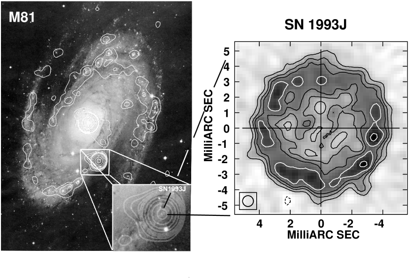
Figure 1.— Left panel: An optical image of the spiral galaxy M81 (Sandage 1961) with a VLA contour image overlaid and with SN 1993J prominent as the brightest radio source after the nucleus of the galaxy. Right panel: A composite VLBI image of SN 1993J at 8.4 GHz from three epochs at $t=2080$, 2525 and 2787 d (1998 December to 2000 November) all corrected for position shifts, scaled in flux density and radius to the values of the 2000 November data, and then combined (adopted from Paper III). The beam (FWHM, 0.70 mas) is shown at lower left. The contours are drawn at $-16$, 16, 32, 45.3, 64 and 90% of the peak brightness, and the background rms was 5.3% of the peak brightness. North is up and east to the left.

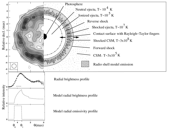
Figure 2.— Top panel: The left part of the composite VLBI image of SN 1993J from Figure 1. The outer overlayed circle shows the fit outer radius, $\theta_{\rm o}$, of the shell model with absorption in the center and indicates the expected location of the forward shock front, which is expanding into the circumstellar medium (CSM). The inner circle shows the fit inner radius, $\theta_{\rm i}$, of that shell model and indicates the expected location of the reverse shock front. The forward and reverse shock fronts travel in co-moving opposite directions (see arrows) from the contact discontinuity, or contact surface, where the ejecta hit the CSM. The location of the contact surface is shown by the dashed circle. Fingers expanding into the shocked CSM due to the contact surface being Rayleigh-Taylor unstable are also shown. The smaller dashed-dotted circle indicates the boundary between the colder, neutral ejecta and the hotter, ionized ejecta. Broad line emission is expected from the ionized ejecta up to the contact surface. The center of the circles is at the fit center position (see Paper I). Typical temperatures are also indicated. Second panel from top: The brightness profile of the composite image above, averaged over all p.a.’s, plotted as a function of angular radius, $\theta$. The resolution is 0.70 mas, and the plotted uncertainties are the standard errors of the bin values, derived from the number of beam areas within each bin and the larger of the standard deviation within that bin and the rms of the noise of the background brightness. The plotted values are correlated, especially at small radii, because they are less than 1 beamwidth apart. Also indicated is the corresponding radial profile of the projected best fit spherical shell model with uniform emissivity and an absorption disk in the center, convolved to the resolution of 0.70 mas. Third panel from top: The corresponding radial profile of the projected unconvolved shell model with absorption. Bottom panel: The radial profile of the volume emissivity of the shell (without absorption). The shell is limited by $\theta_{\rm o}$ and $\theta_{\rm i}$.

Figure 3.— The ratio $\theta_{\rm o}$/$\theta_{\rm i}$, which is a measure of the shell thickness, as a function of time. The data points are our measurements at times when the shell was sufficiently large for a thickness determination (from Paper II). The thin horizontal line from $t=996$ d to 2996 d gives the mean of $\theta_{\rm o}$/$\theta_{\rm i}$ = 1.29 for this time interval. The dotted line gives the prediction from hydrodynamic simulations.

Figure 4.— The angular outer radius, $\theta_{\rm o}$, of the SN 1993J shell model as a function of time since shock breakout. Taken from Paper II.

Figure 5.— The time derivatives of the angular radii of the outer ($\dot{\theta}_{\rm o}$, upper solid curve) and inner ($\dot{\theta}_{\rm i}$, lower solid curve) surfaces of the radio shell, the contact surface ($\dot{\theta}_{\rm c}$, curve with short dashes), and the mean between the outer surface and the contact surface ($\dot{\theta}_{\rm x}$, curve with dots). The thin curves with long dashes on both sides of the upper solid curve indicate the (asymmetric) standard error of 1 to 5% of $\dot{\theta}_{\rm o}$ as a function of time (see text).

Figure 6.— The observed expansion velocities from the width of the H$\alpha$ line from Table 1 as a function of time. The symbols represent the BVZI (blue velocity at zero intensity) values from the absorption trough of the line (filled square), and the BVZI (filled circle), BVHI (blue velocity at half intensity, filled triangle), RVZI (red velocity at zero intensity, open circle) and RVHI (red velocity at half intensity, open triangle) values, all from the emission line.

Figure 7.— As in Figure 6 but now showing only the BVZI H$\alpha$ values to which $D$$\dot{\theta}_{\rm x}$ (Mean) was fit to determine the distance, $D$. In addition the velocity curves, $D$$\dot{\theta}_{\rm o}$, $D$$\dot{\theta}_{\rm i}$, $D$$\dot{\theta}_{\rm c}$, and $D$$\dot{\theta}_{\rm x}$  are plotted (see Figure 5) for the best fit distance of $D=3.96$ Mpc.

Figure 8.— As in Figure 7 but now also with the BVZI values of the H$\beta$ emission line from Table 1.

Figure 9.— As in Figure 7, but now also with the RVZI values of the O[III] and Na I emission lines from Table 1.

Figure 10.— As in Figure 7, but now the velocity curves are plotted for a distance of 3.67 Mpc, which is the 1$\sigma$ lower limit of our distance estimate of $3.96\pm 0.29$ Mpc.

Figure 11.— As in Figure 7, but now the velocity curves are plotted for a distance of 4.25 Mpc, which is the 1$\sigma$ upper limit of our distance estimate of $3.96\pm 0.29$ Mpc.

References

- (1) Aaronson, M., Mould, J., & Huchra, J. 1980, ApJ, 237, 655
- (2) Baade, W. 1926, Astron. Nachr., 228, 359
- (3) Baron, E., et al. 1995, ApJ, 441, 170
- (4) Baron, E., Nugent, P. E., Branch, D., & Hauschildt, P. H. 2004, ApJ, 616, L91
- (5) Bartel, N. 1985 in Supernovae as Distance Indicators, Lecture Notes in Physics, ed. N. Bartel (Berlin: Springer Verlag), 221
- (6) Bartel, N., Rogers, A. E. E., Shapiro, I. I., Gorenstein, M. V., Gwinn, C. R., Marcaide, J. M., & Weiler, K. W. 1985, Nature, 318, 25
- (7) Bartel, N., et al. 1994, Nature, 386, 610
- (8) Bartel, N., et al. 2000, Science, 287, 112
- (9) Bartel, N., et al. 2002, ApJ, 581, 404 (Paper II)
- (10) Bartel, N. & Bietenholz, M. F. 2003, ApJ, 591, 301
- (11) Bartel, N. & Bietenholz, M. F. 2005, in The 10th Anniversary Of The VLBA, ed. J. Romney & M. Reid (ASP San Francisco), 340, 293
- (12) Bartel, N. & Bietenholz, M. F. 2005, Adv. Sp. Res., 35, 1057
- (13)
- (14) Bietenholz, M. F., Bartel, N., & Rupen, M. P. 2000, ApJ, 532, 895
- (15) Bietenholz, M. F., Bartel, N., & Rupen, M. P. 2001, ApJ, 556, 770 (Paper I)
- (16) Bietenholz, M. F., Bartel, N., & Rupen, M. P. 2003, ApJ, 597, 374 (Paper III)
- (17) Bietenholz, M. F., Bartel, N., & Rupen, M. P. 2004a, ApJ, 615, 173
- (18) Bietenholz, M. F., Bartel, N., & Rupen, M. P. 2004b, Science, 304, 1947
- (19) Bietenholz, M. F., et al. 1996, ApJ, 457, 604
- (20) Blondin, J. M., & Ellison, D. C. 2001, ApJ, 560, 244
- (21) Bonanos, A. Z., et al. 2006, ApJ, 652, 313
- (22) Brunthaler, A., et al. 2005, Science, 307, 1440
- (23) Caldwell, N., Armandroff, T. E., Da Costa, G. S., & Seitzer, P. 1998, AJ, 115, 535
- (24) Chevalier, R. A. 1982a, ApJ, 258, 790
- (25) Chevalier, R. A. 1982b, ApJ, 259, 302
- (26) Chevalier, R. A., Blondin, J. M., & Emmering, R. T. 1992, ApJ, 392, 118
- (27) Chevalier, R. A., & Fransson, C. 1994, ApJ, 420,268
- (28) Clocchiatti, A., Wheeler, J. C., Barker, E. S., Filippenko, A. V., Matheson, T., & Liebert, J. W. 1995, ApJ, 446, 167
- (29) Deneault, E. A.-N., Clayton, C. C., & Heger, A. 2003, ApJ, 594, 312
- (30) Dessart, L. & Hillier, D. J. 2005, A&A, 439, 685
- (31) Dwarkadas, V. V. 2000, ApJ, 541, 418
- (32) Dwarkadas, V. V. & Chevalier, R. A. 1998, ApJ, 497, 807
- (33) Eastman, R. G. & Kirshner, R. P. 1989, ApJ, 347, 771
- (34) Eastman, R. G., Schmidt, B. P., & Kirshner, R. 1996, ApJ, 466, 911
- (35) Elmhamdi, A. et al. 2003, MNRAS, 338, 939
- (36) Filippenko, A. V., Matheson, T., & Barth, A. J. 1994, AJ, 108, 2220
- (37) Finn, R. A., Fesen, R. A., Darling, G. W., Thorstensen, J. R., & Worthey, G. S. 1995, AJ, 110, 300
- (38) Fransson, C. & Björnsson, C.-I. 1998, ApJ, 509, 861
- (39) Fransson, C., Lundqvist, P. & Chevalier, R. A. 1996, ApJ, 461, 993
- (40) Fransson, C., et al. 2005, ApJ, 622, 991
- (41) Freedman, W. L., et al. 1994, ApJ, 427, 628
- (42) Freedman, W. L., et al. 2001, ApJ, 553, 47
- (43) Gerardy, C. L., Fesen, R. A., Höflich, P, & Wheeler, J. C. 2000, AJ, 119, 2968
- (44) Gull, S. F. 1973, MNRAS, 161, 47
- (45) Hamuy, M., et al. 2001, ApJ, 558, 615
- (46) Herrnstein, J. R. et al. 1999, Nature, 400, 539
- (47) Höflich, P. 1995, ApJ, 440, 821
- (48) Höflich, P., Wheeler, J. C., Hines, D. C., & Trammell, S. R. 1996, ApJ, 459, 307
- (49) Houck J. C., & Fransson, C. 1996, ApJ, 456, 811
- (50) Huterer, D., Sasselov, D. D., & Schechter, P. L. 1995, AJ, 110, 2705
- (51) Jacoby, G. H., Ciardullo, R., Booth, J., & Ford, H. C. 1989, ApJ, 344, 704
- (52) Jun, B.-I., & Norman, M. L. 1996a, ApJ, 465, 800
- (53) Jun, B.-I., & Norman, M. L. 1996b, ApJ, 472, 245
- (54) Karachentsev, I. D., et al. 2002, A&A, 383, 125
- (55) Karachentsev, I. D., et al. 2003, A&A, 398, 479
- (56) Kirshner, R. P. & Kwan, J. 1974, ApJ, 193, 27
- (57) Leonard, D. C., et al. 2002, PASP, 114, 35
- (58) Leonard, D. C., Kanbur, S. M., Ngeow, C. C., & Tanvir, N. R. 2003, ApJ, 594, 247
- (59) Lewis, J. M., et al. 1994, MNRAS, 266, L29
- (60) Lundqvist, P. & Fransson, C. 1988, A&A, 192, 221
- (61) Macri, L. M., Stanek, K. Z., Bersier, D., Greenhill, J. J., & Reid, M. J. 2006, ApJ, 652, 1133
- (62) Maoz, E., Newman, J., Ferrarese, L., Davis, M., Freedman, W. L., Madore, B. F., Stedson, P. B., & Zepf, S. 1999, Nature, 401, 351
- (63) Marcaide J. M., et al. 1997, ApJ, 486, L31
- (64) Matheson, T., et al. 2000a, AJ, 120, 1487
- (65) Matheson, T., Filippenko, A. V., Ho, L. C., Barth, A. J., & Leonard, D. C. 2000b, AJ, 120, 1499
- (66) Maund, J. R., Smartt, S. J., Kudritzki, R. P., Podsiadlowski, P., & Gilmore, G. F. 2004, Nature, 427, 129
- (67) Mioduszewski, A. J., Dwarkadas, V. V., & Ball, L. 2001, ApJ, 562, 869
- (68) Newman, J. A., Ferrarese, L., Stetson, P. B., Maoz, E., Zepf, E., Davis, M., Freedman, W. L., & Madore, B. F. 2001, ApJ, 553, 562.
- (69) Patat, F., Chugai, N., & Mazzali, P. A. 1995, A&A, 299, 715
- (70) Podsiadlowski, Ph., Hsu, J. J. L., Joss, P. C., & Ross, R. R. 1993, Nature, 364, 509
- (71) Prabhu, T. P., et al. 1995, A&A, 295, 403
- (72) Ripero, J., & Garcia, F. 1993, IAU Circ., 5731
- (73) Sandage, A. 1961 in The Hubble Atlas of Galaxies, Carnegie Institution of Washington, 618, 19
- (74) Sandage, A., Tammann, G. A., Saha, A., Reindl, B., Machetto. D, & Panagia, N. 2006, ApJ, 653, 843
- (75) Schmidt, B. P., et al. 1993, Nature, 364, 600
- (76) Shigeyama, T., Suzuki, T., Kumagai, S., Nomoto, K., Saio, H., & Yamaoka, H. 1994, ApJ, 420, 341
- (77) Spyromilio, J. 1994, MNRAS, 266, L61
- (78) Suzuki, T., & Nomoto, K. 1995, ApJ, 455, 658
- (79) Trammell, S. R., Hines, D. C., & Wheeler, J. C. 1993, ApJ, 414, L21
- (80) Tran, H. D., Filippenko, A. V., Schmidt, G. D., Bjorkman, K. S., Jannuzi, B. T., & Smith, P. S. 1997, PASP, 109, 489
- (81) van Leeuwen, F., Feast, M. W., Whitelock, P. A., & Laney, C. D. 2007, MNRAS, in press, astro-ph 0705.1592
- (82) Wesselink, A. J. 1946, Bulletin of the Astronomical Institutes of the Netherlands, 10, 91
- (83) Wheeler, J. C., et al. 1993, ApJ, 417, L71
- (84) Zimmermann, H.-U. & Aschenbach, B. 2003, A&A, 406, 969