Magnetic susceptibility of the two-dimensional Hubbard model
using a power series for the hopping constant

Abstract

The magnetic susceptibility of the two-dimensional repulsive Hubbard model with nearest-neighbor hopping is investigated using the diagram technique developed for the case of strong correlations. In this technique a power series in the hopping constant is used. At half-filling the calculated zero-frequency susceptibility and the square of the site spin reproduce adequately results of Monte Carlo simulations. Also in agreement with numerical simulations no evidence of ferromagnetic correlations was found in the considered range of electron concentrations $0.8\lesssim\bar{n}\lesssim 1.2$ for the repulsion parameters $8|t|\leq U\leq 16|t|$. However, for larger $U/|t|$ and $|1-\bar{n}|\approx 0.2$ the nearest neighbor correlations become ferromagnetic. For $\bar{n}\lesssim 0.94$ and $\bar{n}\gtrsim 1.06$ the imaginary part of the real-frequency susceptibility becomes incommensurate for small frequencies. The incommensurability parameter grows with departure from half-filling and decreases with increasing the frequency. This behavior of the susceptibility can explain the observed low-frequency incommensurate response observed in normal-state lanthanum cuprates.

I Introduction

The Hubbard modelHubbard is thought to be appropriate to describe the main features of electron correlations in narrow energy bands, leading to collective effects such as magnetism and metal-insulator transition. It has been often used to describe real materials exhibiting these phenomena (see, e.g., Refs. Izyumov, , Ovchinnikov, , and references therein).

In more than one dimension, the model is not exactly solvable and a variety of numerical and analytical approximate methods was used for its study. Among others there are Monte Carlo simulations,Hirsch ; Moreo different cluster methods,Maier the composite operator formalism,Mancini the generating functional approach,Izyumov05 Green’s function decoupling schemes,Irkhin and variational approaches.Seibold Along with these methods various versions of the diagram technique Izyumov ; Ovchinnikov ; Zaitsev ; Vladimir ; Pairault ; Sherman06 have been used for the investigation of the model. In the case of strong electron correlations when the ratio of the hopping constant $t$ to the on-site repulsion $U$ is a small parameter the use of the diagram technique based on the series expansion in this parameter is quite reasonable.

In the present work we use the diagram technique of Refs. Vladimir, and Sherman06, for investigating the magnetic susceptibility of the one-band two-dimensional repulsive Hubbard model with nearest-neighbor hopping in the case of strong electron correlations. In this version of the diagram technique terms of the power expansion are expressed through cumulants of creation and annihilation electron operators. The considered model possesses the electron-hole symmetry and results obtained for electron concentrations $\bar{n}<1$ are replicated for $\bar{n}>1$. Therefore in the following discussion we shall restrict our consideration to the former region of concentrations.

We found that at half-filling the calculated temperature dependence of the zero-frequency susceptibility reproduces adequately key features of results of Monte Carlo simulations.Hirsch The uniform susceptibility tends to a finite value for vanishing temperature. The staggered susceptibility diverges with decreasing temperature which signals the establishment of the long-range antiferromagnetic order. The transition temperature $T_{0}$ is finite which indicates the violation of the Mermin-Wagner theorem.Mermin However, the transition temperature is always lower than the analogous temperature in the random phase approximation (RPA). Besides, the transition temperature decreases with decreasing the ratio $|t|/U$ of the hopping constant and the on-site repulsion, i.e. the violation of the Mermin-Wagner theorem becomes less pronounced on enforcing the condition for which the approximation was developed. For small ratios $|t|/U$ the calculated square of the site spin differs by less than 10% from the data of Monte Carlo simulations. Also in agreement with Monte Carlo results we found no evidence of ferromagnetic correlations in the considered range of electron concentrations $0.8\lesssim\bar{n}\lesssim 1.2$ for the repulsion parameters $8|t|\leq U\leq 16|t|$. However, for larger $U/|t|$ and $|1-\bar{n}|\approx 0.2$ the nearest neighbor correlations become ferromagnetic. In the case $U=8|t|$ for $0.94\lesssim\bar{n}\lesssim 1.06$ the zero-frequency susceptibility and the imaginary part of the susceptibility for low real frequencies are peaked at the antiferromagnetic wave vector $(\pi,\pi)$. For smaller and larger concentrations these susceptibilities become incommensurate – momenta of their maxima deviate from $(\pi,\pi)$ – and the incommensurability parameter, i.e. the distance between $(\pi,\pi)$ and the wave vector of the susceptibility maximum, grows with departure from half-filling. With increasing the frequency the incommensurability parameter decreases and finally vanishes. This behavior of the strongly correlated system resembles the incommensurate magnetic response observed in the normal-state lanthanum cupratesYamada and can be used for its explanation.

Main formulas used in the calculations are given in the following section. The discussion of the obtained results and their comparison with data of Monte Carlo simulations are carried out in Sec. III. Concluding remarks are presented in Sec. IV. A relation between the longitudinal and transversal spin Green’s function is checked in the Appendix.

Figure 1: The diagram equation for $D({\bf k},i\omega_{\nu})$.

II Main formulas

The Hubbard model is described by the Hamiltonian

$$H=\sum_{\bf ll^{\prime}\sigma}t_{\bf ll^{\prime}}a^{\dagger}_{\bf l\sigma}a_{\bf l^{\prime}\sigma}+\frac{U}{2}\sum_{\bf l\sigma}n_{\bf l\sigma}n_{\bf l,-\sigma},$$ (1)

where $a^{\dagger}_{\bf l\sigma}$ and $a_{\bf l\sigma}$ are the electron creation and annihilation operators, ${\bf l}$ labels sites of the square plane lattice, $\sigma=\pm 1$ is the spin projection, $t_{\bf ll^{\prime}}$ and $U$ are hopping and on-site repulsion constants, and $n_{\bf l\sigma}=a^{\dagger}_{\bf l\sigma}a_{\bf l\sigma}$. Below we consider the case where only the constant $t$ for hopping between nearest neighbor sites is nonzero.

In the case of strong correlations, $U\gg|t|$, for calculating Green’s functions it is reasonable to use the expansion in powers of the hopping constant. In the diagram technique of Refs. Vladimir, and Sherman06, this expansion is expressed in terms of site cumulants of electron creation and annihilation operators. We use this technique for calculating the spin Green’s function

$$D({\bf l^{\prime}\tau^{\prime},l\tau})=\langle{\cal T}s^{\sigma}_{\bf l^{\prime}}(\tau^{\prime})s^{-\sigma}_{\bf l}(\tau)\rangle,$$ (2)

where $s^{\sigma}_{\bf l}=a^{\dagger}_{\bf l\sigma}a_{\bf l,-\sigma}$ is the spin operator, the angular brackets denote the statistical averaging with the Hamiltonian

$${\cal H}=H-\mu\sum_{\bf l\sigma}n_{\bf l\sigma},$$

$\mu$ is the chemical potential, ${\cal T}$ is the time-ordering operator which arranges other operators from right to left in ascending order of times $\tau$, and

$$a_{\bf l\sigma}(\tau)=\exp({\cal H}\tau)a_{\bf l\sigma}\exp(-{\cal H}\tau).$$

The structure elements of the used diagram technique are site cumulants and hopping constants which connect the cumulants. Vladimir ; Sherman06 In diagrams, we denote the hopping constants by single directed lines. Using the diagram technique it can be shown that Green’s function (2) satisfies the diagram equation plotted in Fig. 1. In this diagram, after the Fourier transformation over the space and time variables the dual line indicates the full electron Green’s function

$$G({\bf k},n)=-\frac{1}{2}\int_{-\beta}^{\beta}e^{i\omega_{n}\tau}\big{\langle}{\cal T}a_{\bf k}(\tau)a^{\dagger}_{\bf k}\big{\rangle}\,d\tau,$$

where ${\bf k}$ is the wave vector, the integer $n$ stands for the fermion Matsubara frequency $\omega_{n}=(2n+1)\pi T$ with the temperature $T$, and $\beta=T^{-1}$. The shaded circle in Fig. 1 is the sum of all four-leg diagrams, i.e. such diagrams in which starting from any leg one can reach any other leg moving along the hopping lines and cumulants. These diagrams can be separated into reducible and irreducible diagrams. In contrast to the latter, the reducible diagrams can be divided into two disconnected parts by cutting two hopping lines. The sum of all four-leg diagrams satisfies the Bethe-Salpeter equation shown in Fig. 2. Here the open circle indicates the sum of all irreducible four-leg diagrams. The hopping lines between the open and shaded circles are already renormalized here by the inclusion of all possible irreducible two-leg diagrams into these lines. These irreducible two-leg diagrams cannot be divided into two disconnected parts by cutting one hopping line.Sherman06 As a consequence, the hopping line in Fig. 2 is described by the equation

$$\Theta({\bf k},n)=t_{\bf k}+t_{\bf k}^{2}G({\bf k},n),$$ (3)

where in the considered model with nearest-neighbor hopping we have $t_{\bf k}=2t[\cos(k_{x})+\cos(k_{y})]$. The irreducible two-leg diagrams can also be inserted in the external lines of the four-leg

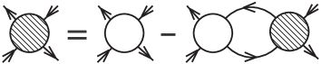
Figure 2: The Bethe-Salpeter equation for the sum of all four-leg diagrams.

diagrams in Fig. 1. To mark this renormalization we use dashed lines in that figure. Each of these lines introduces the multiplier $\Pi({\bf k},n)=\Theta({\bf k},n)/t_{\bf k}$ in the second term on the right-hand side of the equation in Fig. 1. Without the renormalization this multiplier reduces to unity.

As a result, the equations depicted in Figs. 1 and 2 read

$$D(p) = -N^{-1}T\sum_{p_{1}}G(p_{1})G(p+p_{1})$$ (4)

$$+ N^{-2}T^{2}\sum_{p_{1}p_{2}}\Pi(p_{1})\Pi(p_{2})\Pi(p+p_{1})\Pi(p+p_{2})$$

$$\times \Gamma(p_{1},p+p_{1},p+p_{2},p_{2}),$$

$$\Gamma(p_{1},p+p_{1},p+p_{2},p_{2})=\gamma(p_{1},p+p_{1},p+p_{2},p_{2})$$

$$\quad-N^{-1}T\sum_{p_{3}}\gamma(p_{1},p+p_{1},p+p_{3},p_{3})\Theta(p_{3})\Theta(p+p_{3})$$

$$\quad\times\Gamma(p_{3},p+p_{3},p+p_{2},p_{2}).$$ (5)

Here the combined indices $p=({\bf k},i\omega_{\nu})$ and $p_{j}=({\bf k}_{j},i\omega_{n_{j}})$ were introduced, $\omega_{\nu}=2\nu\pi T$ is the boson Matsubara frequency, $\Gamma(p_{1},p+p_{1},p+p_{2},p_{2})$ is the sum of all four-leg diagrams, $\gamma(p_{1},p+p_{1},p+p_{2},p_{2})$ is its irreducible subset, and $N$ is the number of sites.

In the following consideration we simplify the general equations (4) and (5) by neglecting the irreducible two-leg diagrams in the external and internal lines of the four-leg diagrams and by using the lowest-order irreducible four-leg diagram instead of $\gamma(p_{1},p+p_{1},p+p_{2},p_{2})$. This four-leg diagram is described by the second-order cumulant

$$K_{2}(\tau^{\prime},\tau,\tau^{\prime}_{1},\tau_{1}) = \langle{\cal T}\bar{a}_{\sigma}(\tau^{\prime})a_{-\sigma}(\tau)\bar{a}_{-\sigma}(\tau^{\prime}_{1})a_{\sigma}(\tau_{1})\rangle_{0}$$ (6)

$$+ K_{1}(\tau^{\prime},\tau_{1})K_{1}(\tau^{\prime}_{1},\tau),$$

where the subscript “0” of the angular bracket indicates that the averaging and time dependencies of the operators are determined by the site Hamiltonian

$$H_{\bf l}=\sum_{\sigma}[(U/2)n_{\bf l\sigma}n_{\bf l,-\sigma}-\mu n_{\bf l\sigma}],$$

$$\bar{a}_{\bf l\sigma}(\tau)=\exp(H_{\bf l}\tau)a^{\dagger}_{\bf l\sigma}\exp(-H_{\bf l}\tau),$$

and the first-order cumulant

$$K_{1}(\tau^{\prime},\tau)=\langle{\cal T}\bar{a}_{\sigma}(\tau^{\prime})a_{\sigma}(\tau)\rangle_{0}.$$

All operators in the cumulants belong to the same lattice site. Due to the translational symmetry of the problem the cumulants do not depend on the site index which is therefore omitted in the above equations. The expression for $K_{2}$ reads

$$K_{2}(n_{1},n_{1}+\nu,n_{2}+\nu,n_{2})=Z^{-1}\Big{\{}\beta\big{[}\delta_{\nu,0}e^{-E_{1}\beta}+Z^{-1}\delta_{n_{1},n_{2}}\big{(}e^{-2E_{1}\beta}-e^{-(E_{0}+E_{2})\beta}\big{)}\big{]}F(n_{1}+\nu)F(n_{2})$$

$$\quad+e^{-E_{0}\beta}Ug_{01}(n_{1}+\nu)g_{01}(n_{2})g_{02}(n_{1}+n_{2}+\nu)\big{[}g_{01}(n_{2}+\nu)+g_{01}(n_{1})\big{]}$$

$$\quad+e^{-E_{2}\beta}Ug_{12}(n_{1}+\nu)g_{12}(n_{2})g_{02}(n_{1}+n_{2}+\nu)\big{[}g_{12}(n_{2}+\nu)+g_{12}(n_{1})\big{]}$$

$$\quad-e^{-E_{1}\beta}\Big{[}F(n_{1}+\nu)g_{01}(n_{2})g_{01}(n_{2}+\nu)+F(n_{2})g_{01}(n_{1}+\nu)g_{01}(n_{1})$$

$$\quad+F(n_{2})g_{12}(n_{2}+\nu)\big{[}g_{12}(n_{1}+\nu)-g_{01}(n_{1})\big{]}+F(n_{1}+\nu)g_{12}(n_{1})\big{[}g_{12}(n_{2})-g_{01}(n_{2}+\nu)\big{]}\Big{]}\Big{\}},$$ (7)

where $E_{0}=0$, $E_{1}=-\mu$, and $E_{2}=U-2\mu$ are the eigenenergies of the site Hamiltonian $H_{\bf l}$, $Z=e^{-E_{0}\beta}+2e^{-E_{1}\beta}+e^{-E_{2}\beta}$ is the site partition function, $g_{ij}(n)=(i\omega_{n}+E_{i}-E_{j})^{-1}$, and $F(n)=g_{01}(n)-g_{12}(n)$.

It is worth noting that the used approximation retains the relation

$$D({\bf l^{\prime}\tau^{\prime},l\tau})=2D_{z}({\bf l^{\prime}\tau^{\prime},l\tau}),$$ (8)

where

$$D_{z}({\bf l^{\prime}\tau^{\prime},l\tau})=\langle{\cal T}s^{z}_{\bf l^{\prime}}(\tau^{\prime})s^{z}_{\bf l}(\tau)\rangle$$ (9)

and $s^{z}_{\bf l}=\frac{1}{2}\sum_{\sigma}\sigma a^{\dagger}_{\bf l\sigma}a_{\bf l\sigma}$ is the $z$ component of spin. Relation (8) follows from the invariance of Hamiltonian (1) with respect to rotations of the spin quantization axis.Fradkin The proof of Eq. (8) is given in the Appendix.

Equation (7) can be significantly simplified for the case of principal interest $U\gg T$. In this case, if $\mu$ satisfies the condition

$$\varepsilon<\mu<U-\varepsilon,$$ (10)

where $\varepsilon\gg T$, the exponent $e^{-\beta E_{1}}$ is much larger than $e^{-\beta E_{0}}$ and $e^{-\beta E_{2}}$. Therefore terms with $e^{-\beta E_{0}}$ and $e^{-\beta E_{2}}$ can be omitted in Eq. (7) which gives

$$K_{2}(n_{1},n_{1}+\nu,n_{2}+\nu,n_{2})=\frac{1}{2}\Big{\{}\beta\Big{(}\delta_{\nu,0}+\frac{1}{2}\delta_{n_{1},n_{2}}\Big{)}F(n_{1}+\nu)F(n_{2})$$

$$\quad-F(n_{1}+\nu)g_{01}(n_{2})g_{01}(n_{2}+\nu)-F(n_{2})g_{01}(n_{1}+\nu)g_{01}(n_{1})$$

$$\quad-F(n_{2})g_{12}(n_{2}+\nu)\big{[}g_{12}(n_{1}+\nu)-g_{01}(n_{1})\big{]}-F(n_{1}+\nu)g_{12}(n_{1})\big{[}g_{12}(n_{2})-g_{01}(n_{2}+\nu)\big{]}\Big{\}}.$$ (11)

From Eq. (5) with the kernel (11) it can be seen that $\Gamma$ does not depend on momenta ${\bf k}_{1}$ and ${\bf k}_{2}$. Since we neglected irreducible diagrams in the external lines, $\Pi(p)=1$ and in the second term on the right-hand side of Eq. (4) the summations over ${\bf k}_{1}$, ${\bf k}_{2}$, and $n_{2}$ can be carried out instantly. The resulting equation for $\Gamma^{\prime}_{\bf k}(\nu,n)=T\sum_{n^{\prime}}\Gamma_{\bf k}(n,n+\nu,n^{\prime}+\nu,n^{\prime})$ reads

$$\Gamma^{\prime}_{\bf k}(\nu,n) = \frac{1}{2}f_{\bf k}(\nu,n)\big{\{}2K^{\prime}_{2}(\nu,n)+\big{[}a_{2}(-\nu,\nu+n)-a_{1}(\nu+n)\beta\delta_{\nu,0}\big{]}tt_{\bf k}y_{1}({\bf k}\nu)+a_{1}(\nu+n)tt_{\bf k}y_{2}({\bf k}\nu)$$ (12)

$$+ a_{4}(-\nu,\nu+n)tt_{\bf k}y_{3}({\bf k}\nu)+a_{3}(-\nu,\nu+n)tt_{\bf k}y_{4}({\bf k}\nu)\big{\}},$$

where

$$K^{\prime}_{2}(\nu,n) = T\sum_{n^{\prime}}K_{2}(n,n+\nu,n^{\prime}+\nu,n^{\prime})$$ (13)

$$= \frac{1}{2}\bigg{\{}\bigg{[}\beta\delta_{\nu,0}+\frac{1}{2}a_{1}(n)\bigg{]}a_{1}(n+\nu)-a_{2}(-\nu,n+\nu)+\frac{1}{U-i\omega_{\nu}}a_{4}(-\nu,n+\nu)+a_{3}(-\nu,n+\nu)\bigg{\}},$$

$$f_{\bf k}(\nu,n)=\bigg{[}1+\frac{1}{4}F(n)F(\nu+n)tt_{\bf k}\bigg{]}^{-1},\quad y_{i}({\bf k}\nu)=T\sum_{n}a_{i}(\nu,n)\Gamma^{\prime}_{\bf k}(\nu,n),$$

(14)

$$a_{1}(n)=F(n),\quad a_{2}(\nu,n)=g_{01}(n)g_{01}(\nu+n),\quad a_{3}(\nu,n)=F(n)g_{12}(\nu+n),\quad a_{4}(\nu,n)=g_{12}(n)-g_{01}(\nu+n).$$

Multiplying Eq. (12) by $a_{i}(\nu,n)$ and summing over $n$ we obtain a system of four linear algebraic equations for $y_{i}$,

$$y_{i}=b_{i}+(c_{i2}-c_{i1}\beta\delta_{\nu,0})y_{1}+c_{i1}y_{2}+c_{i4}y_{3}+c_{i3}y_{4},$$ (15)

where

$$b_{i}=T\sum_{n}a_{i}(\nu,n)K^{\prime}_{2}(\nu,n)f_{\bf k}(\nu,n),\quad c_{ij}=tt_{\bf k}\frac{T}{2}\sum_{n}a_{i}(\nu,n)a_{j}(-\nu,\nu+n)f_{\bf k}(\nu,n).$$

System (15) can easily be solved. Thus, in the used approximation the Bethe-Salpeter equation (5) can be solved exactly. In notations (14) the second term on the right-hand side of Eq. (4) can be rewritten as

$$\bigg{(}\frac{T}{N}\bigg{)}^{2}\sum_{p_{1}p_{2}}\Gamma = \frac{T}{2}\bigg{\{}\big{[}\beta\delta_{\nu,0}(1-tt_{\bf k}y_{1})+tt_{\bf k}y_{2}\big{]}\sum_{n}f_{\bf k}(\nu,n)a_{1}(n+\nu)+\frac{1}{2}\sum_{n}f_{\bf k}(\nu,n)a_{1}(n)a_{1}(n+\nu)$$ (16)

$$- (1-tt_{\bf k}y_{1})\sum_{n}f_{\bf k}(\nu,n)a_{2}(-\nu,n+\nu)+\bigg{(}tt_{\bf k}y_{3}+\frac{1}{U-i\omega_{\nu}}\bigg{)}\sum_{n}f_{\bf k}(\nu,n)a_{4}(-\nu,n+\nu)$$

$$+ (1+tt_{\bf k}y_{4})\sum_{n}f_{\bf k}(\nu,n)a_{3}(-\nu,n+\nu)\bigg{\}}.$$

In subsequent calculations we shall use the Hubbard-I approximation Hubbard for the electron Green’s function in the first term on the right-hand side of Eq. (4). In the used diagram technique this approximation is obtained if in the Larkin equation the sum of all irreducible two-leg diagrams is substituted by the first-order cumulant.Vladimir ; Sherman06 Provided that condition (10) is fulfilled the electron Green’s function in the Hubbard-I approximation reads

$$G({\bf k}n)=\frac{i\omega_{n}+\mu-U/2}{(i\omega_{n}+\mu)(i\omega_{n}+\mu-U)-t_{\bf k}(i\omega_{n}+\mu-U/2)}.$$ (17)

III Magnetic susceptibility

From the Lehmann representationMahan it can be shown that $D_{z}({\bf k}\nu)$ has to be real, nonnegative,

$$D_{z}({\bf k}\nu)\geq 0$$ (18)

and symmetric, $D_{z}({\bf k}\nu)=D_{z}({\bf k},-\nu)$. In view of Eq. (8) analogous relations are fulfilled for $D({\bf k}\nu)$. However, we found that condition (18) is violated for $\nu=0$ and some momentum if the temperature drops below some critical value $T_{0}$ which depends on the ratio $|t|/U$ and on $\mu$. As the temperature $T_{0}$ is approached from above, $D({\bf k},0)$ tends to infinity which leads to the establishment of long-range spin correlations. Therefore, like in the RPA,Mahan ; Izyumov90 we interpret this behavior of Green’s function as a transition to a long-range order. Near half-filling the highest temperature $T_{0}$ occurs for the antiferromagnetic momentum $(\pi,\pi)$. Thus, near half-filling the system exhibits transition to the state with the long-range antiferromagnetic order.

In our calculations $T_{0}$ is finite. Since we consider the two-dimensional model and the broken symmetry is continuous, this result is in contradiction to the Mermin-Wagner theoremMermin and shows that the used approximation somewhat overestimates the effect of the interaction. However, it is worth noting that the value of $T_{0}$ decreases with decreasing the ratio $|t|/U$, i.e. the violation of the Mermin-Wagner theorem becomes less pronounced on enforcing the condition for which the approximation was developed. Notice that other approximate methods, including RPAHirsch and cluster methods, Maier lead also to the violation of the Mermin-Wagner theorem. In the following calculations we consider only the region $T>T_{0}$.

It was also found that for $\nu\neq 0$ condition (18) is violated in a small area of the Brillouin zone near the $\Gamma$ point. Green’s function is small for such momenta and small negative values of $D({\bf k}\nu)$ here are a consequence of the used approximations. It is worth noting that the renormalization of internal and external hopping lines should improve the behavior of $D({\bf k}\nu)$ in this region.

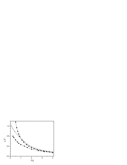
Figure 3: The zero-frequency magnetic susceptibility at ${\bf k}=0$ vs. temperature at half-filling and $t=-U/4$. Filled squares, filled and open circles are results of the Monte Carlo simulations, Hirsch random phase approximation, and our calculations, respectively.

To check the used approximation we shall compare our calculated results with data of Monte Carlo simulationsHirsch on the temperature dependence of the zero-frequency susceptibility at half-filling and on the square of the site spin $\langle{\bf S}^{2}\rangle$. In the usual definitionMahan the susceptibility $\chi({\bf k}\nu)$ differs from $D({\bf k}\nu)$ only in a constant multiplier. For convenience in comparison with results of Ref. Hirsch, in this work we set

$$\chi({\bf k}\nu)=D({\bf k}\nu).$$ (19)

The square of the site spin is given by the relation

$$\langle{\bf S}^{2}\rangle=\frac{3}{2}\frac{T}{N}\sum_{\bf k\nu}D({\bf k}\nu),$$ (20)

where Eq. (8) is taken into account.

The calculated zero-frequency magnetic susceptibility for ${\bf k}=0$ and half-filling is shown in Fig. 3. Results obtained in Monte Carlo simulationsHirsch and in the RPA are also shown here for comparison. The RPA results are described by the equationsMahan

$$\chi_{\rm RPA}({\bf k})=\frac{2\chi_{0}({\bf k})}{1-U\chi_{0}({\bf k})},$$

(21)

$$\chi_{0}({\bf k})=-\frac{1}{N}\sum_{\bf k^{\prime}}\frac{f(t_{\bf k^{\prime}}-\mu)-f(t_{\bf k^{\prime}+k}-\mu)}{t_{\bf k^{\prime}}-t_{\bf k^{\prime}+k}},$$

where $f(E)=[\exp(E\beta)+1]^{-1}$. Notice that to use the same scale for the susceptibility as in Ref. Hirsch, our calculated values (19) in Figs. 3 and 4 were multiplied by the factor 2. Also it should be mentioned that for $T>2|t|=U/2$ we violate condition (10); however, the calculated high-temperature susceptibility is in reasonable agreement with the Monte Carlo data. It deserves attention that in contrast to the RPA susceptibility which diverges for low temperatures the susceptibility in our approach tends to a finite value as it must.

The staggered magnetic susceptibility $\chi_{M}$ is shown in Fig. 4.

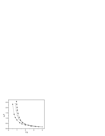
Figure 4: The zero-frequency magnetic susceptibility at ${\bf k}=(\pi,\pi)$ vs. temperature at half-filling and $t=-U/4$. Filled squares, filled and open circles are results of the Monte Carlo simulations, Hirsch random phase approximation, and our calculations, respectively.

As mentioned above, in the used approximation as the temperature approaches $T_{0}$ from above, $\chi_{M}$ tends to infinity which signals the establishment of the long-range antiferromagnetic order. For parameters of Fig. 4 $T_{0}\approx 0.64|t|$. The transition temperature $T_{0}$ is finite; however, for the considered range of parameters $4|t|\leq U\leq 16|t|$ it is always lower than the respective temperature in the RPA. Accordingly our calculated values of $\chi_{M}$ in Fig. 4 are closer to the Monte Carlo data than the RPA results.

The temperature variation of the square of the site spin, Eq. (20), is shown in Fig. 5 together with the data of Monte Carlo simulations.Hirsch

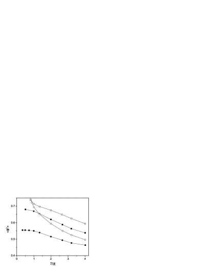
Figure 5: The square of the site spin $\langle{\bf S}^{2}\rangle$ vs. temperature at half-filling. Filled symbols are data of Monte Carlo simulations, Hirsch open symbols are our results. Squares and circles correspond to the cases $t=-U/8$ and $t=-U/4$, respectively.

As might be expected, the results for the smaller ratio $|t|/U$ more closely reproduce the data of numerical simulations. For $t=-U/8$ our calculations replicate the Monte Carlo data for $T\gtrsim|t|$ and the difference between the two series of results is less than 10 percent. This difference is at least partly connected with the simplification made above when irreducible two-leg diagrams were dropped from internal and external lines of the four-leg diagrams. The difference becomes even smaller if in accord with the Mermin-Wagner theorem $T_{0}$ is set as the zero of the temperature scale and our calculated curve is offset by this temperature to the left. On approaching $T_{0}$ our approximation becomes inapplicable for calculating $\langle{\bf S}^{2}\rangle$ – it starts to grow rapidly and exceeds the maximum value $\frac{3}{4}$.

The concentration dependence of $\langle{\bf S}^{2}\rangle$ near half-filling is shown in Fig. 6. The range of the electron concentration $\bar{n}=\sum_{\sigma}\langle n_{\bf l\sigma}\rangle$ which corresponds to the chemical potential shown in this figure spans approximately $0.8-1.2$ for $t=-U/8$. As would be expected, $\langle{\bf S}^{2}\rangle$ decreases rapidly with the departure from half-filling.

The momentum dependence of the zero-frequency susceptibility at half-filling and its variation with temperature are shown in Fig. 7. At half-filling the susceptibility is peaked at the antiferromagnetic wave vector $(\pi,\pi)$. For temperatures which are only slightly higher than $T_{0}$ the peak intensity is large [Fig. 7 (a)] which leads to a slow decrease of spin correlations with distance and long correlation lengths (see below). With increasing temperature the peak intensity of the susceptibility decreases rapidly [Fig. 7 (b) and (c)] which results in a substantial reduction of the correlation length. In this case for distances of several lattice periods the spin correlations are small, nevertheless they remain antiferromagnetic.

The situation is changed with the departure from half-filling. The zero-frequency susceptibility for different electron concentrations is shown in Fig. 8. The values of the concentration which correspond to parts (a) to (c) are $\bar{n}\approx 0.94$, 0.88, and 0.81, respectively. Notice the rapid decrease of the peak intensity of the susceptibility with doping [cf. parts (a) in this and the previous figure]. Starting from $\bar{n}\approx 0.94$ the susceptibility becomes incommensurate – the maximum value of the susceptibility is not located at $(\pi,\pi)$ – and the incommensurability parameter, i.e. the distance between $(\pi,\pi)$ and the wave vector of the susceptibility maximum, grows with departure from half-filling. It is interesting to notice that for $\bar{n}<1$ the zero-frequency susceptibility diverges when the temperature approaches some critical temperature in the same manner as it does at half-filling. For $t=-U/8$ and $0.94\lesssim\bar{n}\leq 1$ the divergence first occurs at $(\pi,\pi)$, while for smaller electron concentrations it appears at incommensurate wave vectors. For $\bar{n}<1$ the value of the critical temperature is less than $T_{0}$ – the temperature at which the transition to the long-range order occurs at half-filling. The critical temperature decreases with decreasing $\bar{n}$. If in accord with the Mermin-Wagner theorem we identify $T_{0}$ with zero temperature we have to conclude that for $\bar{n}<1$ the system undergoes a virtual transition at negative temperatures, while for $T\geq 0$ it is governed by short-range order. In view of the particle-hole symmetry analogous conclusions can be made for $\bar{n}>1$.

Figure 6: The square of the site spin $\langle{\bf S}^{2}\rangle$ vs. the chemical potential for $t=-U/8$ and $T=|t|$.

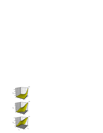
Figure 7: (Color online) The zero-frequency magnetic susceptibility at half-filling for $t=-U/8$ in a quadrant of the Brillouin zone. (a) $T=0.06U$, (b) $T=0.1U$, and (c) $T=0.2U$.

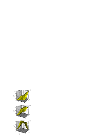
Figure 8: (Color online) The zero-frequency magnetic susceptibility for $t=-U/8$ and $T=0.06U$ in a quadrant of the Brillouin zone. (a) $\mu=0.2U$, (b) $\mu=0.15U$, and (c) $\mu=0.1U$.

Figure 9: (a) The momentum dependence of $\chi^{\prime\prime}({\bf k}\omega)$ along the edge [solid line, ${\bf k}=(\pi,\kappa)$] and diagonal [dashed line, ${\bf k}=(\kappa,\kappa)$] of the Brillouin zone for $t=-0.11U$, $\omega=0.002U$ and $\bar{n}\approx 0.88$). (b) The momentum dependence of $\chi^{\prime\prime}({\bf k}\omega)$ along the zone edge for $\bar{n}\approx 0.88$ (solid line), $\bar{n}\approx 0.94$ (dashed line), and $\bar{n}=1$ (dash-dotted line). $t=-0.11U$ and $\omega=0.002U$. (c) The dispersion of maxima in $\chi^{\prime\prime}({\bf k}\omega)$ along the zone edge for $t=-0.11U$ and $\bar{n}\approx 0.88$.

Analyzing equations of the previous section it can be seen that the momentum dependence of the zero-frequency susceptibility is mainly determined by the multiplier $y_{1}({\bf k},\nu=0)$ in the first term on the right-hand side of Eq. (16). At half-filling the susceptibility is commensurate, since this term is peaked at $(\pi,\pi)$ and diverges at this momentum when $T\rightarrow+T_{0}$, as the determinant of the system (15) vanishes. At departure from half-filling the behavior of $y_{1}$ is governed by the term $b_{1}$ in this system. The term contains the sum

$$T\sum_{n}a^{2}_{1}(0,n)f_{\bf k}(0,n)=T\sum_{n}F^{2}(n)\bigg{[}1+\frac{1}{4}tt_{\bf k}F^{2}(n)\bigg{]}^{-1},$$ (22)

where $F(n)=-U[(i\omega_{n}+\mu)(i\omega_{n}+\mu-U)]^{-1}$. For half-filling the sum has a maximum at $(\pi,\pi)$, however with departure from half-filling the maximum shifts from $(\pi,\pi)$ and the susceptibility becomes incommensurate.

Together with the zero-frequency susceptibility the imaginary part of the real-frequency susceptibility,

$$\chi^{\prime\prime}({\bf k}\omega)={\rm Im}\,D({\bf k},\omega+i\eta),\quad\eta\rightarrow+0,$$ (23)

becomes also incommensurate. This quantity is of special interest, because it determines the dynamic structure factor measured in neutron scattering experiments.Kastner To carry out the analytic continuation of $D({\bf k}\nu)$ to the real frequency axis an algorithm Vidberg based on the use of Padé approximants can be applied. In this calculation 300 values of $D({\bf k}\nu)$ at equally spaced imaginary frequencies in the upper half-plane were used. The obtained dependencies of the susceptibility on the momentum for a fixed transfer frequency $\omega$ and the dispersion of low-frequency maxima in $\chi^{\prime\prime}$ are shown in Fig. 9. The susceptibility is shown in the first Brillouin zone and can be extended to the second zone by reflection with respect to the right $y$ axis. As seen from Figs. 9 (a) and (b), with departure from half-filling $\chi^{\prime\prime}({\bf k}\omega)$ becomes incommensurate and the incommensurability parameter grows with increasing $1-\bar{n}$.

This behavior of the susceptibility $\chi^{\prime\prime}({\bf k}\omega)$ in the Hubbard model resembles the low-frequency incommensurate magnetic response observed by inelastic neutron scattering in lanthanum cuprates.Yamada In these crystals, the incommensurability is observed both in the normal and superconducting states. For small transfer frequencies $\omega$ the maxima of the susceptibility are located on the edge of the Brillouin zone. For the parameters of Fig. 9 (a) our calculated susceptibility is also peaked on the zone edge. However, for other parameters the susceptibility on the diagonal may be comparable to that on the zone edge. This uncertainty in the position of the susceptibility maxima may be connected with errors introduced in the calculation results by the procedure of analytic continuation to real frequencies.

In experiment, for small $\omega$ the incommensurability parameter grows with the hole concentration $1-\bar{n}$ in the range $0.04\lesssim 1-\bar{n}\lesssim 0.12$ and saturates for its larger values. This behavior of the incommensurability parameter is reproduced in our calculations [see Fig. 9 (b)] and its values are close to those observed experimentally. For a fixed hole concentration the incommensurability parameter decreases with increasing $\omega$ and at some frequency $\omega_{r}$ the incommensurability disappears and the susceptibility $\chi^{\prime\prime}({\bf k}\omega)$ appears to be peaked at the antiferromagnetic momentum.Tranquada The same behavior is observed in the Hubbard model [see Fig. 9 (c)]. In lanthanum cuprates for the hole concentrations $1-\bar{n}\approx 0.12$ the frequency $\omega_{r}\approx 50$ meV. In Fig. 9 (c) we chose parameters so that $\omega_{r}$ was close to this value (for the superexchange constant $J=4t^{2}/U\approx 0.15$ eV and $t=-0.11U$ we find $U=3.1$ eV, $t=0.34$ eV, and $\omega_{r}=44$ meV). Notice that like in experiment $\omega_{r}$ decreases with decreasing $1-\bar{n}$.

A similar incommensurability is observed in YBa₂Cu₃O_7-y; Arai however, in this case due to a larger superconducting temperature and gap the magnetic incommensurability is usually observed in the superconducting state and the low-frequency part of the susceptibility is suppressed. As follows from the above discussion, in the Hubbard model the magnetic incommensurability is a property of strong electron correlations. The similarity of the mentioned experimental and calculated results gives ground to consider these strong correlations as a possible mechanism of the low-frequency incommensurability observed in experiment. A similar mechanism was observed for the related $t$-$J$ model in Ref. Sherman05, .

In experiment,Tranquada ; Arai for frequencies $\omega>\omega_{r}$ the susceptibility $\chi^{\prime\prime}({\bf k}\omega)$ becomes again incommensurate such that the dispersion of maxima in $\chi^{\prime\prime}({\bf k}\omega)$ resembles a sandglass. The most frequently used interpretations of this dispersion are based on the picture of itinerant electrons with the susceptibility calculated in the RPALiu and on the stripe picture.Tranquada ; Seibold06 In Ref. Sherman05, the sandglass dispersion was obtained in the $t$-$J$ model in the regime of strong electron correlations without the supposition of the existence of stripes. In this latter work the part of the sandglass dispersion for $\omega>\omega_{r}$ was related to the dispersion of excitations of localized spins. Similar notion was earlier suggested in Ref. Barzykin, . In our present calculations we did not obtain this upper part of the dispersion, since the used approximation does not describe the appearance of localized spins. A typical example of the frequency dependence of the susceptibility $\chi^{\prime\prime}({\bf k}\omega)$ which up to the multiplier $\pi^{-1}$ coincides with the spin spectral function is shown in Fig. 10.

Figure 10: The susceptibility $\chi^{\prime\prime}({\bf k}\omega)$ for ${\bf k}=(\pi,\pi)$, $t=-U/8$, $T=0.06U$, and $\mu=0.2U$ ($\bar{n}\approx 0.94$).

The susceptibility usually contains several maxima one of which is located at $\omega\ll U$, while others are placed at frequencies of the order of $U$. Since the localized spin excitations have frequencies in the range $0\leq\omega\lesssim 2J$ where $J=4t^{2}/U\ll U$, the former maximum could be taken as a signal for such excitation. However, the intensity of the maximum usually grows with temperature and with departure from half-filling. This indicates that the maximum is more likely due to a bound electron-hole state in which both components belong to the same Hubbard subband, while in the high-frequency maxima the components belong to different subbands.

In connection with the Nagaoka theoremNagaoka it is of interest to investigate the tendency towards the establishment of the ferromagnetic ordering with departure from half-filling. For a finite $U$ this problem was investigated by different analytical methodsHirsch ; Izyumov90 ; Penn ; Kubo and by Monte Carlo simulations.Hirsch Our results for the spin-spin correlator,

$$\langle s^{+}_{\bf L}s^{-}_{\bf 0}\rangle=\frac{T}{N}\sum_{\bf k\nu}\cos({\bf kL})D({\bf k}\nu),$$ (24)

as a function of the distance $L_{x}$ between spins are shown in Fig. 11 for different parameters.

Figure 11: The spin-spin correlator $\langle s^{+}_{\bf L}s^{-}_{\bf 0}\rangle$ for ${\bf L}=(L_{x},0)$ and $t=-U/8$. (a) $T=0.06U$, $\mu=0.5U$, (b) $T=0.125U$, $\mu=0.5U$, and (c) $T=0.06U$, $\mu=0.1U$ ($\bar{n}\approx 0.81$). Insets in (b) and (c) demonstrate the same data as in the main plots in a larger scale.

Figure 11 (a) demonstrates the short-range antiferromagnetic order at half-filling for a temperature which is slightly above $T_{0}$ (as discussed above in connection with Fig. 5, for such temperatures the value of $\langle s^{+}_{\bf 0}s^{-}_{\bf 0}\rangle$ is somewhat overestimated by the used approximation). Figure 11 (b) corresponds also to half-filling to somewhat higher temperature. In this case the correlations are still antiferromagnetic though they are characterized by a correlation length which is much shorter than that in Fig. 11 (a). We have found that the correlation length diverges when $T\rightarrow T_{0}$ which indicates the transition to the long-range antiferromagnetic order. Similar weak antiferromagnetic correlations were also obtained for moderate departures from half-filling. Figure 11 (c) corresponds to the lowest filling $\bar{n}\approx 0.81$ which is allowed by condition (10) for the given ratio $U/|t|$. According to the mean-field theoryHirsch and the generalized RPA Izyumov90 in this case the system has a ferromagnetic ground state. As seen from Fig. 11 (c), our calculated spin-spin correlations are still antiferromagnetic even for nearest neighbor spins. This result is in agreement with Monte Carlo simulationsHirsch carried out for the same parameters. Analogous result was also obtained for $U=16|t|$. However, a tendency for the establishment of ferromagnetic correlations can also be seen from the comparison of Figs. 11 (a) and (c) – the antiferromagnetic spin correlation on nearest neighbor sites becomes smaller with doping. For larger ratios of $U/|t|$ we can ascertain that the correlation changes sign and becomes ferromagnetic. In particular, it happens at $U/|t|=25$ and $\bar{n}\approx 0.77$. For these parameters condition (10) is still fulfilled.

IV Concluding remarks

In this article we investigated the magnetic susceptibility of the two-dimensional repulsive Hubbard model using the diagram technique developed for the case of strong electron correlations. In this technique the power series in the hopping constant is used. At half-filling the calculated temperature dependence of the zero-frequency susceptibility reproduces adequately key features of results of Monte Carlo simulations. The uniform susceptibility tends to a finite value for vanishing temperature. The staggered susceptibility diverges with decreasing temperature which signals the establishment of the long-range antiferromagnetic order. The transition temperature is finite which indicates the violation of the Mermin-Wagner theorem. However, the transition temperature is always lower than the analogous temperature in the RPA. Besides, the transition temperature decreases with the decrease of the ratio $|t|/U$ of the hopping constant and the on-site repulsion, i.e. the violation of the Mermin-Wagner theorem becomes less pronounced on enforcing the condition for which the approximation was developed. For small ratios $|t|/U$ the calculated square of the site spin differs by less than 10 percent from the data of Monte Carlo simulations. Also in agreement with Monte Carlo results we found no evidence of ferromagnetic correlations in the considered range of electron concentrations $0.8\lesssim\bar{n}\lesssim 1.2$ for the repulsion parameters $8|t|\leq U\leq 16|t|$. However, for larger $U/|t|$ and $|1-\bar{n}|\approx 0.2$ the nearest neighbor correlations become ferromagnetic. In the case $U=8|t|$ for $0.94\lesssim\bar{n}\lesssim 1.06$ the zero-frequency susceptibility and the imaginary part of the susceptibility for low real frequencies are peaked at the antiferromagnetic wave vector $(\pi,\pi)$. For smaller and larger concentrations these susceptibilities become incommensurate – momenta of their maxima are shifted from $(\pi,\pi)$ – and the incommensurability parameter, i.e. the distance between $(\pi,\pi)$ and the momentum of the maximum susceptibility, grows with departure from half-filling. With increasing the transfer frequency the incommensurability parameter decreases and finally vanishes. This behavior of the susceptibility in the strongly correlated system can explain the observed low-frequency incommensurate response in the normal state of lanthanum cuprates.

*

Appendix A

In this Appendix we prove the symmetry relation (8). In the zeroth order of the perturbation expansion for Green’s function (9) we find

$$D_{z}^{(0)}({\bf l^{\prime}\tau^{\prime},l\tau}) = \frac{1}{4}\sum_{\sigma\sigma^{\prime}}\sigma\sigma^{\prime}\Big{[}K^{\prime}_{2}(\tau^{\prime}\sigma^{\prime},\tau^{\prime}\sigma^{\prime},\tau\sigma,\tau\sigma)\delta_{\bf ll^{\prime}}+K_{1}(\tau^{\prime}\tau^{\prime})K_{1}(\tau\tau)-K_{1}(\tau^{\prime}\tau)K_{1}(\tau\tau^{\prime})\delta_{\bf ll^{\prime}}\delta_{\sigma\sigma^{\prime}}\Big{]}$$ (25)

$$= \frac{1}{2}\delta_{\bf ll^{\prime}}\Big{[}K^{\prime}_{2}(\tau^{\prime}\sigma,\tau^{\prime}\sigma,\tau\sigma,\tau\sigma)-K^{\prime}_{2}(\tau^{\prime}\sigma;\tau^{\prime}\sigma;\tau,-\sigma;\tau,-\sigma)-K_{1}(\tau^{\prime}\tau)K_{1}(\tau\tau^{\prime})\Big{]},$$

where we took into account that the first-order cumulant $K_{1}(\tau^{\prime}\tau)$ does not depend on $\sigma$ and therefore the second term in the sum vanishes. Up to the multiplier $\frac{1}{2}$ the last term on the right-hand side of Eq. (25) coincides with the respective term in the expansion for Green’s function (2). In the used diagram technique $K_{1}$ describes the bare electron Green’s function. Therefore that term contributes to the electron bubble shown in Fig. 1. From the higher-order terms it can be seen that inclusion of irreducible two-leg diagrams into the two bare Green’s functions of that term retains the one-to-one correspondence between terms of the bubble diagrams in $D$ and $D_{z}$ and the additional multiplier $\frac{1}{2}$ in the terms of $D_{z}$.

The second-order cumulant $K_{2}^{\prime}$ in Eq. (25) is defined as

$$K^{\prime}_{2}(\tau^{\prime}\sigma,\tau\sigma,\tau^{\prime}_{1}\sigma_{1},\tau_{1}\sigma_{1})=\langle{\cal T}\bar{a}_{\sigma}(\tau^{\prime})a_{\sigma}(\tau)\bar{a}_{\sigma_{1}}(\tau^{\prime}_{1})a_{\sigma_{1}}(\tau_{1})\rangle-K_{1}(\tau^{\prime},\tau)K_{1}(\tau^{\prime}_{1},\tau_{1})+K_{1}(\tau^{\prime},\tau_{1})K_{1}(\tau^{\prime}_{1},\tau)\delta_{\sigma\sigma_{1}}.$$ (26)

This definition is more general than Eq. (6) – the latter is obtained from Eq. (26) if we set $\sigma_{1}=-\sigma$ and interchange annihilation operators in $K_{2}$. After the Fourier transformation we find

$$K^{\prime}_{2}(n_{1}\sigma;n_{1}+\nu,\sigma;n_{2}+\nu,\sigma_{1};n_{2}\sigma_{1})=Z^{-1}\Big{\{}\beta\Big{[}\big{(}\delta_{\nu 0}\delta_{\sigma\sigma_{1}}-\delta_{n_{1}n_{2}}\big{)}e^{-E_{1}\beta}$$

$$\quad+Z^{-1}\big{(}\delta_{\nu 0}-\delta_{n_{1}n_{2}}\delta_{\sigma\sigma_{1}}\big{)}\Big{(}e^{-(E_{0}+E_{2})\beta}-e^{-2E_{1}\beta}\Big{)}\Big{]}F(n_{1}+\nu)F(n_{2})$$

$$\quad-\delta_{\sigma,-\sigma_{1}}e^{-E_{0}\beta}Ug_{01}(n_{1}+\nu)g_{01}(n_{2})g_{02}(n_{1}+n_{2}+\nu)\big{[}g_{01}(n_{2}+\nu)+g_{01}(n_{1})\big{]}$$

$$\quad-\delta_{\sigma,-\sigma_{1}}e^{-E_{2}\beta}Ug_{12}(n_{1}+\nu)g_{12}(n_{2})g_{02}(n_{1}+n_{2}+\nu)\big{[}g_{12}(n_{2}+\nu)+g_{12}(n_{1})\big{]}$$

$$\quad+\delta_{\sigma,-\sigma_{1}}e^{-E_{1}\beta}\Big{[}F(n_{1}+\nu)g_{01}(n_{2})g_{01}(n_{2}+\nu)+F(n_{2})g_{01}(n_{1}+\nu)g_{01}(n_{1})$$

$$\quad+F(n_{2})g_{12}(n_{2}+\nu)\big{[}g_{12}(n_{1}+\nu)-g_{01}(n_{1})\big{]}+F(n_{1}+\nu)g_{12}(n_{1})\big{[}g_{12}(n_{2})-g_{01}(n_{2}+\nu)\big{]}\Big{]}\Big{\}},$$ (27)

where the notations are the same as in Eq. (7). From these two equations it can be seen that

$$K_{2}(n_{1},n_{1}+\nu,n_{2}+\nu,n_{2})=K^{\prime}_{2}(n_{1}\sigma;n_{1}+\nu,\sigma;n_{2}+\nu,\sigma;n_{2}\sigma)-K^{\prime}_{2}(n_{1}\sigma;n_{1}+\nu,\sigma;n_{2}+\nu,-\sigma;n_{2},-\sigma)$$ (28)

and the analogous equation is fulfilled for the Fourier-transformed quantities. Thus, zeroth-order terms in the expansions for $D$ and $D_{z}$ coincide up to the factor $\frac{1}{2}$.

The next terms in the considered expansions for $D$ and $D_{z}$ contain two second-order cumulants and appear in the second order. These terms read

$$D^{(2)}({\bf l^{\prime}\tau^{\prime},l\tau}) = -\int\!\!\!\int_{0}^{\beta}d\tau_{1}d\tau_{2}t_{\bf ll^{\prime}}t_{\bf l^{\prime}l}K_{2}(\tau^{\prime},\tau^{\prime},\tau_{1},\tau_{2})K_{2}(\tau_{2},\tau_{1},\tau,\tau),$$ (29)

$$D_{z}^{(2)}({\bf l^{\prime}\tau^{\prime},l\tau}) = -\frac{1}{4}\sum_{\sigma\sigma^{\prime}\sigma_{1}}\int\!\!\!\int_{0}^{\beta}d\tau_{1}d\tau_{2}t_{\bf ll^{\prime}}t_{\bf l^{\prime}l}K^{\prime}_{2}(\tau^{\prime}\sigma^{\prime},\tau^{\prime}\sigma^{\prime},\tau_{1}\sigma_{1},\tau_{2}\sigma_{1})K^{\prime}_{2}(\tau_{2}\sigma_{1},\tau_{1}\sigma_{1},\tau\sigma,\tau\sigma).$$ (30)

Using twice relation (28) in Eq. (30) one can see that $D^{(2)}=2D^{(2)}_{z}$. Analogous equations for higher order terms can be proved in the same manner. Thus, relation (8) is fulfilled.

References

- (1) J. Hubbard, Proc. R. Soc. London, Ser. A 276, 238 (1963); M. C. Gutzwiller, Phys. Rev. Lett. 10, 159 (1963); J. Kanamori, Prog. Theor. Phys. 30, 275 (1963).
- (2) Yu. A. Izyumov and Yu. N. Skryabin, Statistical Mechanics of Magnetically Ordered Systems, (Consultants Bureau, New York, 1988).
- (3) S. G. Ovchinnikov and V. V. Valkov, Hubbard operators in the theory of strongly correlated electrons, (Imperial College Press, London, 2004).
- (4) J. E. Hirsch, Phys. Rev. B 31, 4403 (1985).
- (5) A. Moreo, S. Haas, A. W. Sandvik, and E. Dagotto, Phys. Rev. B 51, 12045 (1995); C. Gröber, R. Eder, and W. Hanke, Phys. Rev. B 62, 4336 (2000).
- (6) T. Maier, M. Jarrell, T. Pruschke, and M. H. Hettler, Rev. Modern Phys. 77, 1027 (2005); M. Aichhorn, E. Arrigoni, M. Potthoff, and W. Hanke, Phys. Rev. B 74, 024508 (2006); A.-M. S. Tremblay, B. Kyung, and D. Sénéchal, Fizika Nizkikh Temperatur 32, 561 (2006).
- (7) F. Mancini and A. Avella, Adv. Phys. 53, 537 (2004).
- (8) Yu. A. Izyumov, N. I. Chaschin, D. S. Alexeev, and F. Mancini, Eur. Phys. J. B 45, 69 (2005).
- (9) V. Yu. Irkhin and A. V. Zarubin, Phys. Rev. B 70, 035116 (2004).
- (10) G. Seibold, F. Becca, P. Rubin, and J. Lorenzana, Phys. Rev. B 69, 155113 (2004).
- (11) R. O. Zaitsev, ZhETF 70, 1100 (1976) [Sov. Phys. JETP 43, 574 (1976)].
- (12) M. I. Vladimir and V. A. Moskalenko, Teor. Mat. Fiz. 82, 428 (1990) [Theor. Math. Phys. 82, 301 (1990)]; W. Metzner, Phys. Rev. B 43, 8549 (1991).
- (13) S. Pairault, D. Sénéchal and A.-M. S. Tremblay, Eur. Phys. J. B 16, 85 (2000).
- (14) A. Sherman, Phys. Rev. B 73, 155105 (2006); 74, 035104 (2006).
- (15) N. D. Mermin, and H. Wagner, Phys. Rev. Lett. 17, 1133 (1966).
- (16) T. E. Mason, G. Aeppli, S. M. Hayden, A. P. Ramirez, and H. A. Mook, Phys. Rev. Lett. 71, 919 (1993); K. Yamada, C.H. Lee, K. Kurahashi, J. Wada, S. Wakimoto, S. Ueki, H. Kimura, Y. Endoh, S. Hosoya, G. Shirane, R.J. Birgeneau, M. Greven, M.A. Kastner, and Y.J. Kim, Phys. Rev. B 57, 6165 (1998).
- (17) E. Fradkin, Field Theories of Condensed Matter Systems, (Addison Wesley, New York, 1991).
- (18) G. D. Mahan, Many-Particle Physics, (Plenum Press, New York, 1981).
- (19) Yu. A. Izyumov and B. M. Letfulov, J. Phys.: Condens. Matter 2, 8905 (1990); Yu. A. Izyumov, B. M. Letfulov, and E. V. Shipitsyn, J. Phys.: Condens. Matter 4, 9955 (1992); 6, 5137 (1994).
- (20) M. A. Kastner, R. J. Birgeneau, G. Shirane, and Y. Endoh, Rev. Mod. Phys. 70, 897 (1998).
- (21) H. J. Vidberg and J. W. Serene, J. Low Temp. Phys. 29, 179 (1977); G. A. Baker, Jr. and P. Graves-Morris, Padé Approximants, (Addison-Wesley, London, 1981).
- (22) J. M. Tranquada, H. Woo, T. G. Perring, H. Goka, G. D. Gu, G. Xu, M. Fujita, and K. Yamada, Nature 429, 534 (2004).
- (23) M. Arai, T. Nishijima, Y. Endoh, T. Egami, S. Tajima, K. Tomimoto, Y. Shiohara, M. Takahashi, A. Garrett, and S. M. Bennington, Phys. Rev. Lett. 83, 608 (1999).
- (24) A. Sherman and M. Schreiber, Int. J. Modern Phys. B 19, 2145 (2005); 21, 669 (2007).
- (25) D. Z. Liu, Y. Zha, and K. Levin, Phys. Rev. Lett. 75, 4130 (1995); J. Brinckmann and P. A. Lee, Phys. Rev. Lett. 82, 2915 (1999); M. R. Norman, Phys. Rev. B 61, 14751 (2000).
- (26) M. Vojta, T. Vojta, R. K. Kaul, Phys. Rev. Lett. 97, 097001 (2006); G. Seibold and J. Lorenzana, Phys. Rev. B 73, 144515 (2006).
- (27) V. Barzykin and D. Pines, Phys. Rev. B 52, 13585 (1995).
- (28) Y. Nagaoka, Phys. Rev. 147, 392 (1966).
- (29) D. Penn, Phys. Rev. 142, 350 (1966).
- (30) K. Kubo, Progr. Theor. Phys. 64, 758 (1980).