Percolation and Loop Statistics in Complex Networks

Abstract

Complex networks display various types of percolation transitions. We show that the degree distribution and the degree-degree correlation alone are not sufficient to describe diverse percolation critical phenomena. This suggests that a genuine structural correlation is an essential ingredient in characterizing networks. As a signature of the correlation we investigate a scaling behavior in $M_{N}(h)$, the number of finite loops of size $h$, with respect to a network size $N$. We find that networks, whose degree distributions are not too broad, fall into two classes exhibiting $M_{N}(h)\sim(\mbox{constant})$ and $M_{N}(h)\sim(\ln N)^{\psi}$, respectively. This classification coincides with the one according to the percolation critical phenomena.

Introduction: Complex networks have been attracting much interest during the last decade. Structure, dynamics, and collective phenomena have become intriguing research subjects in network science Watts98 ; Albert02 ; Boccaletti06 ; Dorogovtsev07 . This work considers a structural correlation in complex networks. Discussing scaling behaviors of percolation transitions Callaway00 ; Cohen02 ; Lee04 ; Newman02 ; Vazquez03 ; Callaway01 ; Dorogovtsev01 ; JKim02 ; Krapivsky04 ; Noh07 , we will show that the structural correlation is an essential ingredient characterizing structural properties and collective phenomena of complex networks.

Structural inhomogeneity is one of the most salient features of complex networks. It is reflected on the broad degree distribution $p_{d}$ Albert02 . For the study of the inhomogeneity, the uncorrelated network has been considered. It is defined as an ensemble of networks specified only with a given degree distribution but random in any other aspect. This includes the Erdős-Rényi random graph Albert02 , the Molloy-Reed model Molloy95 , and the static model Goh01 ; Lee06 . It is revealed that the structural inhomogeneity encoded in $p_{d}$ leads to rich collective phenomena Dorogovtsev07 .

Many real-world networks display some structural correlations. The degree-degree (DD) correlation has been considered mostly Pastor-Satorras01 ; Newman02 . It refers to the correlation between degrees of nodes linked directly with an edge. Networks with a positive (negative) correlation are called to be assortative (disassortative). The DD correlation is represented with the two-point degree correlation function $p(d^{\prime},d)$ denoting the fraction of edges linking nodes of degree $d$ and $d^{\prime}$. With the DD correlation being incorporated, the randomly correlated (RC) network has been considered. It is defined as an ensemble of networks specified only with $p(d^{\prime},d)$, but again random in any other aspect Newman02 ; Vazquez03 ; Dorogovtsev04 .

Studying the RC network is a meaningful attempt to understand correlated networks. However, it remains unknown to what extent the RC network is a proper model for correlated networks. In this work we will show that there exists a class of networks with a genuine structural correlation that cannot be captured by the DD correlation. This will be shown by discussing percolation critical phenomena in various networks. We will also suggest that number statistics of loops is useful as a signature of the correlation.

Percolation: Consider a bond percolation problem with the occupation probability $f$ in the RC network. It is specified with a degree correlation function $p(d^{\prime},d)$. Other characteristics are easily represented with it Newman02 . For examples, $q_{d}=\sum_{d^{\prime}}p(d^{\prime},d)$ is the probability that an edge chosen randomly leads to a node of degree $d$. It is related to the degree distribution as $q_{d}=dp_{d}/\langle d\rangle$ with the mean degree $\langle d\rangle$. The conditional probability that the degree of a neighbor of a degree-$d$ node is $d^{\prime}$ is given by $p(d^{\prime}|d)=p(d^{\prime},d)/q_{d}$. The uncorrelated network has the property that $p(d^{\prime},d)=q_{d^{\prime}}q_{d}$ or $p(d^{\prime}|d)=q_{d^{\prime}}$.

We summarize briefly the theory for the percolation in the RC network (see Refs. Newman02 ; Vazquez03 for detail). The percolation order parameter $P_{\infty}$, the fraction of nodes in the infinite cluster, is given by

$$P_{\infty}=1-\sum_{d}p_{d}\left(u_{d}\right)^{d}\ ,$$ (1)

where $\{u_{d}\}$ should satisfy the self-consistent equation

$$u_{d}=(1-f)+f\sum_{d^{\prime}}p(d^{\prime}|d)\left(u_{d^{\prime}}\right)^{d^{\prime}-1}\ .$$ (2)

Here $u_{d}$ denotes the probability that an edge from a degree-$d$ node leads to a finite cluster. It has a trivial solution $\{u_{d}=1\}$ corresponding to $P_{\infty}=0$. Hence the percolation threshold can be obtained from the linear stability analysis around the trivial solution. It leads to $f_{c}=1/\Lambda_{max}$ Newman02 ; Vazquez03 , where $\Lambda_{max}$ is the maximum eigenvalue of the matrix ${\bf C}$ with elements

$$C_{dd^{\prime}}=(d^{\prime}-1)p(d^{\prime}|d)\ .$$ (3)

For the uncorrelated network having $p(d^{\prime}|d)=q_{d^{\prime}}$, it yields the well-known result $f_{c}=\langle d\rangle/(\langle d^{2}\rangle-\langle d\rangle)$ Cohen02 .

One can also find the mean cluster size $S$, average size of finite clusters enclosing a node chosen randomly Newman02 ; Vazquez03 . For the sake of simplicity, we consider only the region $f<f_{c}$ where $u_{d}=1$ for all $d$. The same conclusion can be drawn in the region $f>f_{c}$, which is not presented here. It is given by

$$S=1+\sum_{d}\ d~{}p_{d}~{}v_{d}\ ,$$ (4)

where $\{v_{d}\}$ should satisfy the self-consistent equation $v_{d}=f+f\sum_{d^{\prime}}C_{dd^{\prime}}v_{d^{\prime}}$. Using the matrix and vector notation, the solution is given by

$$\vec{v}=\left({\bf I}-f{\bf C}\right)^{-1}\cdot\vec{f}\ ,$$ (5)

where $\vec{v}=(v_{1},v_{2},\cdots)$, $\vec{f}=(f,f,\cdots)$, and ${\bf I}$ is the identity matrix.

The onset of the percolation transition and the mean cluster size is determined with the matrix $\mathbf{C}$. As one approaches the percolation threshold $f_{c}=1/\Lambda_{max}$, the largest eigenvalue of $f{\mathbf{C}}$ approaches unity, the matrix $\left({\bf I}-f{\bf C}\right)^{-1}$ becomes singular, and $v_{d}$’s become divergent Newman02 . Consequently, the mean cluster size $S$ diverges as $f\rightarrow f_{c}$. This analysis shows that the percolation in the RC network as well as in the uncorrelated network should be accompanied with divergent $S$ regardless of the shape of $p(d^{\prime},d)$.

On the other hand, recent studies have revealed that some networks display percolation transitions which are associated with non-divergent mean cluster sizes. These are the growing network (GN) models Callaway01 ; Dorogovtsev01 ; JKim02 ; Krapivsky04 and the exponential random graph (ERG) model Noh07 . The GN model is defined through a growth rule. In the GN model of Callaway et al. Callaway01 , for instance, a node is added each time step and an edge is added with the probability $\delta$ between a randomly selected pair of nodes. This model undergoes an infinite order percolation transition at $\delta_{c}=1/8$ and the mean cluster size $S$ remains finite at the transition point. The degree correlation function $p(d^{\prime},d)$ of the network is known Callaway01 . With the correlation function, one might approximate the network as the RC network and apply the above theory. However, it would yields that the mean cluster size diverges as $S\sim|\delta-\delta_{c}|^{-1.0}$ with $\delta_{c}\simeq 0.192$ Noh_unpub , which is not the case.

Another example is the ERG Noh07 which is defined as the equilibrium ensemble of networks Park04 with the Poisson degree distribution. The model has an interesting feature that one can adjust the strength of the DD correlation with a parameter $J$ (see Ref. Noh07 for details). The network is assortative (disassortative) with positive (negative) values of $J$, and uncorrelated when $J=0$. Numerical study of the percolation in Ref. Noh07 showed that the disassortative network with $J=-1$ belongs to the same universality class as the uncorrelated network with $J=0$. On the contrary, the assortative network with $J=1$ was found to display the similar type of percolation transition to the GN model. That is to say, the mean cluster size $S$ is finite at the percolation threshold.

A common feature of the GN models and the ERG model with positive $J$ is an assortative DD correlation. However, it is evident that they cannot be described as the RC network. It suggests that there exists a genuine structural correlation that is responsible for the distinct universality class of the percolation transitions and cannot be captured only by the DD correlation.

We propose that the correlation can be characterized with loop structure. An $h$-loop or $h$-cycle is defined as a self-avoiding path through $h$ distinct nodes. Loops in complex networks have been studied in literatures Watts98 ; Dorogovtsev04 ; zrp_noh ; rw_noh ; Bianconi03 ; Lee04 ; Marinari04 ; Bianconi05 ; Rozenfeld05 ; Bianconi06 . The clustering is related to the number of triangles, loops of size $h=3$ Watts98 ; Dorogovtsev04 . Dynamic scaling behaviors on networks are shown to depend on whether there are loops or not zrp_noh ; rw_noh . Loops of system sizes are also studied Marinari04 ; Bianconi05 ; Bianconi06 . A loop forms when two end nodes of a linear path are linked to each other. In an uncorrelated sparse network of size $N$, such an event may occur by chance with the probability of the order of ${\cal O}(1/N)$. Any structural correlation may be detected from deviations from uncorrelated network results.

Loops in uncorrelated and RC networks: We first consider, as an uncorrelated network, the static model Goh01 with $N$ nodes and $KN$ edges. Each node $i=1,2,\cdots,N$ is assigned to a selection probability $\omega_{i}=i^{-\mu}/\left(\sum_{j=1}^{N}j^{-\mu}\right)$ with a parameter $0\leq\mu<1$. Edges are added successively by connecting two nodes chosen with the selection probability. This leads to a scale-free network with the degree exponent $\gamma=1+1/\mu$, which is free from the DD degree correlation for $\mu<1/2$ or $\gamma>3$ Lee06 .

In evaluating the number of loops, it is crucial to find the connecting probability $f_{ij}$ between two nodes $i$ and $j$. The mean number $M_{N}(h)$ of $h$-loops is then given by $M_{N}(h)=\frac{1}{(2h)}\sum_{i_{1},\cdots,i_{h}}f_{i_{1}i_{2}}f_{i_{2}i_{3}}\cdots f_{i_{h}i_{1}}$ with the factor $1/(2h)$ compensating for overcounting. In the sum the indices should be mutually distinct, which will be neglected because it leads to a sub-leading order correction.

The connecting probability is given by $f_{ij}=1-e^{-2KN\omega_{i}\omega_{j}}$ Lee06 . For $\mu<1/2$ or $\gamma>3$, one can use the approximation $f_{ij}\simeq 2KN\omega_{i}\omega_{j}$ Lee06 . This yields that

$$M_{N}(h)=\frac{(2KN)^{h}}{2h}I^{h}$$ (6)

with $I\equiv\sum_{i=1}^{N}\omega_{i}^{2}$. In the large $N$ limit, it is given by $I=\frac{(1-\mu)^{2}}{(1-2\mu)}N^{-1}$. Inserting this into Eq. (6), we obtain

$$M_{N}(h)=\frac{1}{2h}\left(\frac{2K(1-\mu)^{2}}{1-2\mu}\right)^{h}\ .$$ (7)

The result shows that $M_{N}(h)$ is finite for any finite $h$ when $\gamma>3$. In the case when $\mu>1/2$ or $\gamma<3$, $M_{N}(h)$ grows algebraically with $N$ Dkim07 .

We also consider the RC network specified with a degree correlation function $p(d^{\prime},d)$. The number of $3$-loops or triangles in the RC network was studied in Ref. Dorogovtsev04 . One can generalize the analysis to find $M_{N}(h)$ for arbitrary finite values of $h$. It is given by Noh_unpub

$$M_{N}(h)=\frac{1}{2h}\sum_{d_{1},\cdots,d_{h}}\prod_{l=1}^{h}\left[(d_{l}-1)p(d_{l+1}|d_{l})\right]\ ,$$ (8)

where $d_{h+1}\equiv d_{1}$. In the uncorrelated limit where $p(d|d^{\prime})=q_{d}=dp_{d}/\langle d\rangle$, it reduces to $M_{N}(h)=((\langle d^{2}\rangle-\langle d\rangle)/\langle d\rangle)^{h}/(2h)$ which coincides with the one obtained for the Molloy-Reed model Bianconi05 . Analyzing this formula, we find that $M_{N}(h)$ is also finite in the RC network unless the DD correlation is so perfect that $p(d|d^{\prime})$ is peaked at $d=d^{\prime}$. Detailed analysis will be presented elsewhere Noh_unpub .

Loops in correlated networks: First we consider the GN model of Callaway et al. Callaway01 . A node added at $i$th step will be labeled with the index $i=1,\cdots,N$. The growth rule implies that the connecting probability $f_{ij}$ for $i>j$ is given by

$$f_{ij}=1-\prod_{n=i+1}^{N}\left(1-\frac{\delta}{{}_{n}C_{2}}\right)\simeq\frac{2\delta}{N}\frac{N-i}{i}+{\cal O}(N^{-3})\ .$$

It is not symmetric in $i$ and $j$, for which one needs some caution in evaluating $M_{N}(h)$.

For three nodes $i_{1}>i_{2}>i_{3}$, a possible 3-loop configuration is unique as shown in Fig. 1(a). So one has that $M_{N}(3)=\sum_{i_{1}>i_{2}>i_{3}}f_{i_{1}i_{2}}f_{i_{2}i_{3}}f_{i_{3}i_{1}}$. In the large $N$ limit, it can be written as

$$M_{N}(3)=(2\delta)^{3}\int[{\cal D}_{3}{\mathbf{x}}]\ g(x_{2})\left(g(x_{1})\right)^{2}\ ,$$ (9)

where $\int[{\cal D}_{h}{\mathbf{x}}]\equiv\int_{1/N}^{1}dx_{h}\int_{x_{h}}^{1}dx_{h-1}\cdots\int_{x_{2}}^{1}dx_{1}$ and $g(x)\equiv{(1-x)}/{x}$. Note that the integral is dominated by the contribution near $x_{n}\simeq 0$. So, hereafter we will approximate the function $g(x)=(1-x)/x$ as $g(x)=1/x$, which does not change the leading order behavior. Evaluating the integral, we obtain that

$$M_{N}(3)=(2\delta)^{3}\ln N\ .$$ (10)

For four nodes $i_{1}>i_{2}>i_{3}>i_{4}$, there are three distinct loop configurations as shown in Fig. 1(b). One can count the number of loops in each configuration separately. Summing them up, one obtains that $M_{N}(4)=(2\delta)^{4}\int[{\cal D}_{4}{\mathbf{x}}]\left(2g(x_{3})g(x_{2})\left(g(x_{1})\right)^{2}+\left(g(x_{2})\right)^{2}\left(g(x_{1})\right)^{2}\right)$. It yields that

$$M_{N}(4)=\frac{5}{2}(2\delta)^{4}\ln N\ .$$ (11)

Figure 1: Loop configurations of nodes $i_{1}>\cdots>i_{h}$ from bottom to top with $h=3$ in (a) and $h=4$ in (b). Also shown are the indices $\alpha_{n}$ (see text).

For $h$ nodes $i_{1}>\cdots>i_{h}$, the number of loop configurations is given by $h!/(2h)$. A loop configuration $\mathcal{C}$ can be specified with $\alpha_{n}$ ($\beta_{n}$), defined as the number of older (younger) partners of node $i_{n}$ (see Fig. 1). They are non-negative and satisfy $\alpha_{n}+\beta_{n}=2$ for all $n$. For later use, we also define the quantities $A_{n}\equiv\sum_{l=1}^{n}\alpha_{l}$ and $B_{n}\equiv\sum_{l=1}^{n}\beta_{l}$ satisfying $A_{n}+B_{n}=2n$. Then the number of $h$-loops of configuration $\mathcal{C}$ is given by $M_{N}^{\mathcal{C}}(h)=(2\delta)^{h}\int[\mathcal{D}_{h}\mathbf{x}]\prod_{n=1}^{h}\left(g(x_{n})\right)^{\alpha_{n}}$. It yields that

$$M_{N}^{\mathcal{C}}(h)=(2\delta)^{h}\left[\prod_{n=1}^{h-1}\frac{1}{A_{n}-n}\right]\ln N.$$ (12)

It was assumed that $A_{n}\neq n$ for $n<h$, which can be proved easily comment3 . Summing over all $\mathcal{C}$, we obtain that

$$M_{N}(h)=C_{h}(2\delta)^{h}\ln N\ ,$$ (13)

where the combinatorial factor $C_{h}$ takes the value $C_{1}=1$, $C_{2}=5/2$, $C_{3}=7$, etc comment4 . In contrast to the uncorrelated and the RC networks, the total number of $h$-loops in the GN model shows the logarithmic scaling.

We also study the correlated scale-free networks. Dorogovtsev et al. Dorogovtsev01 extended the GN model of Callaway et al. Callaway01 by adopting the preferential selection rule; upon creating edges, a node with degree $d$ is selected with the probability proportional to $(d+a)$ with a parameter $a$. The resulting networks are scale-free with the degree exponent $\gamma=2+a/(2\delta)$. It is straightforward to show that the connecting probability $f_{ij}\propto i^{-(\gamma-2)/(\gamma-1)}j^{-1/(\gamma-1)}$ for two nodes $i>j$. It is asymmetric as in the previous case. So one can follow the same procedure to calculate $M_{N}(h)$. We also find the logarithmic scaling $M_{N}(h)\sim\ln N$ for $\gamma>3$. Details will be presented elsewhere Noh_unpub .

Finally we study numerically the loop statistics in the ERG model Noh07 . An ensemble of ERG networks is generated using the Monte Carlo method explained in Ref. Noh07 and the number of loops is enumerated numerically. Figure 2 presents the numerical results for $M_{N}(h)$ in the networks with a disassortative ($J=-1$), the neutral ($J=0$), and an assortative ($J=1$) DD correlation, respectively. We find that $M_{N}(h)$’s are finite in the disassortative network as well as in the neutral network. It is noteworthy that both networks display the percolation transition in the same universality class Noh07 . On the contrary, we find a logarithmic scaling $M_{N}(h)\sim(\ln N)^{\psi_{h}}$ for the assortative network. This suggests that the assortative DD correlation, although insufficient, may give rise to the structural correlation that allows one to distinguish them networks from others. We remark that the exponent $\psi_{h}$ seems to depend on $h$ in the assortative ERG model while it is independent of $h$ in the other correlated networks. Its reason and implication has not been understood yet.

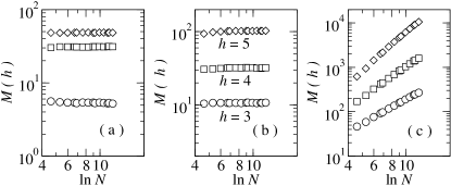
Figure 2: Numbers of $h$-loops in the ERP model with a disassortative (a), neutral (b), and assortative (c) degree-degree correlation.

Summary: We have studied the number of loops in complex networks. Discussing the scaling behaviors of percolation critical phenomena, we have shown that the structural correlation is a relevant feature of networks. The scaling behavior in the number $M_{N}(h)$ of $h$-loops for finite $h$ with network size $N$ is suggested as a signature of the correlation. When the degree distribution is not too broad, we have found that $M_{N}(h)$ is finite and independent of $N$ in one class of networks and that $M_{N}(h)$ displays the logarithmic scaling $M_{N}(h)\sim(\ln N)^{\psi_{h}}$ in the other class of networks. The former includes the uncorrelated and the RC networks. The percolation transitions in those networks are characterized with the divergent mean cluster size. The latter includes the GN models and the assortative ERG model. The display the percolation transitions with non-divergent mean cluster size. They have the assortative DD correlation commonly, although the assortativity by itself is not a sufficient condition. Our work shows that the structural correlation, reflected on the loop statistics, is important for the percolation critical phenomena. Relevance to dynamical and equilibrium critical phenomena will be studied later.

Acknowledgement: This work was supported by Korea Research Foundation Grant funded by the Korean Government (MOEHRD, Basic Research Promotion Fund) (KRF-2006-003-C00122). The author thanks Doochul Kim, Hyunggyu Park, Byungnam Kahng, and Sergey Dorogovtsev for helpful discussions.

References

- (1) D.J. Watts and S.H. Strogatz, Nature (London) 393, 440 (1998).
- (2) R. Albert and A.-L. Barabási, Rev. Mod. Phys. 74, 47 (2002).
- (3) S. Baccaletti, V. Latora, Y. Moreno, M. Chavez, and D.-U. Hwang, Phys. Rep. 424, 175 (2006).
- (4) S.N. Dorogovtsev, A.V. Goltsev, and J.F.F. Mendes, arXiv:0705.0010
- (5) D.S. Callaway, M.E.J. Newman, S.H. Strogatz, and D.J. Watts, Phys. Rev. Lett. 85, 5468 (2000).
- (6) R. Cohen, D. ben-Avraham, and S. Havlin, Phys. Rev. E 66, 036113 (2002).
- (7) D.-S. Lee, K.-I. Goh, B. Kahng, and D. Kim, Nucl. Phys. B 696, 351 (2004).
- (8) M.E.J. Newman, Phys. Rev. Lett. 89, 208701 (2002); Phys. Rev. E 67, 026126 (2003).
- (9) A. Vázquez and Y. Moreno, Phys. Rev. E 67 015101(R) (2003).
- (10) D.S. Callaway, J.E. Hopcroft, J.M. Kleinberg, M.E.J. Newman, and S.H. Strogatz, Phys. Rev. E 64, 041902 (2001).
- (11) S.N. Dorogovtsev, J.F.F. Mendes, and A.N. Samukhin, Phys. Rev. E 64, 066110 (2001).
- (12) J. Kim, P.L. Krapivsky, B. Kahng, and S. Redner, Phys. Rev. E 66, 055101(R) (2002).
- (13) P.L. Krapivsky and B. Derrida, Physica A 340,714 (2004).
- (14) J.D. Noh, arXiv:0705.0087
- (15) M. Molloy and B. Reed, Random Struct. Algorithms 6, 161 (1995).
- (16) K.-I. Goh, B. Kahng, and D. Kim, Phys. Rev. Lett. 87, 278701 (2001).
- (17) J.-S. Lee, K.-I. Goh, B. Kahng, and D. Kim, Eur. Phys. J. B 49, 231 (2006).
- (18) R. Pastor-Satorras, A. Vázquez, and A. Vespignani, Phys. Rev. Lett. 87, 258701 (2001).
- (19) S.N. Dorogovtsev, Phys. Rev. E 69, 027104 (2004).
- (20) J.D. Noh, unpublished.
- (21) J. Park and M.E.J. Newman, Phys. Rev. E 70, 066117 (2004).
- (22) J.D. Noh, G.M. Shim, and H. Lee, Phys. Rev. Lett. 94, 198701 (2005); J.D. Noh, Phys. Rev. E 72, 056123 (2005).
- (23) J.D. Noh and S.-W. Kim, J. Korean Phys. Soc. 48, S202 (2006).
- (24) G. Bianconi and A. Capocci, Phys. Rev. Lett. 90, 078701 (2003).
- (25) H.D. Rosenfeld, J.E. Kirk, E.M. Bolt, and D. ben-Avraham, J. Phys. A 38, 4589 (2005).
- (26) E. Marinari and R. Monasson, J. Stat. Mech.: Theory Exp. P09004 (2004).
- (27) G. Bianconi and M. Marsili, J. Stat. Mech.: Theory Exp. P06005 (2005).
- (28) G. Bianconi and M. Marsili, Phys. Rev. E 73, 066127 (2006).
- (29) D. Kim, in private communication.
- (30) To a given value of , one can separate the edges into three nonempty sets; one for edges among , another for edges among , and the other for edges interconnecting them. An edge in the first set adds unity to and , while one in the second set does not contribute to them. One the other hand, a edge in the third set adds unity to but nothing to . Hence one finds that for all . Since , it proves that . The equality holds only when .
- (31) A closed form expression for is not known. An exact enumeration study suggests that it grows exponentially as with .