Diffusive transport in graphene: the role of interband correlation

Abstract

We present a kinetic equation approach to investigate dc transport properties of graphene in the diffusive regime considering long-range electron-impurity scattering. In our study, the effects of interband correlation (or polarization) on conductivity are taken into account. We find that the conductivity contains not only the usual term inversely proportional to impurity density $N_{i}$, but also an anomalous term that is linear in $N_{i}$. This leads to a minimum in the density dependence of conductivity when the electron density $N_{\rm e}$ is equal to a critical value, $N_{c}$. For $N_{\rm e}>N_{c}$ the conductivity varies almost linearly with the electron density, while it is approximately inversely proportional to $N_{\rm e}$ when $N_{\rm e}<N_{c}$ in the diffusive regime. The effects of various scattering potentials on the conductivity minimum are also analyzed. Using typical experimental parameters, we find that for RPA screened electron-impurity scattering the minimum conductivity is about $5.1\,e^{2}/h$ when $N_{\rm e}\approx 0.32N_{i}$.

I Introduction

Recently, graphene has attracted a great deal of experimental and theoretical interest.NV ; NV1 ; Zhang ; Zhang1 ; Review ; Review1 In this two dimensional system, low energy electrons behave as massless relativistic fermions due to their linear energy spectrum around two nodal points in the Brillouin zone.ES Such unusual electronic properties lead to high mobility as well as a long mean free path at room temperature, making graphene a promising candidate for future electronic applications.Berger

In the first experiments involving graphene, it was found that there exists a finite ”residual” conductivity, $\sigma_{\rm res}$, in the carrier-density dependence of conductivity at zero gate voltage, and its value is about $4e^{2}/h$. Furthermore, it was found that the conductivity varies linearly with carrier density when it is large. Much theoretical effort has been devoted to quantitatively explain the observed ”residual” longitudinal conductivity. Actually, the existence of such a ”residual” conductivity in perfect (scattering-free) single-layer graphene was predicted long before its experimental confirmation.Fradkin ; Lee ; Gorbar ; Ludwig Ludwig et al. obtained different minimum values, $\sigma_{\rm res}$, using two different approaches: $\sigma_{\rm res}=(\pi/2)e^{2}/h$ using the Kubo formula and $\sigma_{\rm res}=(4/\pi)e^{2}/h$ using a definition of conductivity in the sigma model.Ludwig In many recent works, the issue has been further confused with findings of even more values of residual conductivity. In Refs. Gusynin, ; Peres, ; Katsnelson, ; Tworzydlo, $\sigma_{\rm res}=(4/\pi)e^{2}/h$ was obtained, while Ziegler predicted $\sigma_{\rm res}=\pi e^{2}/h$.Ziegler $\sigma_{\rm res}=(\pi/2)e^{2}/h$ was also obtained in Ref. Falkovsky, . More recently, Ziegler demonstrated that all these values of $\sigma_{\rm res}$ can be obtained within the Kubo formulism by taking different orders of the zero-frequency dc and zero dissipation limits.Ziegler1 Performing numerical calculations with the Kubo formula, Nomura and MacDonald obtained $\sigma_{\rm res}=(4/\pi)e^{2}/h$ in the case of short-range scattering and $\sigma_{\rm res}=4e^{2}/h$ for the Coulomb scattering case.MacDonald

Employing the Boltzmann equation, Adam, et al. demonstrated that the minimum ”residual” conductivity arises from nonvanishing electron density at zero gate voltage which may be induced by impurity potentials.DasSarma Analyzing random fluctuations of gate voltage, they found that the value of $\sigma_{\rm res}$ is not universal but depends on the impurity concentration. Apart from this particular issue, the observed almost-linear variation of conductivity with electron density can be easily understood within the Kubo formula frameworkMacDonald as well as with the Boltzmann equation.DasSarma

In this paper, we present a kinetic equation approach to investigate transport in graphene considering long-range electron(or hole)-impurity scatterings. Here, interband correlations (polarization effects) are taken into account, whereas in all previous studies, such interband correlations associated with electron/hole-impurity scatterings were ignored. We find that the conductivity in graphene contains two terms: one of which is inversely proportional to impurity density, while the other one varies linearly with the impurity density. This results in a minimum (rather than ”residual”) conductivity at a nonvanishing critical electron density, $N_{c}$, in the electron-density dependence of conductivity. For electron density $N_{\rm e}$ larger than $N_{c}$, the conductivity increases almost linearly with increasing $N_{\rm e}$, while, the conductivity is approximately inversely proportional to $N_{\rm e}$ for $N_{\rm e}<N_{c}$. We also demonstrate the effects of various scattering potentials on the conductivity minimum. Considering RPA screened electron-impurity scattering, we find that, for typical experimental parameters, the critical electron density is about $0.32N_{i}$ ($N_{i}$ is the impurity density) and the value of minimum conductivity is equal to $5.1\,e^{2}/h$.

The paper is organized as follows. In Sec. II the kinetic equation for nonequilibrium distribution functions as well as its solution are presented. Also, the conductivity is exhibited in terms of microscopically derived relaxation times. In Sec. III we present our analytical results for the conductivity for several different scattering potentials. Finally, the conclusions are summarized in Sec. IV.

II Kinetic equation and solution

II.1 Kinetic equation

In the Brillouin zone of graphene, there are six points at which the energy of carriers vanishes and the conductance band touches the valence band: ${\bf p}=(\pm 4\pi/(3\sqrt{3}a),0)$, ${\bf p}=(2\pi/(3\sqrt{3}a),\pm 2\pi/(3a))$, and ${\bf p}=(-2\pi/(3\sqrt{3}a),\pm 2\pi/(3a))$ with $a$ as the lattice spacing. These points correspond to two inequivalent Dirac nodes, $K$ and $K^{\prime}$. In present paper, we are interested in the transport of carriers in graphene with momenta near these Dirac points. The Hamiltonian of an electron with two-dimensional momentum, ${\bf p}\equiv(p_{x},p_{y})=(p\cos\phi_{\bf p},p\sin\phi_{\bf p})$, near the $v=K$ or $K^{\prime}$ Dirac nodes can be written as

$$\check{h}^{(v)}_{0}({\bf p})=\gamma[\hat{\sigma}_{x}p_{x}+{\rm sgn}(v)\hat{\sigma}_{y}p_{y}],$$ (1)

with ${\rm sgn}(v)=1$ or $-1$ for $v=K$ or $K^{\prime}$, and $\gamma\equiv\sqrt{3}\alpha a/2$ is a material constant ($\alpha$ is the hopping parameter in tight-binding approximation). $\gamma$ is equal to the Fermi velocity, which is independent of carrier density in graphene.

The Hamiltonian (1) can be diagonalized, resulting in two eigen wavefunctions, $\varphi_{\mu{\bf p}}^{(v)}({\bf r})\equiv u_{\mu}({\bf p}){\rm e}^{i{\bf p}\cdot{\bf r}}$, and two eigenvalues, $\varepsilon_{\mu}=(-1)^{\mu+1}e_{\bf p}$, with $\mu=1,2$ as the helicity index, $e_{\bf p}\equiv\gamma p$, and

$$u_{\mu}^{(v)}({\bf p})=\frac{1}{\sqrt{2}}\left(\begin{array}[]{c}{\rm e}^{(-1)^{\mu}i{\rm sgn}(v)\phi_{\bf p}}\\ 1\end{array}\right).$$ (2)

$\varepsilon_{1}({\bf p})$ and $\varepsilon_{2}({\bf p})$ are just the dispersion relations of the conduction and valence bands, respectively.

It is useful to introduce a unitary transformation, $U_{\bf p}=(u_{1}({\bf p}),u_{2}({\bf p}))$, which corresponds to a change from a pseudospin basis to a pseudo-helicity basis. Applying this transformation, the Hamiltonian (1) is diagonalized as $\hat{h}^{(v)}_{0}({\bf p})\equiv[U^{(v)}_{\bf p}]^{+}{\check{h}^{(v)}}_{0}({\bf p})U^{(v)}_{\bf p}={\rm diag}[\varepsilon_{1}({\bf p}),\varepsilon_{2}({\bf p})]$. Note that $\hat{h}^{(v)}_{0}({\bf p})$ is independent of node index $v$, indicating the existence of a valley degeneracy.

In a realistic graphene system, the carriers experience scattering by impurities. We assume that, in the pseudospin basis, the interaction between carriers and impurities can be characterized by an isotropic potential, $V(|{\bf p}-{\bf k}|)$, which corresponds to scattering a carrier from state ${\bf p}$ to state ${\bf k}$. In the pseudo-helicity basis, the scattering potential takes the transformed form, $\hat{T}_{v}({\bf p},{\bf k})=[U^{(v)}_{\bf p}]^{+}V(|{\bf p}-{\bf k}|)U^{(v)}_{\bf k}$.

We are interested in the current in a graphene system driven by a dc electric field, ${\bf E}$. In the pseudo-spin basis, this electric field can be described by a scalar potential, $V=e{\bf E}\cdot{\bf r}$, with ${\bf r}$ as the carrier coordinate. From Eq. (1) it follows that the pseudo-spin single-particle current operator, $\check{\bf j}^{(v)}({\bf p})$, has vanishing diagonal elements:

$$\check{\bf j}^{(v)}({\bf p})={\bm{\nabla}}_{\bf p}\check{h}^{(v)}_{0}({\bf p}).$$ (3)

The observed net current, given by ${\bf J}=eg_{s}\sum_{v,\bf p}{\rm Tr}[\check{\bf j}^{(v)}({\bf p})\check{\rho}^{(v)}({\bf p})]$ with $\check{\rho}^{(v)}({\bf p})$ as the pseudospin-basis distribution function and $g_{s}$ as the spin degeneracy of graphene, can be also determined in pseudo-helicity basis via

$${\bf J}=g_{s}e\sum_{v,\bf p}{\rm Tr}[\hat{\bf j}^{(v)}({\bf p})\hat{\rho}^{(v)}({\bf p})],$$ (4)

with $\hat{\bf j}^{(v)}({\bf p})\equiv[U^{(v)}_{\bf p}]^{+}\check{\bf j}^{(v)}({\bf p})U^{(v)}_{\bf p}$ and $\hat{\rho}^{(v)}({\bf p})\equiv[U^{(v)}_{\bf p}]^{+}\check{\rho}^{(v)}({\bf p})U^{(v)}_{\bf p}$ being the pseudo-helicity-basis single-particle current operator and distribution function, respectively. Explicitly, Eq. (4) can be rewritten as

$${\bf J}=g_{s}\gamma e\sum_{{\bf p},v}\frac{1}{p}\left\{{\bf p}\left[[\hat{\rho}^{(v)}]_{11}({\bf p})-[\hat{\rho}^{(v)}]_{22}({\bf p})\right]\right.$$

$$\left.+2{\rm sgn}(v)[{\bf p}\times{\bf n}]{\rm Im}\left[[\hat{\rho}^{(v)}]_{12}({\bf p})\right]\right\},$$ (5)

with $[\rho^{(v)}]_{\mu\nu}({\bf p})$ as the elements of the distribution function. In the derivation of Eq. (5), the Hermitian feature of the distribution function, i.e. $\hat{\rho}^{(v)}({\bf p})=[\hat{\rho}^{(v)}]^{+}({\bf p})$, has been used. From Eq. (5) it is evident that contributions to current arise not only from the diagonal elements of the distribution function, but also involve its off-diagonal elements.

To carry out the calculation of current in graphene, it is necessary to determine the carrier distribution function. In the pseudo-spin basis, the kinetic equation for the distribution, $\check{\rho}^{(v)}({\bf p})$, can be written as

$$e{\bf E}\cdot\nabla_{\bf p}\check{\rho}^{(v)}({\bf p})+i[\check{h}^{(v)}_{0}({\bf p}),\check{\rho}^{(v)}({\bf p})]=-\check{I}^{(v)},$$ (6)

with $\check{I}^{(v)}$ as the collision term. Applying the unitary transformation $U^{(v)}_{\bf p}$, the kinetic equation for the distribution in the pseudo-helicity basis, $\hat{\rho}^{(v)}({\bf p})$, takes the form

$$e{\bf E}\cdot\left\{\nabla_{\bf p}\hat{\rho}^{(v)}({\bf p})+\left[\hat{\rho}({\bf p}),\nabla_{\bf p}\left(U^{(v)}_{\bf p}\right)^{+}U^{(v)}_{\bf p}\right]\right\}$$

$$+i[\hat{h}^{(v)}_{0}({\bf p}),\hat{\rho}^{(v)}({\bf p})]=-\hat{I}^{(v)},$$ (7)

with $\hat{I}^{(v)}=[U^{(v)}_{\bf p}]^{+}\check{I}^{(v)}[U^{(v)}_{\bf p}]$.

It should be noted that the second term on the left-hand side of Eq. (7) is associated with interband tunneling since the off-diagonal elements of matrix $e{\bf E}\cdot{\bm{\nabla}}_{\bf p}\left(U^{(v)}_{\bf p}\right)^{+}U^{(v)}_{\bf p}$ are just the interband-tunneling matrix elements $<u_{\mu}^{(v)}({\bf p})|e{\bf E}\cdot{\bf r}|u_{\bar{\mu}}^{(v)}({\bf p})>$ ($\bar{\mu}=3-\mu$) with ${\bf r}$ as carrier coordinate.Inter2 ; Interband This term of Eq. (7) results in a component of $[\hat{\rho}^{(v)}]_{12}({\bf p})$ which depends on the strength of electric field via ${\rm e}^{-b/E}$ ($b$ is a real, positive parameter), and is much less than unity in the linear response regime. Thus, the interband tunneling term of Eq. (7) is not actually linear (despite its formal appearance), and, in fact, it can be ignored at low fields. Hence, Eq. (7) can be rewritten as

$$e{\bf E}\cdot\nabla_{\bf p}\hat{\rho}^{(v)}({\bf p})+i[\hat{h}^{(v)}_{0}({\bf p}),\hat{\rho}^{(v)}({\bf p})]=-\hat{I}^{(v)},$$ (8)

with $\hat{I}^{(v)}$ as the collision term given by

$$\hat{I}^{(v)}={\hat{\Sigma}}^{r}_{v\bf p}{\hat{\rm G}}^{<}_{v\bf p}+{\hat{\Sigma}}^{<}_{v\bf p}{\hat{\rm G}}^{a}_{v\bf p}-{\hat{\rm G}}^{r}_{v\bf p}{\hat{\Sigma}}^{<}_{v\bf p}-{\hat{\rm G}}^{<}_{v\bf p}{\hat{\Sigma}}^{a}_{v\bf p}.$$ (9)

Here, ${\hat{\rm G}}^{r,a,<}_{v\bf p}$ and ${\hat{\Sigma}}^{r,a,<}_{v\bf p}$, respectively, are the nonequilibrium Green’s functions and self-energies for carriers near node $v=K$ or $K^{\prime}$.

In the kinetic equation above, electron-impurity scattering is embedded in the self-energies, ${\check{\Sigma}}^{r,a,<}_{v\bf p}$. In the present paper, we only consider electron-impurity collisions in the self-consistent Born approximation. It is widely accepted that this is sufficiently accurate to analyze transport properties in the diffusive regime.Jauho Accordingly, the self-energies take the forms:

$$\hat{\Sigma}^{r,a,<}_{v\bf p}=n_{i}\sum_{{\bf k}}\hat{T}_{v}({\bf p},{\bf k})\hat{\rm G}^{r,a,<}_{v\bf k}\hat{T}_{v}^{+}({\bf p},{\bf k}).$$ (10)

In the present paper, we restrict our considerations to the linear response regime. In connection with this, all the functions, such as the nonequilibrium Green’s functions, self-energies, and distribution function, can be expressed as sums of two terms: $A=A_{0}+A_{1}$, with $A$ representing the Green’s functions, self-energies or distribution function. $A_{0}$ and $A_{1}$, respectively, are the unperturbed part and the linear electric field part of $A$. In these terms, the kinetic equation for the linear electric field part of the distribution, $\hat{\rho}^{(v)}_{1}({\bf p})$, takes the form

$$e{\bf E}\cdot\nabla_{\bf p}\hat{\rho}^{(v)}_{0}({\bf p})+i\left[\hat{h}^{(v)}_{0},\hat{\rho}^{(v)}_{1}({\bf p})\right]=-\hat{I}_{v}^{(1)},$$ (11)

with $\hat{I}_{v}^{(1)}$ as the linear electric field part of the collision term $\hat{I}_{v}$. This equation can be further rewritten explicitly as

$$e{\bf E}\cdot\nabla_{\bf p}[\hat{\rho}^{(v)}_{0}]_{\mu\mu}({\bf p})=-[\hat{I}^{(1)}_{s}]_{\mu\mu},$$ (12)

and

$$2i\gamma p[\hat{\rho}^{(v)}_{1}]_{12}({\bf p})=-[\hat{I}^{(1)}_{s}]_{12},$$ (13)

with $(\hat{\rho}_{1})_{\mu\nu}({\bf p})$ and $(\hat{\rho}_{0})_{\mu\mu}({\bf p})$, respectively, as the elements of $\hat{\rho}_{1}({\bf p})$ and $\hat{\rho}^{(v)}_{0}({\bf p})={\rm diag}[n_{\rm F}(\varepsilon_{1}({\bf p})),n_{\rm F}(\varepsilon_{1}({\bf p}))]$, and ${\bf n}$ is a unit vector perpendicular to the graphene plane.

To further simplify Eq. (11), we employ a two-band generalized Kadanoff-Baym ansatz (GKBA).GKBA ; GKBA1 This ansatz, which expresses the lesser Green’s function in terms of the Wigner distribution function, has been proven sufficiently accurate to analyze transport and optical properties in semiconductors.Jauho To first order in the dc field strength, the GKBA reads,

$$\hat{\rm G}^{<}_{1}({\bf p},\omega)=-\hat{\rm G}_{0}^{r}({\bf p},\omega)\hat{\rho}_{1}({\bf p})+\hat{\rho}_{1}({\bf p})\hat{\rm G}_{0}^{a}({\bf p},\omega),$$ (14)

where the unperturbed retarded and advanced Green’s functions are diagonal: $\hat{\rm G}_{0}^{r,a}({\bf p},\omega)={\rm diag}[(\omega-\varepsilon_{1}({\bf p})\pm i\delta)^{-1},(\omega-\varepsilon_{2}({\bf p})\pm i\delta)^{-1}]$. In our treatment, the effect of $\hat{\rm G}_{1}^{r,a}({\bf p},\omega)$ on the distribution function has been ignored because these linear electric field parts of the retarded and advanced Green’s functions lead to a collisional broadening effect on $\hat{\rho}_{1}({\bf p})$, which plays a secondary role in transport studies. Further, in our treatment, we ignore intervalley transitions of carriers between different Dirac points since the corresponding rates are very small in the presence of carrier-impurity scattering.

Within the framework of these considerations, the scattering term $\hat{I}^{(1)}_{v}$ in Eq. (11) can be expressed in terms of the distribution function: its diagonal elements, $[\hat{I}^{(1)}_{v}]_{\mu\mu}$, can be written as

$$[\hat{I}^{(1)}_{v}]_{\mu\mu}=\pi N_{i}\sum_{{\bf k}}|V({\bf p}-{\bf k})|^{2}\delta[\varepsilon^{(v)}_{\mu}({\bf p})-\varepsilon^{(v)}_{\mu}({\bf k})]$$

$$\times\left\{[1+\cos(\phi_{\bf p}-\phi_{\bf k})]\{[\hat{\rho}_{1}^{(v)}]_{\mu\mu}({\bf p})-[\hat{\rho}_{1}^{(v)}]_{\mu\mu}({\bf k})\}\right.$$

$$-(-1)^{\mu}{\rm sgn}(v)\sin(\phi_{\bf p}-\phi_{\bf k})\left.{\rm Im}\{[\hat{\rho}_{1}^{(v)}]_{12}({\bf p})+[\hat{\rho}_{1}^{(v)}]_{12}({\bf k})\}\right\}$$ (15)

while the off-diagonal element, $[\hat{I}^{(1)}_{v}]_{12}$, takes the form

$$[\hat{I}^{(1)}_{v}]_{12}=\frac{\pi N_{i}}{2}\sum_{{\bf k},\mu}|V({\bf p}-{\bf k})|^{2}\delta[\varepsilon^{(v)}_{\mu}({\bf p})-\varepsilon^{(v)}_{\mu}({\bf k})]$$

$$\times\left\{(-1)^{\mu+1}i{\rm sgn}(v)\sin(\phi_{\bf p}-\phi_{\bf k})\{[\hat{\rho}_{1}^{(v)}]_{\mu\mu}({\bf p})-[\hat{\rho}_{1}^{(v)}]_{\mu\mu}({\bf k})\}\right.$$

$$+[1-\cos(\phi_{\bf p}-\phi_{\bf k})]\left.\{[\hat{\rho}_{1}^{(v)}]_{12}({\bf p})-[\hat{\rho}_{1}^{(v)}]_{21}({\bf k})\}\right\}.$$ (16)

In the derivation of these equations, the effects of the real parts of the retarded and advanced Green’s functions on $\hat{I}^{(1)}_{v}$ have been ignored.

II.2 Conductivity and solution of the kinetic equation

Since $\varepsilon_{\mu}({\bf p})$, as well as the equilibrium distribution $\hat{\rho}^{(v)}_{0}({\bf p})$, depend only on the magnitude of momentum, the dependence of $\hat{\rho}^{(v)}_{1}({\bf p})$ on momentum angle can be evaluated explicitly. From Eq. (11) we see that the diagonal elements of $\hat{\rho}^{(v)}_{1}({\bf p})$ can be written as [${\bf v}^{(v)}_{\mu}({\bf p})={\bm{\nabla}}_{\bf p}\varepsilon_{\mu}^{(v)}({\bf p})=(-1)^{\mu+1}\gamma{\bf p}/p$]

$$[\hat{\rho}_{1}^{(v)}]_{\mu\mu}({\bf p})=e{\bf E}\cdot{\bf v}^{(v)}_{\mu}({\bf p})\Lambda^{(v)}_{\mu}(p),$$ (17)

while the off-diagonal element, $[\hat{\rho}_{1}^{(v)}]_{12}({\bf p})$ , takes the form

$$[\hat{\rho}_{1}^{(v)}]_{12}({\bf p})=\frac{e\gamma}{p}[{\bf E}\times{\bf p}\cdot{\bf n}]\Phi^{(v)}(p).$$ (18)

The functions $\Lambda^{(v)}_{\mu}(p)$ and $\Phi^{(v)}(p)$ depend only on the magnitude of momentum and are determined by coupled equations:

$$-\frac{\partial\{[\hat{\rho}^{(v)}_{0}]_{\mu\mu}({\bf p})\}}{\partial\varepsilon^{(v)}_{\mu}({\bf p})}=\frac{1}{\tau_{\mu}^{(a)}(p)}\left\{\Lambda_{\mu}^{(v)}(p)-{\rm sgn}(v){\rm Im}[\Phi^{(v)}(p)]\right\},$$ (19)

$$2\gamma p{\rm Re}[\Phi^{(v)}(p)]=\sum_{\mu}\frac{1}{2\tau^{(a)}_{\mu}(p)}$$

$$\times\left\{{\rm sgn}(v)\Lambda_{\mu}^{(v)}(p)-{\rm Im}[\Phi^{(v)}(p)]\right\},$$ (20)

and

$$2\gamma p{\rm Im}[\Phi^{(v)}(p)]=\sum_{\mu}\frac{1}{2\tau^{(b)}_{\mu}(p)}\left\{{\rm Re}[\Phi^{(v)}(p)]\right\},$$ (21)

with $\tau^{(a,b)}_{\mu}(p)$ as microscopically determined relaxation times independent of node index $v$: $[\tau^{(a,b)}_{\mu}(p)]^{-1}=\pi N_{i}\sum_{\bf k}|V({\bf p}-{\bf k})|^{2}\delta[\varepsilon_{\mu}({\bf p})-\varepsilon_{\mu}({\bf k})]A^{(a,b)}(\phi_{\bf k})$; $A^{(a)}(\phi)=\sin^{2}\phi$, and $A^{(b)}(\phi)=(1-\cos\phi)^{2}$. Solving the algebraic equations (19)-(21) yields explicit analytic expressions for the functions $\Lambda_{\mu}^{(v)}$ and $\Phi^{(v)}(p)$ in terms of the relaxation times as

$${\rm Re}[\Phi^{(v)}(p)] = -\frac{{\rm sgn}(v)}{4\gamma^{2}p^{2}}\sum_{\mu}\left\{\gamma p\frac{\partial\{[\hat{\rho}_{0}^{(v)}]_{\mu\mu}({\bf p})\}}{\partial\varepsilon^{(v)}_{\mu}({\bf p})}\right\},$$ (22)

$${\rm Im}[\Phi^{(v)}(p)]=-\frac{{\rm sgn}(v)}{16\gamma^{3}p^{3}}\left[\frac{1}{\tau^{(b)}_{1}(p)}+\frac{1}{\tau^{(b)}_{2}(p)}\right]$$

$$\times\sum_{\mu}\left[\gamma p\frac{\partial\{[\hat{\rho}_{0}^{(v)}]_{\mu\mu}({\bf p})\}}{\partial\varepsilon^{(v)}_{\mu}({\bf p})}\right],$$ (23)

and

$$\Lambda^{(v)}_{\mu}(p)=-\tau^{(a)}_{\mu}(p)\frac{\partial\{[\hat{\rho}_{0}^{(v)}]_{\mu\mu}({\bf p})]}{\partial\varepsilon^{(v)}_{\mu}({\bf p})}$$

$$+{\rm sgn}(v){\rm Im}[\Phi^{(v)}(p)].$$ (24)

Substituting Eqs. (17) and (18) into Eq. (5), ${\bf J}$ can be further rewritten as

$${\bf J}=\frac{e^{2}}{2}g_{s}\gamma^{2}{\bf E}\sum_{{\bf p},v}\{[\Lambda^{(v)}_{1}(p)+\Lambda^{(v)}_{2}({p})]\\ +2{\rm sgn}(v){\rm Im}[\Phi^{(v)}({p})]\}.$$

Inserting the explicit forms of $\Lambda^{(v)}_{\mu}(p)$ and $\Phi^{(v)}({p})$, we find that the conductivity, $\sigma$, takes the form

$$\sigma=-\frac{e^{2}}{2}g_{s}\gamma^{2}\sum_{{\bf p},\mu,v}\left\{\left[\tau^{(a)}_{\mu}(p)+\frac{1}{4\gamma^{2}p^{2}\tau^{(b)}(p)}\right]\right.$$

$$\times\left.\frac{\partial\left\{[\hat{\rho}_{0}^{(v)}]_{\mu\mu}({\bf p})\right\}}{\partial\varepsilon^{(v)}_{\mu}({\bf p})}\right\},\,\,\,\,\,\,\,$$ (25)

with $[\tau^{(b)}(p)]^{-1}\equiv[\tau^{(b)}_{1}(p)]^{-1}+[\tau^{(b)}_{2}(p)]^{-1}$.

From Eq. (25) it is clear that, the conductivity in graphene involves not only a term proportional $N_{i}^{-1}$, but also a term linear in impurity density. However, there is no term independent of impurity scattering. This differs significantly from previous results. Adams et al. and Galitski et al. found the conductivity to always be proportional to $N_{i}^{-1}$,DasSarma ; DasSarma2 while the other previous calculations indicated that the conductivity always contains a term independent of impurity scattering.Ludwig ; Gusynin ; Peres ; Katsnelson ; Tworzydlo ; Ziegler ; Falkovsky ; Ziegler1 ; MacDonald

It should be noted that the anomalous conductivity term proportional to $N_{i}$ arises from the nonvanishing of $[\hat{\rho}_{1}^{(v)}]_{12}({\bf p})$. This can be seen from Eq. (II.2): the conductivity depends on the imaginary part of $[\hat{\rho}_{1}^{(v)}]_{12}({\bf p})$, which is proportional to $[{\tau^{(b)}_{\mu}(p)}]^{-1}$. Since $[\hat{\rho}_{1}^{(v)}]_{12}({\bf p})$ describes interband coherence, the anomalous conductivity term is a result of interband correlation.

From Eqs. (20) and (21) it follows that the imaginary part of $[\hat{\rho}_{1}^{(v)}]_{12}({\bf p})$ is proportional to $N_{i}$, while its real part is independent of impurity density. This can be understood from the fact that both the driving electric field and impurity scattering can cause transitions between two pseudo-helicity states: they result in a change of carrier momentum but retain the pseudospin unchanged, leading to a change of pseudo-helicity. Obviously, the probability of this transition is proportional to the strength of the momentum change, which is determined by the electric field and/or by impurity scattering. Thus, impurity scattering results in a term of $[\hat{\rho}_{1}^{(v)}]_{12}({\bf p})$ proportional to $N_{i}$, while the $N_{i}$-independent term of $[\hat{\rho}_{1}^{(v)}]_{12}({\bf p})$ is a result of the momentum change induced directly by the electric field.

III Results and discussion

As pointed out by Adam, et al., ”intrinsic graphene” with chemical potential (or Fermi energy) precisely at the Dirac point is experimentally unrealizable since charged impurity disorder or spatial inhomogeneity in the system can lead to a nonvanishing induced graphene carrier density.DasSarma Accordingly, all experimental graphene samples are extrinsic since some free carriers always exist in the system. In connection with this, the conductivity of graphene arises mainly from the contribution of one type of carrier, electrons or holes, depending on the experimental conditions.

In the present paper, we focus on electron transport in graphene at zero temperature. In this case, the chemical potential (or, equivalently the Fermi energy, $E_{F}$) is given by $E_{F}=\gamma k_{F}$ with the 2D Fermi wavevector $k_{F}$ depending on the electron density through $k_{F}=\sqrt{4\pi N_{\rm e}/g_{s}g_{v}}$ ( we choose the spin and valley degeneracies, respectively, as $g_{s}=g_{v}=2$ in the present paper). The zero-temperature conductivity is given by

$$\left.\sigma\right|_{T=0}={e^{2}}\frac{g_{s}g_{v}}{4\pi}\gamma k_{F}\left[\tau^{(a)}_{1}(k_{F})+\frac{1}{4\gamma^{2}k_{F}^{2}\tau^{(b)}(k_{F})}\right].$$ (26)

To analyze the effects of scattering potentials on $\sigma$, we consider short-range (SR), Thomas-Fermi (TF), as well as random-phase-approximation (RPA) screened Coulomb interactions.

Short-range screened Coulomb interaction- For a short-range screened interaction potential, $V({\bf p}-{\bf k})$ becomes independent of electron momentum: $V({\bf p}-{\bf k})\approx\pi\gamma/(2k_{F})$.MacDonald In connection with this, the relaxation times $\tau^{(a)}_{1}(k_{F})$ and $\tau^{(b)}(k_{F})$, respectively, reduce to $\tau^{(a)}_{1}(k_{F})=16N_{\rm e}/(N_{i}\pi\gamma k_{F})$ and $\tau^{(b)}(k_{F})=8N_{\rm e}/(3\pi N_{i}\gamma k_{F})$. Thus, the zero-temperature conductivity for a short-range potential, $\left.\sigma\right|^{\rm SR}_{T=0}$, reduces to

$$\left.\sigma\right|^{\rm SR}_{T=0}=\frac{e^{2}}{\pi}\left[\frac{16N_{\rm e}}{\pi N_{i}}+\frac{3\pi N_{i}}{32N_{\rm e}}\right].$$ (27)

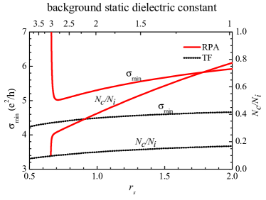
Figure 1: The dependencies of minimum conductivity and critical density on $r_{s}$ for TF and RPA screened Coulomb potentials. $\gamma$ is chosen to be $1.1\times 10^{5}$m/s.

Thomas-Fermi screened potential- We also evaluate the conductivity for a 2D Thomas-Fermi screened potential, $V^{\rm TF}(q)$, given by

$$V^{\rm TF}(q)=\frac{e^{2}}{2\pi\varepsilon_{0}\kappa(q+q_{s})},$$ (28)

with ${\bf q}\equiv{\bf p}-{\bf k}$, $q_{s}=4e^{2}k_{F}/(\kappa\gamma)$ and $\kappa$ as the static background dielectric constant. In this case, the scattering times $\tau^{(a)}_{1}(k_{F})$ and $\tau^{(b)}(k_{F})$ can be obtained analytically as:

$$\left[\frac{1}{\tau^{(a)}_{1}(k_{F})}\right]_{\rm TF}=\frac{N_{i}}{N_{\rm e}}\gamma k_{F}G(2r_{s}),$$ (29)

and

$$\left[\frac{1}{\tau^{(b)}(k_{F})}\right]_{\rm TF}=\frac{N_{i}}{N_{\rm e}}\gamma k_{F}F(2r_{s}),$$ (30)

with $r_{s}=e^{2}/(4\pi\varepsilon_{0}\kappa\gamma)$. The functions $G(x)$ and $F(x)$ are defined as

$$G(x) = \frac{x^{2}}{8}\int_{0}^{2\pi}d\theta\frac{\sin^{2}\theta}{(\sin\frac{\theta}{2}+x)^{2}}$$ (33)

$$= x^{2}\left\{\begin{array}[]{ll}\frac{\pi}{4}+3x-\frac{3\pi}{2}x^{2}+{|x|(3x^{2}-2)\arccos(1/x)}[{x^{2}-1}]^{-1/2}&|x|>1\\ \frac{\pi}{4}+3x-\frac{3\pi}{2}x^{2}+{x(3x^{2}-2){\rm Re}\left[{\rm arctanh}(1/\sqrt{1-x^{2}})\right]}[{1-x^{2}}]^{-1/2}&0\leq x\leq 1\end{array}\right.,$$

and

$$F(x) = \frac{x^{2}}{8}\int_{0}^{2\pi}d\theta\frac{(1-\cos\theta)^{2}}{(\sin\frac{\theta}{2}+x)^{2}}$$ (36)

$$= x^{2}\left\{\begin{array}[]{ll}\frac{\pi}{2}-4x+3x^{2}\pi-\frac{2x^{3}}{x^{2}-1}+{|x^{3}|(8-6x^{2})\arccos(1/x)}{(x^{2}-1)^{-3/2}}&|x|>1\\ \frac{\pi}{2}-4x+3x^{2}\pi-\frac{2x^{3}}{x^{2}-1}-{x^{3}(8-6x^{2}){\rm Re}\left[{\rm arctanh}(1/\sqrt{1-x^{2}})\right]}{(1-x^{2})^{-3/2}}&0\leq x\leq 1\end{array}\right..$$

Thus, the conductivity for the TF potential, $\left.\sigma\right|^{\rm TF}_{T=0}$, is determined by

$$\left.\sigma\right|^{\rm TF}_{T=0}=\frac{e^{2}}{\pi}\left[\frac{N_{\rm e}}{N_{i}G(2r_{s})}+\frac{N_{i}F(2r_{s})}{4N_{\rm e}}\right].$$ (37)

RPA-screened Coulomb potential- We also examine the conductivity of graphene in the presence of RPA-screened electron-impurity scattering, with the potential taking the form:

$$V(q)=\frac{e^{2}}{2\pi\varepsilon_{0}\kappa q\varepsilon(q)},$$ (38)

and the dielectric function $\varepsilon(q)$ for the massless Dirac energy spectrum is given byAndo ; DasSarma1

$$\varepsilon(q)=1+\frac{q_{s}}{q}\left\{\theta(2k_{F}-q)\left(1-\frac{\pi q}{8k_{F}}\right)\right.$$

$$\left.+\theta(q-2k_{F})\left[1-\frac{1}{2}\sqrt{1-\left(2k_{F}/q\right)^{2}}\right.\right.$$

$$\left.\left.-\frac{q}{4k_{F}}\arcsin(2k_{F}/q)\right]\right\}.$$ (39)

Substituting the RPA-screened potential into the expressions for the scattering times, we obtain

$$\left[\frac{1}{\tau^{(a)}_{1}(k_{F})}\right]_{\rm RPA}=\frac{N_{i}}{N_{\rm e}}\gamma k_{F}G[4r_{s}/(2-\pi r_{s})],$$ (40)

and

$$\left[\frac{1}{\tau^{(b)}(k_{F})}\right]_{\rm RPA}=\frac{N_{i}}{N_{\rm e}}\gamma k_{F}F[4r_{s}/(2-\pi r_{s})].$$ (41)

Hence, from Eq. (26), it follows that the conductivity for the RPA-screened Coulomb potential case is given by

$$\left.\sigma\right|^{\rm RPA}_{T=0}=\frac{e^{2}}{\pi}\left[\frac{N_{\rm e}}{N_{i}G[4r_{s}/(2-\pi r_{s})]}\right.$$

$$\left.+\frac{N_{i}F[4r_{s}/(2-\pi r_{s})]}{4N_{\rm e}}\right].$$ (42)

From Eqs.(27), (37), and(42) it is evident that a minimum exists in the electron-density dependence of graphene conductivity for short-range, Thomas-Fermi as well as RPA-screened Coulomb potentials. The corresponding critical values of electron density, $N_{c}$, and the minimum conductivities, $\sigma_{\rm min}$, are shown in table I. Furthermore, we verify that, for $N_{\rm e}>N_{c}$, the conductivity varies almost linearly with the electron density, while it is inversely proportional to $N_{\rm e}$ when $N_{\rm e}<N_{c}$.

	$N_{c}/N_{i}$	$\sigma_{\rm min}/(e^{2}/h)$
SR	$\pi\sqrt{6}/32\approx 0.24$	$2\sqrt{6}\approx 4.9$
TF	$\sqrt{F(2r_{s})G(2r_{s})}/2$	$2[\sqrt{F(2r_{s})/G(2r_{s})}]$
RPA	$\sqrt{F[4r_{s}/(2-\pi r_{s})]G[4r_{s}/(2-\pi r_{s})]}/2$	$2\{\sqrt{F[4r_{s}/(2-\pi r_{s})]/G[4r_{s}/(2-\pi r_{s})]}\}$

Table 1: Critical electron densities and minimum conductivities for the various screened Coulomb potentials considered

From Eq. (27) we see that, for SR screened scattering, $N_{c}/N_{i}$ and $\sigma_{\rm min}$ are constants independent of $r_{s}$. However, for the TF and RPA potentials, they are functions of $r_{s}$, which is, in principle, a tunable parameter through its dependence on the background dielectric constant $\kappa$. In Fig. 1, we plot the dependencies of $N_{c}$ and $\sigma_{\rm min}$ on $r_{s}$. This figure enables us to determine the values of $\sigma_{\rm min}$ and $N_{c}$ for various experimental samples.

Experimentally, graphene is usually fabricated using a SiO₂ substrate and hence the background static dielectric constant,, $\kappa$, can be estimated as $\kappa=2.45$.DasSarma The measured Fermi velocity $\gamma=1.1\times 10^{5}$m/s leads to $r_{s}\approx 0.813$.Zhang For this $r_{s}$ value, we obtain

$$\sigma_{\rm min}^{\rm TF}\approx 4.42e^{2}/h, N_{c}^{\rm TF}\approx 0.11N_{i},$$ (43)

$$\sigma^{\rm RPA}_{\rm min}\approx 5.11e^{2}/h, N_{c}^{\rm RPA}\approx 0.32N_{i}.$$ (44)

Furthermore, the asymptotic dependence of conductivity on electron density as $N_{\rm e}$ moves away from the critical value is given in the TF and RPA cases as:

$$\left.\sigma\right|^{\rm TF}_{T=0}\longrightarrow\frac{e^{2}}{h}\left\{\begin{array}[]{cc}{20.0N_{\rm e}}/{N_{i}}&N_{\rm e}>N_{c}^{\rm TF}\\ {0.25N_{i}}/{N_{\rm e}}&N_{\rm e}<N_{c}^{\rm TF}\\ \end{array}\right.,$$ (45)

$$\left.\sigma\right|^{\rm RPA}_{T=0}\longrightarrow\frac{e^{2}}{h}\left\{\begin{array}[]{cc}{8.0N_{\rm e}}/{N_{i}}&N_{\rm e}>N_{c}^{\rm RPA}\\ {0.8N_{i}}/{N_{\rm e}}&N_{\rm e}<N_{c}^{\rm RPA}\\ \end{array}\right..$$ (46)

The experimentally observed residual conductivity is about $4e^{2}/h$ and our obtained minimum conductivity is in good quantitative agreement with it. The contention of Adam, et al., about finite electron density at zero gate voltage is plausible in describing the observed plateau near zero gate voltage.DasSarma However, the vagaries of earlier theories described in the Introduction, and our own prediction of an unlimited increase of conductivity with decreasing $N_{\rm e}$ for $N_{\rm e}<N_{c}$ (which tends to infinity as $N_{\rm e}\rightarrow 0$) calls for a re-evaluation of the assumption of linearity. We believe that the problematic theoretical density dependence of conductivity for low $N_{\rm e}$ is associated with the fact that, in the dilute limit, the response of the system caused by the electric field can not be treated as linear in $|{\bf E}|$. It is well known that linear response theory is valid only for $e|{\bf E}|\alpha<\gamma k_{F}$ with $\alpha\equiv<{\bf r}>\approx\gamma\tau$ as the average displacement induced by the electric field ($\tau$ is the relaxation time). In the dilute limit, $k_{F}$ is very small and the requirement $e|{\bf E}|\alpha<\gamma k_{F}$ is difficult to satisfy experimentally. Hence, our theory, as well as other linear response theories, can not be employed to describe the transport behavior of carriers in real systems with $N_{\rm e}\rightarrow 0$.

IV Conclusions

We have formulated a kinetic equation to investigate dc transport in graphene considering long-range electron-impurity scatterings. In this study, we included the role of interband correlations. We found that the conductivity contains two terms: one term is inversely proportional to the impurity density while the other one is linear in $N_{i}$. This results in a minimum in the density dependence of conductivity for $N_{\rm e}$ equal to a critical density, $N_{c}$. For $N_{\rm e}>N_{c}$ the conductivity varies almost linearly with the electron density while, for $N_{\rm e}<N_{c}$, $\sigma$ is approximately inversely proportional to $N_{\rm e}$. We also discussed the effects of various scattering potentials on the conductivity minimum. Using typical experimental parameters, we found that for the RPA-screened Coulomb potential, $\sigma_{\rm min}\approx 5.1\,e^{2}/h$ and $N_{c}\approx 0.32N_{i}$.

- (1) K.S. Novoselov, A.K. Geim, S.V. Morozov, D. Jiang, Y. Zhang, S.V. Dubonos, I.V. Grigorieva, and A.A. Firsov, Science 306, 666 (2004).
- (2) K.S. Novoselov, A.K. Geim, S.V. Morozov, D. Jiang, M. I. Katsnelson, I.V. Grigorieva, S.V. Dubonos, and A.A. Firsov, Nature 438, 197 (2005).
- (3) Y. Zhang, J. P. Small, M. E. S. Amori, and P. Kim, Phys. Rev. Lett. 94, 176803 (2005).
- (4) Y. Zhang, Y.-W. Tan, H. L. Stormer, and P. Kim, Nature (London) 438, 201 (2005).
- (5) M.L. Katsnelson, Materials Today 10, 20 (2006).
- (6) A. H. Castro Neto, F. Guinea, N. M. R. Peres, K. S. Novoselov, and A. K. Geim, arXiv: 0709.1163 (unpublished).
- (7) G.W. Semenoff, Phys. Rev. Lett. 53, 2449 (1984); F.D.M. Haldane, ibid 61, 2015 (1988).
- (8) C. Berger, Z. Song, X. Li, X. Wu, N. Brown, C. Naud, D. Mayou, T. Li, J. Hass, A.N. Machenkov, E.H. Conrad, P.N. First and W.A. de Heer, Science 312, 1191 (2006).
- (9) E. Fradkin, Phys. Rev. B 33, 3263 (1986).
- (10) P. A. Lee, Phys. Rev. Lett. 71, 1887 (1993).
- (11) E. V. Gorbar, V. P. Gusynin, V. A. Miransky, and I. A. Shovkovy, Phys. Rev. B 66, 045108 (2002).
- (12) A. W. W. Ludwig, M. P. A. Fisher, R. Shankar, and G. Grinstein, Phys. Rev. B 50, 7526 (1994).
- (13) V. P. Gusynin and S. G. Sharapov, Phys. Rev. Lett. 95, 146801 (2005).
- (14) N. M. R. Peres, F. Guinea, and A. H. Castro Neto, Phys. Rev. B 73, 125411 (2006).
- (15) M. I. Katsnelson, Eur. Phys. J. B 51, 157 (2006).
- (16) J. Tworzydlo, B. Trauzettel, M. Titov, A. Rycerz, and C. W. J. Beenakker, Phys. Rev. Lett. 96, 246802 (2006).
- (17) K. Ziegler, Phys. Rev. Lett. 97, 266802 (2006).
- (18) L. A. Falkovsky and A. A. Varlamov, cond-mat/0606800 (unpublished).
- (19) K. Ziegler, cond-mat/0701300 (unpublished).
- (20) K. Nomura and A. H. MacDonald, Phys. Rev. Lett. 98, 076602 (2007).
- (21) S. Adam, E. H. Hwang, V. M. Galitski, and S. Das Sarma, Proc. Natl. Acad. Sci. USA 104, 18392 (2007).
- (22) V. M. Galitski, S. Adam, and S. Das Sarma, cond-mat/0702117 (unpublished).
- (23) J.Callaway, Quantum Theory of the Solid State, 2nd ed. (Academic, Boston, 1991), p. 481.
- (24) J. B. Krieger and G. J. Iafrate, Phys. Rev. B 33, 5494 (1986); ibid. 35, 9644 (1987).
- (25) P. Lipavský, V. Špička, and B. Velicky, Phys. Rev. B 34, 6933 (1986).
- (26) H. Haug, Phys. Status Solidi (b) 173, 139 (1992).
- (27) H. Haug and A.-P. Jauho, Quantum Kinetics in Transport and Optics of Semiconductors (Springer, 1996).
- (28) T. Ando, J. Phys. Soc. Jpn. 75, 074716 (2006).
- (29) E. H. Hwang and S. Das Sarma, Phys. Rev. B 75, 205418 (2007).