Long term ordering kinetics of the two dimensional q-state Potts model

Abstract

We studied the non-equilibrium dynamics of the q-state Potts model in the square lattice, after a quench to sub-critical temperatures. By means of a continuous time Monte Carlo algorithm (non-conserved order parameter dynamics) we analyzed the long term behavior of the energy and relaxation time for a wide range of quench temperatures and system sizes. For $q>4$ we found the existence of different dynamical regimes, according to quench temperature range. At low (but finite) temperatures and very long times the Lifshitz-Allen-Cahn domain growth behavior is interrupted with finite probability when the system stuck in highly symmetric non-equilibrium metastable states, which induce activation in the domain growth, in agreement with early predictions of Lifshitz [JETP 42, 1354 (1962)]. Moreover, if the temperature is very low, the system always gets stuck at short times in a highly disordered metastable states with finite life time, which have been recently identified as glassy states. The finite size scaling properties of the different relaxation times involved, as well as their temperature dependency are analyzed in detail.

I Introduction

The problem of domain growth kinetics in systems with many degenerate ground states had attracted a lot of attention in the pastLifshitz (1962); Safran (1981); Vinals and Grant (1987); Grest et al. (1988); Kumar et al. (1987); Sire and Majumdar (1995). In early works LifshitzLifshitz (1962) and then SafranSafran (1981) posed the discussion about the effect of activated processes in the domain growth. They suggested that $d$-dimensional, $q$-state degenerate models could become trapped in local metastable states for $q\geq d+1$, which would then greatly slow down the relaxational kinetics. Their argument in two dimensions is that a honeycomb structure of hexagonal domains is stable under small distortions of the interfaces, because such distortions do not increase the interfacial free energy. Large distortions due to fluctuations are then needed to move the interfaces and so domain growth becomes activated. The prototype of such a system is the q-state Potts modelWu (1982), whose Hamiltonian is given by

$$H=-J~{}\sum_{nn}\delta(s_{i},s_{j})\qquad J>0$$ (1)

where $s_{i}=1,2,\ldots,q$, $\delta(s_{i},s_{j})$ is the Kronecker delta and the sum runs over all the pairs of nearest-neighbor sites. Viñals and GrantVinals and Grant (1987) performed Monte Carlo (MC) simulations with Glauber dynamics for $q=8$ in square lattices of size up to $N=128^{2}$ sites and time scales of the order $10^{4}$ Monte Carlo Steps (MCS) (1 MCS is defined as as a complete cycle of $N$ spin update trials, according to a Metropolis MC algorithm). They found evidences of metastable configurations composed by squares of different colors (i.e., different values of $q$) that freeze the dynamics a $T=0$. Moreover, they argue that those configurations only effectively dominate at $T=0$ and growth at finite temperatures is not limited by activated processesVinals and Grant (1987). Hence, for long enough times the average linear domain size should follow the Lifshitz-Allen-Cahn (LAC) law $l(t)\sim t^{1/2}$. Grest and coworkersGrest et al. (1988) reported results using MC simulations with $N=1000^{2}$ sites and values of $q$ up to $q=64$ at very low temperatures, which are consistent with LAC behavior for any value of $q$, at least for time scales up to $10^{4}$ MCS. Analytical results on a coarse grained model also confirm those resultsSire and Majumdar (1995). However, the time scales considered in those works are very short to exclude the existence of activated process of the type predicted by LifshitzLifshitz (1962) and SafranSafran (1981). Moreover, recent investigationsPetri (2003); de Oliveira et al. (2004); Oliveira et al. (2004) about the pinning configurations found by Viñals and GrantVinals and Grant (1987) showed that the system gets stuck in those states at times scales longer than $10^{4}$ MCS; pinning also happens at low but finite temperaturesde Berganza et al. (2007a), although in that case the metastable states present a finite life time that increases withde Berganza et al. (2007b) $q$. Those works also showed that the nature of those highly disordered metastable states is more related to a glassy onePetri (2003); de Oliveira et al. (2004); Oliveira et al. (2004); de Berganza et al. (2007a) than to the type of configurations predicted by LifshitzLifshitz (1962) and SafranSafran (1981). We will refer hereafter to those disordered metastable states as the glassy ones.

In this work we concentrated mainly in the $q=9$ case in square lattices with $N=L\times L$ sites and periodic boundary conditions. Some complementary results are also presented for other values of $q$. The implementation of a continuous time MC algorithm or $n$-fold techniqueBortz et al. (1975); Novotny (1995) allowed us to analyze a large statistics on system sizes up to $L=500$ and time scales running from $10^{9}$ to $10^{14}$ MCS. Some details of the continuous time MC implementation are presented in Section II.

We analyzed the relaxation of the system after a quench from infinite temperature down to subcritical temperatures $T$, for a wide range of values of $T$ and $L$. We found the existence of different dynamical regimes, according to the quench temperature range. First of all there is some characteristic temperature $T^{*}<T_{c}$, such that for $T^{*}<T<T_{c}$ simple coarsening dominates the relaxation (that is, the domain growth follows the LAC law even for very long times), except very close to $T_{c}$, where evidences of nucleation relaxation mechanisms appear; however, the last case will not be analyzed in this work and the corresponding results will be presented in a forthcoming publication. For $T<T^{*}$ we found that, at long time scales (i.e., much longer than those considered in previous works), the LAC relaxation is interrupted when the system gets trapped in highly symmetric metastable states with finite probability (i.e., for a large fraction of realizations of the thermal noise that do not decrease as the system size increases). We found two different types of those configurations: striped states and honeycomb like structures; the latter are configurations composed by macroscopic six-sided irregular polygonal domains of different colors. Striped states are composed by two macroscopic ferromagnetic domains with straight walls parallel to the coordinate axis and has been previously observed in the Ising modelLipowski (1999); Spirin et al. (2001a, b); Sundaramurthy and Stein (2005); de Oliveira et al. (2006) ($q=2$) at $T=0$. For $q\geq 3$ and $T=0$ the probability to reach a striped state becomes zero in the thermodynamic limitSpirin et al. (2001b); we found that low but finite temperatures make that probability to become finite. The presence of honeycomb like structures in the q-state Potts model, as far as we know, has not been previously reported and is in agreement with the Lifshitz’s predictionLifshitz (1962). When the system reaches either striped or honeycomb like states the dynamics becomes activated.

Finally, we found a temperature $T_{g}\ll T_{c}$, such that for $T<T_{g}$ the system always gets stuck at intermediate times in a glassy state of the type reported previouslyPetri (2003); de Oliveira et al. (2004); Oliveira et al. (2004); de Berganza et al. (2007a) for other values of $q>4$. We found that for $q=9$ those states present a finite life time (i.e., independent of the system size) with a well defined free energy barrier associated to it.

We also analyzed the scaling properties of the characteristic times associated with the different relaxation processes, as well as the probability of reaching a striped or honeycomb state for large values of $q$.

We verified that the whole relaxation scenario is qualitatively observed when open(instead of periodic) boundary conditions are used. All the numerical results are presented in Section III and some discussion is presented in Section IV.

Besides its theoretical interest, the large-$q$ Potts model (or variations of it) is used for simulating the dynamics of a large variety of systems, such as soap frothGlazier et al. (1990); Glazier and Weaire (1992), grain growthWeaire and Glazier (1992); Thomas et al. (2006) and biological cellsGraner and Glazier (1992). The present results help to establish the conditions under which equilibrium can be actually reached, as well as the different possible low temperature relaxation scenarios.

II Methods

We analyzed the time evolution under a type A dynamics (non-conserved order parameter) of the system described by Hamiltonian (1), after a quench from infinite temperature (i.e., a completely random initial configuration) down to sub–critical temperatures. The Potts model undergoes a second order phase transition for $q=2,3,4$ and a first order one for $q>4$, where the critical temperature in the square lattice is known exactlyKihara et al. (1954) for any value of $q$ and is given by $T_{c}=1/\ln{\left(1+\sqrt{q}\right)}$ (hereafter we will use natural units $k_{B}=J=1$). Most of our analysis were concentrated in the $q=9$ case, for which $T_{c}=0.7213\ldots$, and some complementary calculations were performed for $q=2,3,4,5,15$ and $30$.

We were mainly interested in the late stages of the dynamics, where large domains are formed. In that case, the computational cost of a single spin flip dynamics (for instance, heat bath algorithm) becomes very high, because the flipping probability of spins inside the domains (which are the majority) becomes very small. An efficient way to achieve longer time scales for reasonable large system sizes is the usage of continuous time MC methods or $n$-fold techniques Bortz et al. (1975). In these type of algorithms a flip occurs a each step and the time such event would have elapsed in a single spin flip algorithm is calculated from the associated flipping probability. Let us briefly summarize the implementation of the algorithm for the nearest-neighbors $q$-state Potts model. For a given spin configuration we will call “potential spins” to the $q-1$ possible states for each site in the lattice, different from the present ones. All the potential spin of the system are then classified into lists, where members of a given list would produce the same change in the energy of the system, if chosen to replace the old spin state in the corresponding site. For a single flip there exist only $9$ possibilities ($\frac{\Delta E}{J}=-4,-3,-2,-1,0,1,2,3,4$), so we have $9$ classes for any value of $q\geq 3$. In the Metropolis algorithm the probability of a potential spin belonging to the class $l$ ($l=1,\ldots,9$) to be effectively flipped is:

$$p_{l}=\frac{n_{l}}{N(q-1)}\;{\rm min}\left[1,\exp{\left(-\frac{\Delta E_{l}}{k_{B}T}\right)}\right]$$ (2)

where $n_{l}$ is the number of spins in class $l$. The total probability of any flipping event occurring in a given step is

$$Q=\sum_{l}p_{l}$$ (3)

In the present algorithm, at each step a class is sorted with probability (2) and a potential spin is sorted with equal probability among all the members in the class. After updating the corresponding spin and the lists, the time step is incremented by an amount

$$\Delta t=\frac{-ln~{}r}{N\,Q}$$ (4)

where $r$ is a random number uniformly distributed between zero and one and the time step $\Delta t$ is measured in MCS. The details of the algorithm can be seen in Ref.Bortz et al. (1975). The implementation of this algorithm allowed us to perform simulations for time scales running from $10^{9}$ MCS (for sizes up to $L=500$) to $10^{14}$ MCS (for sizes up to $L=100$). In order to check the algorithm we also repeated several of the simulations using a single spin-flip algorithm (heat bath) for $L=200$ and time scales up to $10^{6}$ MCS. The results were identical.

Our analysis of the dynamics was mainly focused on the behavior of two quantities: the average energy per spin $e(t)\equiv\left<H(t)\right>/N$ as a function of $t$ (the average was taken over different initial configurations and different realizations of the thermal noise) and the equilibration time $\tau$; the last quantity was defined as the time at which the instantaneous energy falls below an equilibration threshold. Such threshold was set as the equilibrium energy at the corresponding temperature plus one standard deviation, where those quantities were first calculated by running a set of simulations starting from the ordered state and letting the system to equilibrate. We calculated the probability distribution (normalized histogram) $P(\tau)$ for different values of $T$ and $L$.

III Results

Figure 1: (Color on-line) Relaxation function $\phi_{E}(t)$ for $L=300$, $q=9$ and temperatures ranging from $T=0.5$ (bottom) to $T=0.72$ (top).

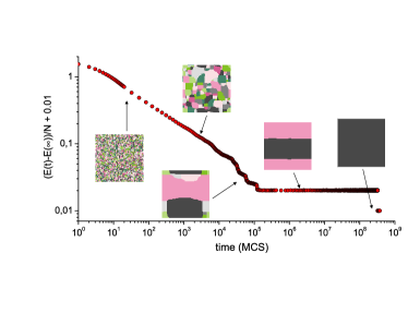
In order to compare the behavior of the average energy per spin $e(t)=\left<H\right>/N$ for different temperatures, we first introduce the relaxation function (or normalized excess of energy)

$$\phi_{E}(t)\equiv\frac{e(t)-e(\infty)}{e(0)-e(\infty)}$$ (5)

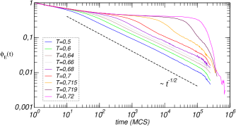
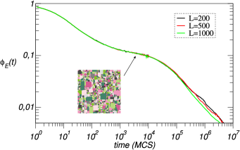
where $e(\infty)$ is the equilibrium energy. In Fig.1 we show the typical behavior of $\phi_{E}(t)$ for $L=300$ and temperatures between $0.72$ and $0.5$ ($T_{c}=0.7213\ldots$). For temperatures close enough to $T_{c}$ ($0.715<T<T_{c}$) we see that the system clearly stuck in a high energy metaestable state. Close examination of different quantities in the metastable state show that this corresponds to a disordered (i.e., paramagnetic) one and hence it is directly related to the first order nature of the transition. Moreover, we found evidences that in this regime relaxation is dominated by nucleation mechanisms, but the details of that analysis will be presented in a forthcoming publication. For temperatures $T<0.715$ we see that the metastable plateau disappears and the relaxation function decays (after a short transient) for all temperatures as $\phi_{E}(t)\sim t^{-1/2}$. Since the excess of energy respect to the equilibrium state in a domain growth process is given by the average energy of the domain walls, a simple calculation shows that $\phi_{E}(t)\sim 1/l(t)$, $l(t)$ being the average linear domain size. Hence, the behavior of Fig.1 is consistent with the LAC law. As we will show later, the finite size scaling properties of the average typical equilibration time in this temperature range are also consistent with the LAC law.

Figure 2: (Color on-line) Equilibration time probability distribution $P(\tau)$ for $L=100$ and $q=9$. (a) Temperatures ranging from $T=0.4$ (top) to $T=0.719$ (bottom); (b) temperatures ranging from $T=0.3$ (left) to $T=0.09$ (right).

III.1 Relaxation at intermediate temperatures and blocked states: characterization and scaling

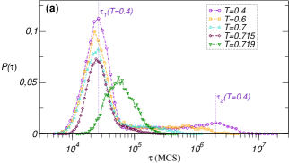
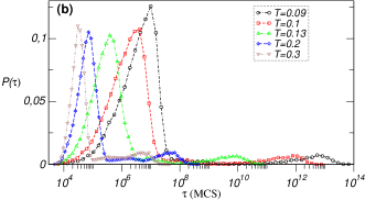
In Fig.2 we see the typical behavior of $P(\tau)$ for an intermediate size ($L=100$) and different temperature ranges. The different dynamical regimes can be already appreciated in this figure. Close enough to $T_{c}$ ($T=0.719$ in Fig.2a) $P(\tau)$ exhibit a well defined peak centered at a characteristic time $\tau_{nucl}\sim 10^{5}$ MCS, which is associated to a nucleation based relaxation mechanism already mentioned. As the temperature decreases below some temperature $0.715<T_{n}<T_{c}$, this peak is suddenly replaced by another one centered at a characteristic value $\tau_{1}$, which is about one order of magnitude smaller of $\tau_{nucl}$ and remains almost independent of the temperature in the range $0.3<T<0.715$; in the temperature range $0<T\leq 0.2$ (see Fig.2b), $\tau_{1}$ exhibit a strong temperature dependency. For temperatures smaller than (but close to) $T_{n}$ (see Fig.2a), $P(\tau)$ develops a long right tail; for temperatures $T<T^{*}\approx 0.6$ the tail becomes a distinct peak centered at a new characteristic time $\tau_{2}$, which increases exponentially as the temperature decreases. This behavior indicates the existence of two distinct phenomena affecting the relaxation at different time scales, where $T^{*}$ acts as a reference temperature signaling the time scales separation crossover point. The temperature behavior of $\tau_{1}$ and $\tau_{2}$ is summarized in the Arrhenius plot of Fig.3 .

Figure 3: (Color on-line) Characteristic relaxation times $\tau_{1}$ and $\tau_{2}$ vs. $1/T$ for $L=100$ and $q=9$; the same qualitative behaviors are observed for other system sizes. The continuous lines are a guide to the eye.

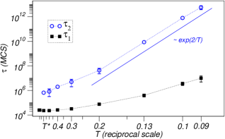
We will show that $\tau_{1}$ is associated with simple coarsening processes that follow LAC law for all times, while $\tau_{2}$ is associated to processes in which the system gets stuck in striped metastable states, composed by two ferromagnetic states whose walls are parallel to coordinate axis, as shown in the example of Fig.4. Those type of metastable states have been already observed in the two dimensional Ising model ($q=2$) at zero temperature, where they become frozenLipowski (1999); Spirin et al. (2001a, b); Sundaramurthy and Stein (2005); de Oliveira et al. (2006). At finite temperature, striped states perform a random parallel movement in the direction perpendicular to the walls. Hence, in a finite system those states relax to equilibrium when both walls collapse. Spirin, Kaprivsky and RednerSpirin et al. (2001a) showed that the basic mechanism for the parallel movement of a straight domain wall is the creation of a “dent”, that is, the flip of one of the spins adjacent to the wall. Since after flipping the spin its neighbors can flip without energy cost, the energy barrier for the creation of a dent is $2$ (in units of the coupling constant $J$) for the $q=2$ Potts model (or $4$ for the Ising model). For $q>2$ the energy cost of any other movement (including a flipping to a third color different from those of the domains) is larger. Hence, once the striped state is reached, the time needed to relax should be basically independent of $q$ and this is consistent with the Arrhenius behavior $\tau_{2}\sim e^{2/T}$ observed in Fig.3.

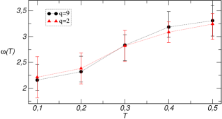
From Fig.3 we can notice also that, for a wide range of temperatures $T<T_{n}$ (approximately down to $T\approx 0.2$) $\tau_{1}$ remains almost independent of $T$, consistently with a simple coarsening behavior; at lower temperatures we see a crossover into an activated behavior, that will be analyzed later.

Figure 4: (Color on-line) Energy per spin as a function of time and typical spin configurations in one realization of the stochastic noise, when the system gets stuck in a striped configuration ($L=200$, $q=9$ and $T=0.2$). The different colors codify different spin values $s_{i}=1,\ldots,9$

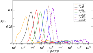
A deeper understanding of the mechanisms involved in the relaxation can be obtained from the finite size scaling of the different quantities involved. In Fig.5 we show the typical behavior of $P(\tau)$ for different system sizes at a fixed temperature $T=0.2$. The first thing we note is that the two-peak structure remains in the large $L$ limit. Moreover, the ratio between the areas below both peaks becomes constant in such limit. The same property is observed for temperatures up to $T^{*}$. We will analyze this in more detail at the end of this section. Let us now consider the finite size scaling of the relaxation times.

Figure 5: (Color on-line) Equilibration time probability distribution $P(\tau)$ for $T=0.2$, $q=9$ and system sizes ranging from $L=15$ (left) to $L=500$ (right).

From Fig.6 we see that $\tau_{1}\sim L^{2}$ for a wide range of temperatures, both above and below $T^{*}$. This is also consistent with a simple coarsening process, in which equilibration will be attained once $l(\tau)\sim\tau^{1/2}\sim L$.

Figure 6: (Color on-line) Characteristic relaxation time $\tau_{1}$ vs $L$ for $q=9$ and different temperatures; dotted lines are a guide to the eye.

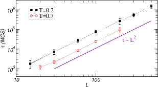
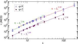
Let us now analyze the finite size scaling of $\tau_{2}$. Spirin, Kaprivsky and RednerSpirin et al. (2001a) suggested that, at low enough temperatures, the movement of a flat interface will be dominated by processes involving a single dent creation; once the dent is created it performs a random walk, until either the dent disappears or it covers the whole line, where the typical time needed for the last event scales asSpirin et al. (2001a) $L$. This mechanism leads to a random walk movement of both interfaces, so there must be typically $L^{2}$ such hopping events for the interfaces to meet and therefore the relaxation time should scale asSpirin et al. (2001a) $L^{3}$. However, this argument only works for small system sizes. Once a dent is created, the probability of creation of new dents along the interface, before the dent covers the line, increases with the system size; therefore, the typical time for a one-site hoping event of an entire interface should increase slower than linearly with $L$ and $\tau_{2}$ slower than $L^{3}$. This can be appreciated in the clear crossover from $\tau_{2}\sim L^{3}$ to $\tau_{2}\sim L^{\omega}$ with $\omega<3$ around $L=15$, observed in Fig.7, both for $q=2$ and $q=9$ (the same effect is observed for any temperature $T\leq 0.2$). Striped states appear for temperatures up to $T^{*}$, but the the walls movements are no longer dominated by one-site hopping events for $T>0.2$; instead of that, a direct inspection of the spin configuration during relaxation shows that, at temperatures close to $T^{*}$ the movements of the domain walls resemble (for large system sizes) that of elastic lines subjected to a random noise. Hence, the temperature dependence of $\tau_{2}$ departs from the $e^{2/T}$ behavior, as can be seen from Fig.3. However, the finite size scaling $\tau_{2}\sim L^{\omega}$ still holds for temperatures up to $T^{*}$, where the exponent $\omega$ displays a marked increase with the temperature, reaching values slightly larger than $3$ as $T$ approaches $T^{*}$ (see Fig.8). Those values of the exponent can be understood through the following argument. Suppose that each line behaves as a chain of $L$ unit masses joined by springs, constrained to move along the direction perpendicular to the wall and subjected to independent white noise. By solving the corresponding Langevin equations in the overdamped limit, a simple calculation shows that the distance between the centers of mass of both chains performs a Brownian motion with an effective diffusion coefficient that scales as $D\sim L^{-1}$. Since the distance between walls is of the order of $L$, this implies that the typical time needed for the walls to encounter should scale approximately as $L^{3}$. For $q=2$ LipowskiLipowski (1999) has shown that this scaling holds even for relatively large values of the temperature $T/T_{c}(2)\approx 0.8$. The results of Fig.8 suggest that the scaling properties of $\tau_{2}$ are independent of $q$, showing that large degeneracies in the ground state have no influence in this relaxation process.

Figure 7: (Color on-line) Characteristic relaxation time $\tau_{2}$ vs $L$ for $T=0.2$ and different values of $q$. The dashed lines correspond to linear fittings.

Figure 8: (Color on-line) Finite size scaling exponent $\omega$ of the characteristic relaxation time $\tau_{2}$ as a function of $T$ for different values of $q$; dotted lines are a guide to the eye.

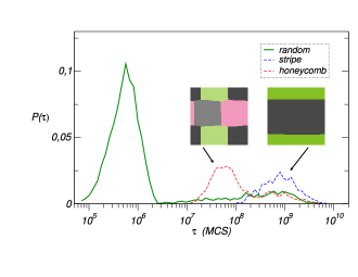
Let us return to the equilibration time probability distribution $P(\tau)$. Another salient feature of this distribution for temperatures $T<T^{*}$ is that the right peak broadens for large system sizes. To show this we redraw $P(\tau)$ for $L=300$ and $T=0.2$ in Fig.9 (full line). A careful inspection of individual processes shows that, such broad peak is actually associated with two different types of metastable configurations: the striped ones already described and honeycomb like structures; the latter are composed macroscopic six-sided irregular polygonal domains of different colors (see inset of Fig.9), where the angles between domain walls at the three-fold edges fluctuate around $120^{o}$. Those states are in agreement with Lifshitz predictionLifshitz (1962) for $q\geq 3$ and we shall call them Lifshitz states. By a calculation of the equilibration time starting directly from the Lifshitz and striped states, we verified that the broad peak of $P(\tau)$ is actually a superposition of two peaks, each one with its own distinctive maximum at characteristic times $\tau_{2}$, for the striped states, and $\tau_{3}$ for the Lifshitz ones (see Fig.9). Lifshitz states are only detectable for system sizes $L\geq 100$. Actually, isolated three-fold vertex between flat domain walls of the type predicted by LifshitzLifshitz (1962) also appear for smaller system sizes, but complete honeycomb-like structures can be stabilized during detectable time scales (i.e., larger than the characteristic coarsening time scales) only for large enough system sizes. To determine the scaling properties of $\tau_{3}$, we calculated the escape time probability distribution starting from the closest configuration to a Lifshitz state, that is, from an almost perfect four-colored honeycomb configuration (commensurability with the system size does not always allow a perfect honeycomb structure) for different values of $L$ and $T$; we show an example in Fig.9. We verified that the system quickly relaxes from that configuration into a Lifshitz state, from which it can either relax directly to the equilibrium state or pass first to a striped state, giving rise to a second peak in the corresponding probability distribution (see Fig.9). For completeness, we also calculated the escape time probability distribution starting from a perfect two-domains striped state; the result is also shown in Fig.9.

Figure 9: (Color on-line) Equilibration time probability distribution $P(\tau)$ starting from different initial configurations (arbitrary normalization) for $L=300$, $T=0.2$. The inset images show typical blocked spin configurations at the corresponding times.

Figure 10: Characteristic relaxation time $\tau_{3}$ vs temperature for $q=9$ and $L=100$; the continuous line is a guide to the eye.

Figure 11: (Color on-line) Basic relaxation mechanism of a Lifshitz state at low temperatures. The circle in (b) marks the creation of a dent in the vertex of (a), by flipping a spin from 2 $\rightarrow 3$. Circles in (c) and (d) exemplify spins that can flip without energy cost along the three converging walls. The whole process may lead to the hopping of the whole structure (vertex plus walls) and ultimately to the collapse of two vertex.

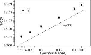
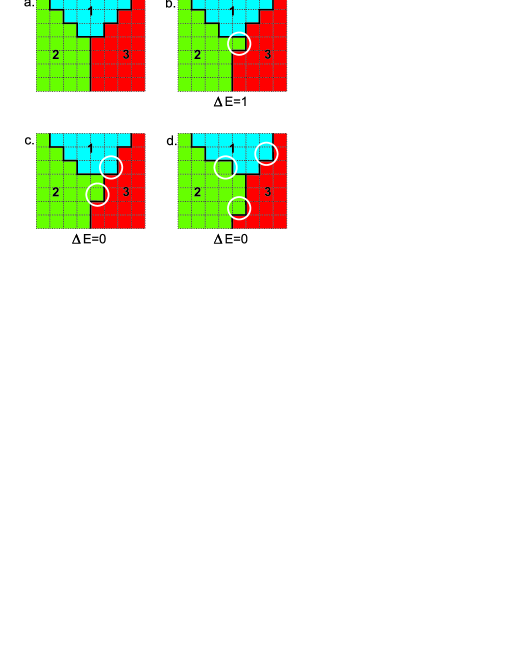
The temperature dependency of $\tau_{3}$ is shown in Fig.10, where we see that it displays a clear Arrhenius behavior with an activation barrier of height one, which is the minimum possible energy barrier associated with a single spin flip. This can be understood if we analyze the basic mechanisms behind the relaxation from Lifshitz states. We observed that Lifshitz states relax when two vertex of an hexagon edge collapse. A vertex movement, with the consequent displacement of the converging walls, occurs through a series of random hopping events. In Fig.11 we show an example of the hopping of a vertex one site to the right; one-site hopping events in the other directions follow a similar process with the same energy cost. The movement of a vertex starts with the creation of a dent, by flipping one of the spins located at the neighbor sites of the vertex, as depicted in Fig.11b. This movement has an energy cost of one unit. Once the dent is created, the neighbor spins at the three converging walls are free to flip without energy cost (see Figs.11c and 11d), generating a diffusive motion of the dent along the three lines, and may lead to the displacement of the whole lines. This hopping movement of the vertex ultimately leads to the collapse of two of them and the consequent disappearance of the Lifshitz state. The whole mechanism is completely similar to that described by Spirin, Kaprivsky and RednerSpirin et al. (2001a) in the case of a flat wall between two striped domains, except that the creation of a dent adjacent to a vertex has an energy cost of just one energy unit (instead of 2, as in the case of a dent in a flat interface), which explains the behavior of Fig.10. Since hexagonal domains in a Lifshitz state are macroscopic, the same finite size scaling arguments used by Spirin, Kaprivsky and RednerSpirin et al. (2001a) for the relaxation time apply in this case. Hence, one expect $\tau_{3}\sim L^{\omega}\;e^{1/T}$. For the system sizes available, we verified this scaling at low temperatures with an exponent $\omega\approx 3$, but we would expect this value to be reduced for larger system sizes, as in the case of striped states ($\tau_{2}$).

III.2 Probability of blocked states

We analized the probability $P_{b}(q)$ of getting stuck in a blocked state. We defined blocked states as those characterized by flat walls between domains. For $q\geq 3$ this includes Lifshitz and striped states. For $q=2$ the system can also get trapped in another type of blocked states, characterized by diagonal stripes, whose interfaces fluctuate without energy costSpirin et al. (2001b); we shall call them diagonal states. For $q\geq 3$ we did not observed diagonal states at finite temperatures. Although their presence for $q\geq 3$ with low probability cannot be excluded, probably they are replaced at finite temperature by the Lifshitz states.

From the previous calculations of $P(\tau)$ we could estimate $P_{b}(q)$ by defining for (for every value of $T$ and $L$) a threshold value $\tau_{t}(T,L)$, such that a single realization with $\tau>\tau_{t}$ is attributed to the presence of a blocked state; $\tau_{t}$ can be estimated as the first minimum of $P(\tau)$ located above $\tau_{1}$ (see for instance Fig.5). This procedure reduces the calculation of $P_{b}(q)$ to a binomial experiment. hence, a simple calculation shows that a sample size of $2000$ runs is enough to guarantee a statistical error smaller than $1\%$ in all cases, thus saving a lot of CPU time.

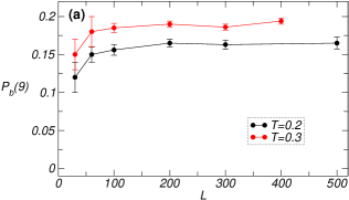
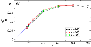
In Fig.12 we show the results for $q=9$. The main source of error in this calculation is the choice of $\tau_{t}$, which is not always evident, due to large fluctuations in the histograms for small sizes and very low temperatures; the error bars in Fig.12 were estimated by varying $\tau_{t}$. From Fig.12a we see that, at $T>0$, $P_{b}(9)$ saturates in a finite value for $L\geq 100$, indicating a finite probability in the limit $L\rightarrow\infty$. In Fig.12b we show the temperature dependency of the saturation value. We see that $P_{b}(9)$ goes to zero as $T\rightarrow 0$, consistently with the results of Spirin, Kaprivsky and RednerSpirin et al. (2001b).

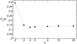
Next we analyzed the probability $P_{b}(q)$ as a function of $q$. The results are shown in Fig.13 for $T=0.15$ and values of $q$ ranging from $q=2$ up to $q=30$ . For $q=2$ and $T=0$ the probability of reaching a striped state isSpirin et al. (2001a); Fialkowski and Holyst (2005) $1/3$, while the probability of reaching a diagonal state isSpirin et al. (2001b) $\approx 0.04$. At $T=0.15$ we found the values $\approx 0.345$ and $\approx 0.045$ respectively, giving rise to the value $P_{b}(2)\approx 0.39$. The differences with the $T=0$ values are consistent with the enhancement of the probability at finite temperature, already observed for $q=9$.

For $q\geq 3$ the probability $P_{b}(q)$ falls down to a temperature dependent finite value, that is almost independent of $q$ and smaller than half of $P_{b}(2)$.

It is worth noting that Spirin, Kaprivsky and RednerSpirin et al. (2001b) reported another type of blocked states for $q=3$, characterized by both straight walls and diagonal walls, the latter fluctuating without energy cost; they call these states “blinkers”. We did not observe blinkers at finite temperature, at least for periodic boundary conditions. Although their existence with low probability cannot be excluded, probably they decay into Lifshitz states in time scales smaller than the characteristic Lifshitz relaxation times.

Figure 12: (Color online) Probability of getting stuck in a blocked state $P_{b}(q)$ for $q=9$: (a) as a function of $L$ for different temperatures; (b) as a function of $T$ for different sizes. The dashed line corresponds to a linear fitting of the points for $L=200$, giving an extrapolated value of $0.008\pm 0.01$ at $T=0$.

Figure 13: Probability of getting stuck in a blocked state $P_{b}(q)$ for $L=200$ and $T=0.15$.

III.3 Low temperatures relaxation: glassy states

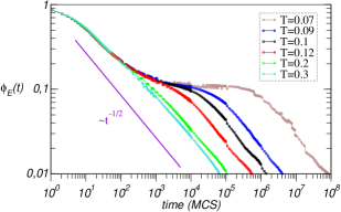
Let us now analyze the coarsening at very low temperatures. The increase of $\tau_{1}$ for temperatures $T<0.2$ observed in Fig.3 indicates that the normal coarsening is affected by some kind of activated process. The increase in this relaxation time is associated with the plateau displayed by the relaxation function in Fig.14. We found that this plateau appears below some characteristic temperature $0.1<T_{g}<0.2$ for $q=9$. This plateau corresponds to a disordered metastable state characterized by almost square–shaped domains with a wide distribution of sizes (see inset in Fig.15). That type of metastable state was previously reported for $q=7$ and it was identified as a glassy onePetri (2003); de Oliveira et al. (2004); Oliveira et al. (2004).These states are only present forde Berganza et al. (2007a) $q>4$. We verified that for $q=9$ the normal coarsening is always interrupted for $T<T_{g}$ and the system gets stuck in one of those glassy states, from which it relaxes through a complex sequence of activated jumps. This explains the exponential increase of $\tau_{1}$ observed in Fig.3 for $T<0.2$. Once the system relaxes from the glassy state, it can be either directly equilibrate or decay first in a blocked state.

In Fig.15 we show the typical behavior of relaxation function for $q=9$ at a fixed temperature $T<T_{g}$ and different system sizes. We see that the relaxation time ($\tau_{1}$) is size independent for $L>200$, which shows that the life time of the glassy states remains finite in the thermodynamic limit.

Figure 14: (Color on-line) Relaxation function for $q=9$, $L=200$ and different temperatures around $T_{g}$. Temperatures increase from right to left.

Figure 15: (Color on-line) Relaxation function for $q=9$, $T=0.1$ and different values of $L$. The inset shows a typical configuration of the glassy state associated with the plateau.

III.4 Boundary conditions

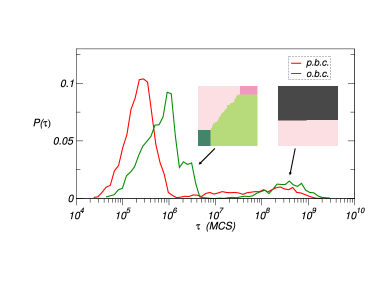
Finally, we analyzed the influence of the boundary conditions in the relaxation. To this end, we repeated some of the previous calculations using open boundary conditions. We found that the overall relaxation scenario found using periodic boundary conditions repeats qualitatively for open ones. Moreover, the relaxation time associated with striped configurations appears to be of the same order of magnitude of that corresponding to periodic boundary conditions. Although a more systematic study should be done to confirm that, it seems reasonable since the basic activated mechanisms here described should be still dominant in the case of open boundary conditions. In Fig.16 we show an example of the equilibration time probability distribution for $q=9$ and some typical blocked spin configurations. In this case, Lifshitz states are no longer composed only by hexagons for relatively small system sizes (due to the presence of the borders), but we see clearly the presence of stable three-colored vertex. Indeed, the observed configurations strongly resemble the blinking states reported in Ref.Spirin et al. (2001b).

Figure 16: (Color on-line) Equilibration time probability distribution $P(\tau)$ for $q=9$, $L=200$ and $T=0.2$, using periodic (p.b.c) and open (o.b.c) boundary conditions. The inset images show typical blocked spin configurations observed with o.p.c.

IV Summary and conclusions

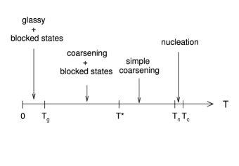
The main conclusions of this work are summarized in the scheme of Fig.17. After a quench from infinite temperature down to subcritical temperatures, the Potts model with single spin flip kinetics and periodic boundary conditions presents for $q>4$ different relaxational regimes, determined by different crossover characteristic temperatures. Close enough to the critical temperature, i.e., for $T_{n}<T<T_{c}$, relaxation is dominated by nucleation mechanisms. For intermediate temperatures $T^{*}<T<T_{n}$ the system crosses over into a simple coarsening dominated regime where LAC law $l(t)\sim t^{1/2}$ holds until full equilibration, for most of the realizations of the stochastic noise. For lower temperatures $T_{g}<T<T^{*}$ the normal coarsening process is interrupted when the system gets stuck into highly symmetric blocked configurations, composed by macroscopic ferromagnetic domains, namely, striped and Lifshitz states. In those cases, the dynamic becomes activated with characteristic energy barriers, which give rise to distinct time scales for the different process.

Figure 17: Dynamical regimes in the long term relaxation of the q-state Potts model with $q>4$, after a quench from infinite temperatures down to a sub–critical temperature $T$.

Concerning the role of temperature in the relaxation through blocked states, we found that it has a double effect: at short time scales it enhances the probability of reaching them (which is zero at $T=0$) and at long time scales it allows to escape from them through activation. At least for $q=9$, our simulations (for system sizes up to $L=500$) suggest that the probability of reaching a blocked state at finite temperatures remains finite when $L\rightarrow\infty$.

Striped states were previously found and characterized for the Ising model ($q=2$) at very low temperatures. We found that their influence in the relaxation process is relevant for any value of $q$ , even at relatively large values of $T$, but their occurrence probability is smaller for $q\geq 3$ than in the Ising case.

We found that the relaxation times associated with the blocked states present in general the finite size scaling behavior $\tau\sim L^{\omega}$, where the exponent $\omega$ depends on $T$, taking values between $2$ and $4$. Such values of the exponent make the associated time scales several orders of magnitude larger than those associated with a normal coarsening process (which scale as $L^{2}$) for large enough sizes, even at relatively large values of the temperature.

Lifshitz prediction have been recently verified in the phase separation dynamics of diblock copolymers (Cahn-Hillard model), in a 2D hexagonal substrateGomez et al. (2006). We verified that Lifshitz prediction also holds for the $q$ state Potts model with $q\geq 3$, even in a square lattice, if the system size is large enough. This strong finite size effects is probably due to the square symmetry of the lattice (large system sizes are required in order to the influence of the lattice to be faded out) and one should expect to be reduced in a lattice with three-fold symmetry (for instance, triangular).

At very low temperatures $T<T_{g}$ the system gets always trapped in glassy like metastable configurations whose life time is size–independent and diverge for $T\rightarrow\infty$. After relaxation from the glassy state, the system can again gets trapped in a blocked state. Even when the glassy states do not dominate the relaxation at long enough time scales, a complete description of the relaxation dynamics cannot exclude their existence and therefore they deserve further investigations.

Finally, we verified that the whole qualitative relaxation scenario appears both for periodic and open boundary conditions, although the finite size scaling of the relaxation times may differ in both cases.

Fruitful discussions with M. Ibañez de Berganza, F. A. Tamarit and C. B. Budde are acknowledged. This work was partially supported by grants from CONICET (Argentina), SeCyT, Universidad Nacional de Córdoba (Argentina), FONCyT grant PICT-2005 33305 (Argentina) and ICTP grant NET-61 (Italy).

References

- Lifshitz (1962) I. Lifshitz, Sov. Phys. JEPT 15, 939 (1962).
- Safran (1981) S. A. Safran, Phys. Rev. Lett. 46, 1581 (1981).
- Vinals and Grant (1987) J. Vinals and M. Grant, Phys. Rev. B 36, 7036 (1987).
- Grest et al. (1988) G. S. Grest, M. P. Anderson, and D. J. Srolovitz, Phys. Rev. B 38, 4752 (1988).
- Kumar et al. (1987) S. Kumar, J. D. Gunton, and K. K. Kaski, Phys. Rev. B 35, 8517 (1987).
- Sire and Majumdar (1995) C. Sire and S. N. Majumdar, Phys. Rev. Lett. 74, 4321 (1995).
- Wu (1982) F. Y. Wu, Rev. Mod. Phys. 54, 235 (1982).
- Petri (2003) A. Petri, Braz. Journ. Phys. 33, 521 (2003).
- de Oliveira et al. (2004) M. de Oliveira, A. Petri, and T. Tomé, Physica A 342, 97 (2004).
- Oliveira et al. (2004) M. Oliveira, A. Petri, and T. Tomé, Europhys. Lett. 65, 20 (2004).
- de Berganza et al. (2007a) M. I. de Berganza, V. Loretto, and A. Petri, Phylosophical Magazine 87, 779 (2007a).
- de Berganza et al. (2007b) M. I. de Berganza, E. E. Ferrero, S. A. Cannas, V. Loretto, and A. Petri, Eur. Phys. J. Special Topics 143, 273 (2007b).
- Bortz et al. (1975) A. Bortz, M. Kalos, and J. Lebowitz, J. Comp. Phys. 17, 10 (1975).
- Novotny (1995) M. A. Novotny, Phys. Rev. Lett. 74, 1 (1995).
- Lipowski (1999) A. Lipowski, Physica A 268, 6 (1999).
- Spirin et al. (2001a) V. Spirin, P. L. Krapivsky, and S. Redner, Phys. Rev. E 63, 036118 (2001a).
- Spirin et al. (2001b) V. Spirin, P. L. Krapivsky, and S. Redner, Phys. Rev. E 65, 016119 (2001b).
- Sundaramurthy and Stein (2005) P. Sundaramurthy and D. L. Stein, J. Phys. A: Math. Gen. 38, 349 (2005).
- de Oliveira et al. (2006) P. M. C. de Oliveira, C. M. Newman, V. Sidoravicious, and D. L. Stein, J. Phys. A: Math. Gen. 39, 6841 (2006).
- Glazier et al. (1990) J. A. Glazier, M. P. Anderson, and G. S. Grest, Phylosophical Magazine B 62, 615 (1990).
- Glazier and Weaire (1992) J. A. Glazier and D. Weaire, J. Phys: Condens. Matter 4, 1867 (1992).
- Weaire and Glazier (1992) D. Weaire and J. A. Glazier, Materials Science Forum 94-96, 27 (1992).
- Thomas et al. (2006) G. L. Thomas, R. M. C. de Almeida, and F. Graner, Phys. rev. E 74, 021407 (2006).
- Graner and Glazier (1992) F. Graner and J. A. Glazier, Phys. Rev. Lett. 69, 2013 (1992).
- Kihara et al. (1954) T. Kihara, Y. Midzuno, and T. Shizume, J. Phys. Soc. Japan. 9, 681 (1954).
- Fialkowski and Holyst (2005) M. Fialkowski and R. Holyst, Eur. Phys. J. E 16, 247 (2005).
- Gomez et al. (2006) L. R. Gomez, E. M. Valles, and D. A. Vega, Phys. Rev. Lett. 97, 188302 (2006).