Magnetar-energized supernova explosions and GRB-jets

Abstract

In this paper we report on the early evolution of a core-collapse supernova explosion following the birth of a magnetar with the dipolar magnetic field of $B=10^{15}$G and the rotational period of $2$ms, which was studied by means of axisymmetric general relativistic MHD simulations. In this study we use realistic EOS and take into account the cooling and heating associated with emission, absorption, annihilation, and scattering of neutrinos, the neutrino transport is treated in the optically-thin regime. The supernova explosion is initiated via introducing into the initial solution the “radiation bubble”, whose total thermal energy is comparable with the typical energy of supernova ejecta. The numerical models exhibit highly collimated magnetically-driven jets very early on. The jets are super-Alfvénic but remain sub-fast until the end of the simulations (t=0.2s). The power released in the jets is about $3\times 10^{50}$erg/s which implies the spin-down time of $\simeq 37$s. The total rotational energy of the magnetar, $E\simeq 10^{52}$erg, is sufficient to drive a hypernova but it is not clear as to how large a fraction of this energy can be transfered to the stellar ejecta. Given the observed propagation speed of the jets, $v_{p}\simeq 0.17c$, they are expected to traverse the progenitor in few seconds and after this most of the released rotational energy would be simply carried away by these jets into the surrounding space. 3-dimensional effects such as the kink mode instability may reduce the jet propagation speed and increase the amount of energy transferred by the jets to the supernova ejecta. Our results provide the first more or less self-consistent numerical model of a central engine capable of producing, in the supernova setting and on a long-term basis, collimated jets with sufficient power to explain long duration GRBs and their afterglows. Although the flow speed of our jets is relatively low, only $v_{j}\simeq 0.5c$, the cooling of proto-neutron star will eventually result in much higher magnetization of its magnetosphere and ultra-relativistic asymptotic speeds of the jets. Given the relatively long cooling time-scale we still expect the jets to be only weakly relativistic by the time of break out. This leads to a model of GRB jets with systematic longitudinal variation of Lorentz factor which may have specific observational signatures both in the prompt and the afterglow emission. The simulations also reveal quasi-periodic ejection of plasma clouds into the jet on a time-scale of 20ms related to the large-scale global oscillation of magnetar’s magnetosphere caused by the opening-closing of the dead zone field lines. These kind of central engine variability may be partly responsible for the internal shocks of GRB jets and the short-time variability of their gamma-ray emission.

1 Introduction

After decades of intensive research the exact mechanism of core-collapse supernovae (SNe) still remains a mystery. It is widely believed that the explosion is driven by neutrinos emitted by the proto-neutron star (PNS) formed as the result of the collapse [Bethe 1990]. However, the attempts to reproduce core-collapse SNe in computer simulations have encountered severe problems. The reason for the failures becomes more or less clear when one compares the total energy radiated in the form of neutrinos, $\simeq 10^{53}$erg, with the typical energy of supernovae, $\simeq 10^{51}$erg. This tells us that in order to obtain a reliable answer the computational error in the energy budget has to be below $1\%$, which a is very demanding condition. The neutrino transport, of six different species, has to be treated with great accuracy including the processes effecting heating and cooling rates.

The alternative magnetic mechanism of core-collapse SNe has been around for a while, first proposed by Bisnovatyi-Kogan[Bisnovatyi-Kogan 1970] and LeBlanc & Wilson[LeBlanc & Wilson 1970], whose numerical simulations were miles ahead of their time. For three decades this mechanism was not taken seriously and only occasionally efforts were made to develop it further [Bisnovatyi-Kogan 1976, Meier et al. 1976, Symbalisty 1984]. Now it is experiencing “renaissance” [Wheeler et al. 2000, Wheeler et al. 2002, Akiyama et al. 2003, Yamada & Sawai 2004, Kotake et al. 2004, Mizuno et al. 2004, Takiwaki et al. 2004, Ardeljan et al. 2005, Akiyama & Wheeler 2005, Proga 2005, Moiseenko et al. 2006, Obergaulinger 2006, Shibata et al. 2006, Masada et al. 2007, Nagataki et al. 2007, Burrows et al. 2007], thanks to the slow and difficult progress of the neutrino models of SNe, the development of robust numerical methods for MHD, the accumulated evidence for asphericity of supernovae [Khokhlov et al. 1999, Wang et al. 2002, Wang et al. 2003] , the high collimation of flows associated with GRBs (e.g. Piran 2005a,b) and the increasing popularity of the magnetic mechanism for the origin of other astrophysical jets. The results show that magnetic field can facilitate explosions of standard power and even more powerful explosions provided the magnetic field is sufficiently strong.

The energy of high-velocity supernovae or hypernovae (HNe) exceeds that of normal core-collapse supernovae by about ten times (e.g. Nomoto et al. 2004). The few SNe that have been reliably identified with GRBs are all HNe. Although, the statistics is very poor and is subject to observational bias towards most powerful and hence brightest events, the connection between HNe and GRBs is widely accepted. The physical mechanism of HNe is not established and there is no shortage of competing theoretical models. The most popular one, the collapsar model, relates HNe with collapse of massive rapidly rotating stars [MacFadyen & Woosley 1999]. In this model, the stellar core collapses straight into a black hole (which used to be considered as an indication of “failed” supernova explosion) but the stellar envelope does not and forms a hyper-accreting disk around the hole. The energy released in the disk can be very large, sufficient to drive HN and GRB, but the way it is transferred to the supernova ejecta and the GRB jets remains to be determined. It is widely assumed that GRB jets are powered by the energy released in the funnel region of the disk via annihilation of neutrinos [Ruffert & Janka 1999, Narayan et al. 2001]. However, taking into account opacity in the inner regions of the disk significantly reduces the efficiency of this mechanism [Di Matteo et al. 2002, Nagataki et al. 2007]. Alternatively, as it has been suggested by many authors, the GRB-jets in the collapsar scenarion can be powered via magnetic mechanism tapping the rotational energy of the black hole and/or the accretion disk (e.g. Lyutikov & Blandford 2003, Vlahakis & Konigl 2003, Proga et al., 2003).

The energy of HNe ejecta is of the same magnitude as the rotational energy of a neutron star (NS) with very short period of rotation, 1-2 milliseconds. This energy can be released via magnetic braking within a very short period of time, from few seconds to few hundreds of a second, provided the magnetic field is very strong, of order $B_{\mbox{\tiny NS}}\simeq 10^{15}$G [Thompson 2006, Bucciantini et al. 2006]. This value is three orders of magnitude above the typical strength of magnetic field of normal neutron stars and would be considered a huge over-stretch not so long time ago. However, the identification of Soft Gamma Ray Repeaters and X-ray Anomalous Pulsars with magnetars, neutron stars with magnetic field $B_{\mbox{\tiny NS}}\simeq 10^{14}-10^{15}$G [Thompson & Duncan 1995, Woods & Thompson 2004], shows that the magnetar model may be a viable alternative to the collapsar model of HNe as well as GRBs [Usov 1992, Thompson et al. 2004, Thompson 2006, Metzger et al. 2007, Uzdensky & MacFadyen 2006].

The origin of magnetar’s magnetic field is still debated. One possibility is the generation of unusually strong magnetic field in convective cores of some pre-supernova stars. During the core collapse the poloidal field is amplified like $\propto r^{-2}$ and in order to reach the required $B_{\mbox{\tiny NS}}\simeq 10^{15}$G after the collapse the original field in the core, on the scale of $~{}10^{3}$km, should be of order $B_{\mbox{\tiny C}}\simeq 10^{11}$G. The collapse of magnetized rotating stellar cores has been studied by many groups. The general conclusion from the latest parameter studies is that only for $B_{\mbox{\tiny C}}\geq 10^{11}$G the magnetic field is strong enough to influence the dynamics of supernovae explosions [Obergaulinger 2006, Burrows et al. 2007]. The key feature of these explosions is strong differential rotation and generation of toroidal magnetic field whose pressure actually drives the explosion. The hoop stress of this field also ensures anisotropy of the explosion - it is more powerful along the rotational axis.

On the other hand, the super-strong magnetic field of magnetars could be generated via $\alpha$-$\Omega$-dynamo in the convective PNS [Duncan & Thompson 1992, Thompson & Duncan 1993]. In this theory the strength of saturated field strongly depends on the rotational period - shorter period leading to stronger field. In order to generate the dipolar field of $B_{\mbox{\tiny NS}}\simeq 10^{15}$G the period of PNS should be very short, not much higher than few milliseconds [Duncan & Thompson 1992]. Thus, this theory unites both basic conditions required to produce a hypernova in the magnetar model, rapid rotation and super-strong magnetic field, in one. On the downside, the PNS is no longer magnetically coupled to the envelope and the transfer of its rotational energy to the stellar envelope is more problematic. Turbulence required for the magnetic dynamo action can also be generated via the magneto-rotational instability (MRI, Balbus & Hawley,1991). Calculations based on the linear theory show that in the supernova context strong saturation field can be reached very quickly on the time scale of only several tens of rotational periods [Akiyama et al. 2003].

Thompson et al.[Thompson et al. 2004] proposed a model of magnetically driven HN explosions and GRB where the usual delayed neutrino-driven mechanism plays the role of bomb detonator. The neutrino-driven blast creates a rarefaction around the newly-born magnetar, its magnetosphere expands and eventually develops a magnetically driven pulsar wind (PW). This wind acts as a piston on the expanding supernova envelope, that is the layer of compressed stellar material behind the supernova shock, and energizes it beyond the level of normal SN.

Metzger et al.[Metzger et al. 2007] generalized the 1D model of equatorial magnetically-driven wind by Weber & Davis[Weber & Davis 1967] to fit the conditions of PNS. Axisymmetric magnetized winds of magnetars with various degree of mass loading have been studied in Bucciantini et al.[Bucciantini et al. 2006] via 2D numerical simulations. They concluded that during the initial phase (Kelvin-Helmholtz timescale) when the wind is already magnetically-driven but still non-relativistic the rotational energy loss rate is $L\simeq 4\times 10^{51}B_{15}^{2}P_{1}^{-5/3}$erg/s, where $B_{15}$ is the magnetic field of the PNS in $10^{15}$G and $P_{1}$ is its period in milliseconds. Bucciantini et al.[Bucciantini et al. 2007a] applied the model of pulsar wind nebula (PWN) by Begelman & Li [Begelman 1992] to study the late phases of hypernova explosion, $t>1$s. They used the thin-shell approximation to describe the dynamics of the supernova shock driven by the anisotropic pressure of the magnetized bubble, “baby pulsar wind nebula”, created inside the exploding star by the magnetar wind. They concluded that when the magnetic energy in the bubble exceeds $\simeq 20\%$ of the thermal energy the shell expansion proceeds in a highly anisotropic fashion and eventually an axial channel is created inside the stellar envelope. They proposed that later this channel collimates the ultra-relativistic wind from cooled magnetars into a pair of GRB jets. In the follow up paper [Bucciantini et al. 2007b] they studied the interaction of the super-fast magnetar wind with the supernova envelope via fully relativistic MHD simulations and arrived to similar conclusions. For the wind model to become applicable the size of the “central cavity” must exceed, and likely many times, that of the fast surface as found in the unconfined case. Prior to this one would expect a somewhat different dynamics.

The most pessimistic possibility is a rigidly rotating magnetosphere in which case no extraction of rotational energy takes place. However, the theory of relativity places a upper limit on the size of such a magnetosphere. Indeed, the magnetosphere whose size exceeds the light cylinder (LC) radius cannot be rigidly rotating as this would imply superluminal motion of magnetospheric plasma and should become differentially rotating. This limit is particularly relevant for the magnetospheres of millisecond pulsars as the radius of LC, $R_{\mbox{\tiny LC}}\simeq 50P_{1}$ km, is only few times the radius of the star itself. Once the differential rotation sets up it amplifies the toroidal field, the magnetic pressure grows and promotes further expansion of the magnetosphere. Uzdensky & MacFadyen[Uzdensky & MacFadyen 2006] suggested that this factor along can explain supernova explosions but they did not elaborate ways to achieve the initial expansion beyond LC. Moreover, they assumed low mass loading of magnetic field lines, more suitable for NS than hot proto-NS, and concluded that the magnetospheric plasma will exhibit ultra-relativistic rotation in the equatorial plane. In any case, this argument suggests that the magnetic braking should begin to operate at the very early stages of the “detonated” magnetically-driven explosions, well before the central cavity expands beyond the fast surface of unconfined magnetar wind and this may to have important implications for their later development.

In this paper we describe an attempt to explore the early phase ($t\leq 1$s) of such explosions via axisymmetric General Relativistic MHD simulations. Our main goals are to study the basic dynamics of this phase, to determine the spin-down power, and to assess the implications for the later evolution. We use an upwind conservative scheme that based on a linear Riemann solver and uses the constrained transport method to evolve the magnetic field. The details of this numerical method and various tests are described in Komissarov[Komissarov 1999, Komissarov 2004b, Komissarov 2006]. In Sec.2 we describe the details of numerical experiments, including initial and boundary conditions, Sec.3 describes the results of simulations, and in Sec.4 we discuss their implications for the model of magnetar-driven supernovae explosions and GRB jets. Our conclusions are listed in Sec.5.

2 Simulation Setup

The ultimate hypernovae/supernovae simulations should trace all phases the stellar explosions, the onset of core collapse, core bounce, delayed explosion, generation of magnetic field, formation of magnetic cavity, and break out of magnetically-driven jets. Unfortunately this is still beyond our current capabilities and we have to make some simplifications. Here we start our simulations from the point when strong magnetic field has just appeared from surface of already formed PNS. To account for the previous stages of the explosion we assume that PNS is surrounded by a ”radiation bubble” with a large amount of energy deposited by neutrino in form of heat. The bubble is surrounded by the collapsing stellar envelope.

The gravitational attraction of PNS is introduced via Schwarzschild metric in Boyer-Lindquist coordinates, $\{\phi,r,\theta\}$. The two-dimensional computational domain is $(r_{0}<r<r_{1})\times(0<\theta<\pi)$, where $r_{0}$ corresponds to the radius of PNS and $r_{1}=10^{4}$km. The total mass within the domain is small compared to the mass of PNS that allows us to ignore its self-gravity. The grid is uniform in $\theta$ where it has 200 cells and almost uniform in $\log(r)$ where it has 430 cells, the linear cell size being the same in both directions.

2.1 PNS

The evolution of a non-rotating proto-neutron star of mass $M=1.4M_{\sun}$ have been studied in details by Burrows & Lattimer [Burrows & Lattimer 1986]. According to this study the deleptonization time-scale is rather long, it takes around 5 seconds before half the leptons inside $M(r)<0.5M$ are lost. However, the contraction time-scale is much shorter - it takes only $\simeq 250$ms for the star radius to decrease down to $\simeq 15$km (see fig.5 in Burrows & Lattimer, 1986). Using these results we fix the mass and radius of PNS to $M=1.4M_{\sun}$ and $r_{0}=15$km respectively, and we choose the rotation period to be $P=2$ms. To set the boundary conditions on the PNS surface we utilize the results of high resolution 1D numerical models of PNS winds [Thompson et al. 2001, Metzger et al. 2007]. The gas temperature of “ghost cells” is to $T_{0}=4$ MeV, which is typical for a hot newly-born PNS, and their density is $\rho_{0}=3\times 10^{9}\mbox{g}\mbox{cm}^{-3}$. This density corresponds to the interface between the very thin exponential atmosphere of PNS and its wind. The initial magnetic field is purely poloidal with the azimuthal component of vector potential

$$A_{\phi}=f(r)\frac{B_{0}r_{0}^{3}}{2r}\sin^{2}\theta,$$ (1)

where

$$f(r)=\left\{\begin{array}[]{rcl}1-((r-r_{0})/(r_{c}-r_{0}))^{2}&\mbox{if}&r<r_{c}\\ 0&\mbox{if}&r>r_{c},\end{array}\right.$$ (2)

$B_{0}=10^{15}$G and $r_{c}=1.8r_{0}$. For $f(r)=1$ equation 1 describes magnetic dipole of strength $B_{0}$ at $r=r_{0}$, $\theta=0$. The masking function (2) “moves” the magnetic field lines inside the sphere of radius $r_{c}$ without changing the magnetic flux distribution over the PNS surface. This distribution is preserved for the whole duration of simulations. The radial velocity of ghost cells is set to zero and the mass outflow through the boundary is found via solving the Riemann problem at the boundary interface.

We assume that neutrino luminosity in each species is given by the black body formula

$$L_{\nu}=1.20\times 10^{26}\pi r_{0}^{2}c\left(\frac{T_{0}}{1\mbox{MeV}}\right)^{4}\frac{\mbox{erg}}{\mbox{s}}\simeq 6.5\times 10^{51}\frac{\mbox{erg}}{\mbox{s}}$$ (3)

and that the mean neutrino energy is $e_{\nu}=3.15\,T_{0}=12.6$ MeV. This oversimplification is unlikely to have a strong effect on the largely magnetically driven outflows from PNS.

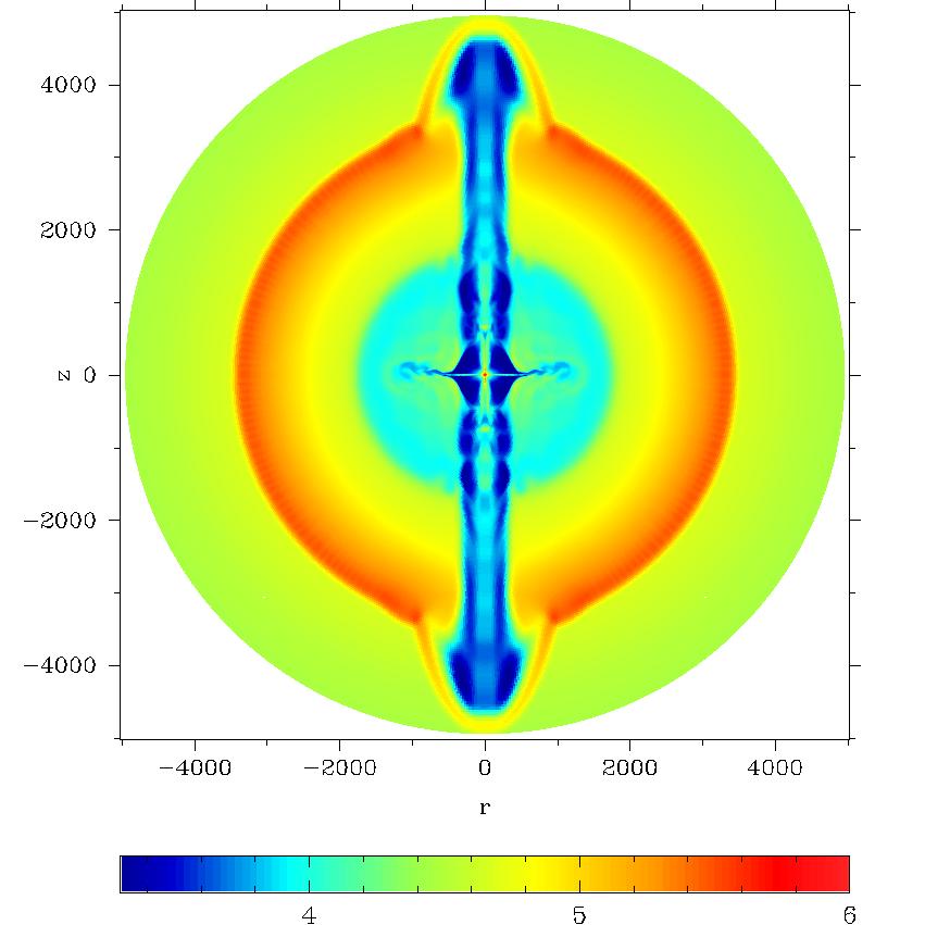
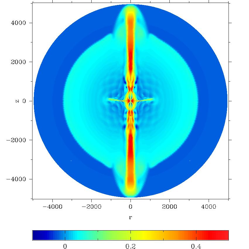
Figure 1: Model A at time $t\simeq 200$ ms. Left panel: $log_{10}\rho$ measured in $\mbox{g~{}cm}^{-3}$. Right panel: Radial velocity, $v^{r}/c$. The unit length in all figures in this paper is ${\cal L}=GM/c^{2}\simeq 2$km. The dynamic range of colour plots does not always reflect the full range of variation of the represented quantity but is rather selected to make more revealing images.

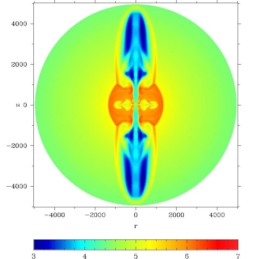
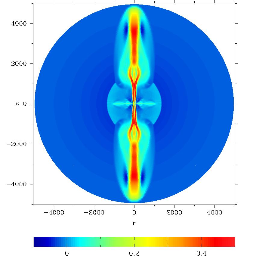
Figure 2: Same as in figure 1 but for model B at $t\simeq 200$ ms.

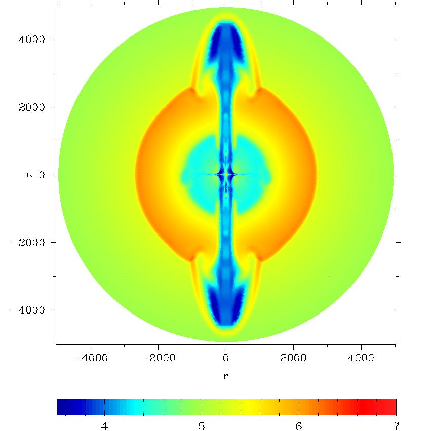
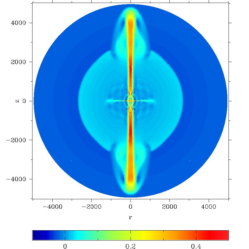
Figure 3: Same as in figures 1,2 but for model C at $t\simeq 277$ ms.

2.2 Collapsing star

Here we adopt the simple free-fall model by Bethe [Bethe 1990]. According to this model the radial velocity is

$$v^{r}_{\mbox{ff}}=(2GM/r)^{1/2},$$ (4)

and the density is

$$\rho=C_{1}\times 10^{7}\left(\frac{t_{s}}{1\mbox{~{}s}}\right)^{-1}\left(\frac{r}{10^{7}\mbox{cm}}\right)^{-3/2}\mbox{g~{}cm}^{-3},$$ (5)

where $C_{1}$ is a coefficient between 1 and 10 [Bethe 1990] and $t_{s}$ is the time since the onset of collapse. The corresponding accretion rate and ram pressure are

$$\dot{M}=0.038~{}C_{1}\left(\frac{M}{1.4M_{\sun}}\right)^{1/2}\left(\frac{t_{s}}{1\mbox{~{}s}}\right)^{-1}M_{\sun}\mbox{s}^{-1},$$ (6)

$$p_{\mbox{\tiny ram}}=3.7\times 10^{26}C_{1}\frac{M}{1.4M_{\sun}}\left(\frac{t_{s}}{1\mbox{~{}s}}\right)^{-1}\left(\frac{r}{10^{7}\mbox{cm}}\right)^{-5/2}\frac{\mbox{g}}{\mbox{cm~{}s}^{2}}$$ (7)

respectively. Since in the simulations we fix the core mass to $M=1.4M_{\sun}$ the model is fully determined by the combination $C_{1}/t_{s}$. For a core of radius $r_{c}=10^{9}$cm and mass 1.4$N_{\sun}$ the collapse duration can be estimated as $t_{c}=2r_{c}/3v_{\mbox{ff}}\simeq 1$s. The time-scale of the delayed explosion is likely to be around few tens of a second after bounce [Bethe 1990]. Thus, the value of $t_{s}$ is relatively well constrained and we fixed it to be $t_{s}=1$s. Since GRBs are currently associated with more massive progenitors we consider $C_{1}=3,9$.

To account for rotation of the pre-supernova star the accreting mass is attributed with specific angular

$$l=l_{0}\sin^{2}\theta$$ (8)

where $l_{0}=10^{16}\mbox{cm}^{2}\mbox{s}^{-1}$. This is slightly higher then the equatorial value of $l$ on the PNS surface, $\simeq 7\times 10^{15}\mbox{cm}^{2}\mbox{s}^{-1}$ but still low enough to prevent the development of accretion disk around the magnetar. In fact, the rotation does not seem to have a strong effect on the solution.

Eqs.(4,5,8) are also used to set the flow variables in the ghost cells of the outer boundary.

2.3 Radiation bubble

The radiation bubble is assumed to extend up to $r_{b}=300$ km or $r_{b}=200$ km in different models. The radial and polar velocity components of matter in the bubble are set to zero and the azimuthal component is calculated using eq.(8). The prescribed density and pressure distributions are

$$\rho=\rho_{b}\left(\frac{r}{r_{0}}\right)^{-a},$$ (9)

$$p=\frac{GM\rho_{b}}{r_{0}}\left(\frac{r}{r_{0}}\right)^{-(1+a)}\left[\frac{1}{1+a}+\frac{2A}{2+a}\frac{GM}{rc^{2}}\right]+p_{b}.$$ (10)

For $A=1$ these distributions correspond to a hydrostatic equilibrium. In the simulations we use $\rho_{b}=0.08\rho_{0}$ and vary $p_{b}$ to get the desired amount of thermal energy stored in the bubble, $E_{b}=C_{2}10^{51}$erg. The parameters of four models described in this paper are summarized in Table 1.

Model	A	B	C	D
$C_{1}$	3	3	9	9
$C_{2}$	1	0.1	1	0.1

Table 1: Parameters of the models used for test simulations.

2.4 Microphysics

We use realistic equation of state (EOS) that takes into account the contributions from radiation, lepton gas including pair plasma, and non-degenerate nuclei - we have incorporated the EOS code HELM kindly provided by Frank Timmes for free download (http://www.cococubed.com/code_pages/eos.shtml). In this code the contribution from the electron-positron plasma is computed via table interpolation of the Helmholtz free energy [Timmes & Swesty 2000]. The neutrino transport is treated in the optically thin regime. The neutrino cooling is computed using the interpolation formulas given in Ivanova et al.[Ivanova et al. 1969], for the Urca-process, and in Schinder at al.[Schinder et al. 1987], for pair annihilation , photo-production, and plasma emission. The neutrino heating rates are computed using the prescriptions of Thompson et al.[Thompson et al. 2001] which take into account gravitational redshift and geodesic bending. We ignore the Doppler effect due to plasma motion as its speed relative to the grid never becomes highly relativistic (see Sec.3). Photo-disintegration of nuclei is included via modifying EOS (e.g. Ardeljan et al.2005). The equation for mass fraction of free nucleons is adopted from Woosley & Baron [Woosley & Baron 1992].

3 Results

Figure 1 shows the global structure of model A at time $t\simeq 200$ ms when the simulations were terminated because the shock wave has reached the outer boundary of the computational domain. The low density “column” along the symmetry axis reveals the volume occupied by the collimated outflows from the magnetar. One can see that these jets have already “drilled” holes in the supernova envelope, that is the layer of stellar material compressed by the supernova shock, and are beginning to propagate directly through the collapsing star. The unit length in this and other figures is ${\cal L}=GM/c^{2}\simeq 2$km. Thus, the propagation speed of the jets is about $5\times 10^{4}\mbox{km}\,\mbox{s}^{-1}$ or $0.17c$. At this speed the jets would travel across the star of radius $\simeq 2\times 10^{5}$km in about 4 s. The right panel of fig.1 shows that the flow speed of the jets can be as high as $0.5c$. The plots show no signs of the jet termination shock - this is because the jet flow is sub-fast and can decelerate smoothly when it reaches the jet head. The knotty structure of jet is not due to internal conical shocks or the pinch instability but due to the non-stationary nature of the central engine. The dead zone of magnetar’s magnetosphere opens up in a quasi-periodic fashion with a characteristic time of 20ms. This causes significant restructuring of the open magnetosphere and variability of the outflow. This is also the origin of waves clearly visible in the velocity field within the circular region of 3000km radius (right panel of fig.1). One can also see weaker outflow along the equatorial current sheet of magnetars magnetosphere.

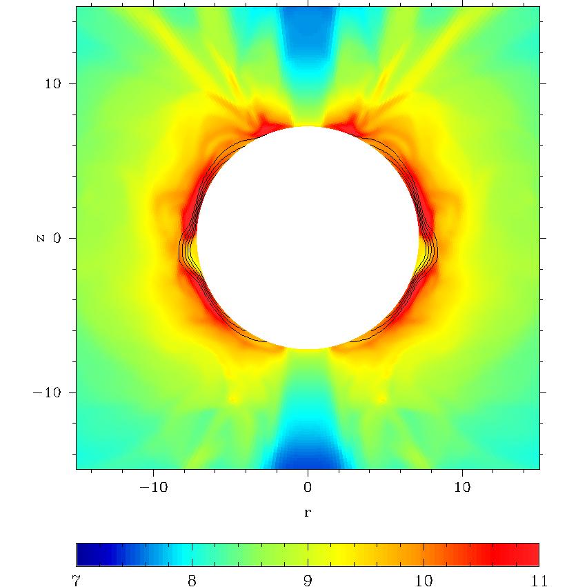
Figure 4: Model D at time $t=169$ms. The colour image shows $log_{10}\rho$ and the contours show the magnetic field lines. The unit length in all figures in this paper is ${\cal L}=GM/c^{2}\simeq 2$km.

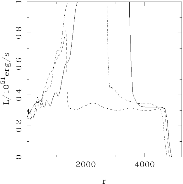
Figure 5: Total free energy flux through sphere of radius $r$ for model A (solid line), model B (dashed line), and model C (dash-dotted line).

Figure 2 shows the global structure of model B at the same time. The most apparent difference is in the size of the quasi-spherical supernova shock. It propagates noticeable slower because of the lower energy deposited in the radiation bubble. However, the propagation speed of the jets is almost the same as in model A suggesting that their power must be similar as well. One can also see that inside the supernova envelope the jets propagate inside a relatively thin channel and outside of the envelope they propagate through a low density cocoon inflated during the previous evolution. A similar cocoon is beginning to form in model A (see fig.1) suggesting that at later times models A and B could look even more alike.

Figure 3 shows the global structure of model C at time $t=277$ms. Since the ram pressure of the infalling material is higher than in models A and B the jet propagation speed is somewhat lower. The same factor explains lower propagation speed of the supernova shock in this model compared to model A. In other respects the solution is not much different.

The evolution of model D starts in very much the same fashion as for other models but at later times we observe a substantial fall-back of the shocked stellar material on the magnetar. The neutrino-cooled accreting matter eventually blocks the jet channel and squashes the magnetosphere against the star surface (see fig.4). Soon after the code crashes as the conditions near the surface become too extreme.

Figure 5 shows the total flux of “free energy”, the total energy at infinity minus the rest mass energy, as a function of radius for models A,B, and C. The “spikes” at $r\simeq 1000$ for model B, between $r=1000$ and $r=4000$ for model A, and between $r=1000$ and $r=3000$ for model C correspond to the blast wave of normal supernova explosion. The “plateaus” to the left and to the right of the spikes correspond to the jets. Thus, in all models the spin-down power released in the jets is indeed more or less the same, $L\simeq 3\times 10^{50}$erg/s. The corresponding spin-down time is $\simeq 37$s suggesting that most of the rotational energy will be released after the jets break out from the progenitor star. While this is a promising result for the magnetar model of GRBs it also suggests that only a modest fraction of the total rotational energy of the magnetar can be transferred to the supernova ejecta. In all three models the ratio of Poynting flux to the rest mass energy flux is $\sigma\simeq 2.5$. This is approximately 5 times higher than the value predicted by the theory of unconfined equatorial magnetar wind (see eq.(27) in Metzger et al.[Metzger et al. 2007]).

Figure 6 shows model A at the early times, $t\simeq 21$ ms. One can see that the magnetar is already producing an outflow which has blown a cavity in the shape of a column inside the collapsing star. The radius of this column is close to the radius of magnetar’s light cylinder, $R_{\mbox{\tiny LC}}\simeq 50MG/c^{2}=100$ km, which is shown in the right panel of fig.6 by the dashed line. We note, however, that for $z<100$ the column is still inside the light cylinder. The total pressure of the outflow is dominated by the magnetic field, the ratio of magnetic to gas pressure varying between 10 and 300. One can see strong axial compression of the outflow due to the hoop stress of azimuthal magnetic field. The distribution of total pressure over the boundary of the volume occupied by the outflow has a clear maximum at the point of intersection with the polar axis which is obviously related to the axial compression. This distribution explains the faster expansion of the cavity blown by the outflow in the axial direction. In the middle panel of fig.6 one can see the bow shock, at $z\simeq 600$, driven by the ouflow into the surrounding. There are no indications of the termination shock of the outflow itself - this is because the outflow is sub-fast. The solid line in the right panel of fig.6 shows the locus of points where the radial component of the phase velocity of ingoing Alfvén waves becomes positive. Inside the column these point form a closed surface which we call the Alfvén horizon of the magnetar-driven outflow. Any Alfvén wave can propagate from the exterior of this surface into its interior. One can see that the Alfvén horizon is always located inside the light cylinder, which agrees with theory of steady state MHD flows [Okamoto 1978].

Figure 7 shows the inner region of model A by the end of the run ($t\simeq 200$ ms). By this time the size of the central cavity, that develops a diamond-like shape, is significantly larger than $R_{\mbox{\tiny LC}}$, thanks to the decreased pressure in the surrounding bubble that resulted from its expansion in the course of supernova evolution. However, the rotational velocity in the equatorial plane is not ultra-relativistic indicating that the relativistic winding mechanism is not in operation. The velocity field (left and right panels of fig.7) shows that close to the magnetar the outflow is similar to an isotropic wind but then it becomes progressively collimated in the polar direction and eventually passes through the “bottle-neck” nozzles at the axial corners of the diamond. The collimation is smooth with no indication of shocks waves which is expected because the flow is always sub-fast.

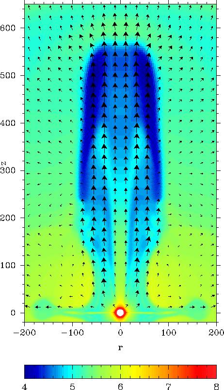
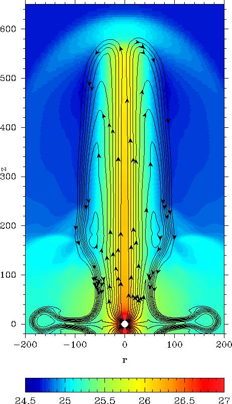
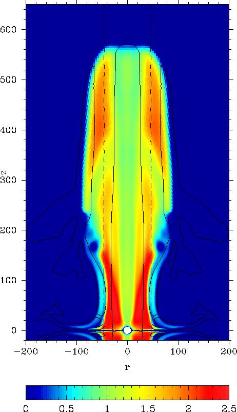
Figure 6: Model A at $t\simeq 21$ ms. Left panel: $\log_{10}\rho$ and the poloidal velocity field; Middle panel: The colour image shows $\log_{10}p_{\mbox{\tiny tot}}$, total pressure, and the contours show the magnetic flux function; Right panel: The colour image shows $\log_{10}(p_{\mbox{\tiny m}}/p_{\mbox{\tiny g}})$, the ratio of magnetic pressure to the gas pressure. The solid lines show the surfaces where the radial phase speed of ingoing Alfvén waves is zero - the one closest to the symmetry axis is the “Alfvén horizon”. The dashed line shows the location of the light cylinder.

After passing trough the nozzle each jet enters the channel made during the previous evolution and propagates inside a low density cocoon. In its outer layer the cocoon contains poloidal field lines of opposite direction to that of the jet and closer to the jet one can see magnetic islands and evidence of vortex motion. These islands are mostly remnants of plasmons injected from the dead zone of magnetar’s magnetosphere (see the right panel of fig.8) during its oscillatory cycle. In the middle panel of fig.7 one can see one of such recently ejected plasmons. Close inspection of animated pictures suggests the following origin of the oscillations. When the dead zone includes the highest magnetic flux it gradually accumulates plasma supplied from the magnetar surface. This leads to increase of the centrifugal force and expanding of the dead zone. Its magnetic field lines stretch in the equatorial direction trying to open up. The process seems to accelerate as the dead zone plasma moves further out from the star and finally escapes in eruptive manner leaving behind thin equatorial current sheet. Then the oppositely directed field lines of the sheet reconnect and this restores the initial configuration of the dead zone (a similar behavior of PNS magnetosphere was reported in Bucciantini et al., 2006). The amplitude of these oscillations is large so one gets the impression of the magnetosphere “breathing heavily”. Since here we integrate the equations of ideal RMHD it is the numerical resistivity that is responsible for the observed reconnection and the reliability of its time-scale is unclear.

The plots of fig.7 also reveal a rather peculiar time-dependent structure inside the diamond cavity and near to the polar axis, to which we will refer as the “trap zone”. It begins at $z\leq 50$ and continues almost up to the top corner of the cavity. In the right panel of fig.7, that shows the ration of magnetic to gas pressure (the inverse of the traditional magnetization parameter $\beta$), it looks as the region of lower magnetization. The density and velocity plots of fig.7 show that the trap zone has a relatively high density and low speed. In fact, the radial velocity in the trap zone changes sign both in space and time - the density clumps seen in the trap zone exhibit oscillatory motion along the polar axis. This explains the peculiar turns of magnetic field lines in the trap zone (see the middle panel of fig.7). From time to time plasma clouds are ejected from this zone and the time-scale of this ejections is similar to the time-scale of global magnetospheric oscillations. One of such clouds is seen in density plot of fig.7 at $z\simeq 650$. Another peculiarity of this zone, to which we have no explanation, is that it is separated from the polar axis by cylindrical shell, of radius $R\simeq R_{\mbox{\tiny LC}}$, with a relatively high velocity.

Figure 8 provides with additional information on the magnetic structure of this solution. One can see that the azimuthal magnetic field dominates almost everywhere in the “diamond zone” and in the jet, with the exception of the region immediately around the symmetry axis. $B^{\phi}/B_{p}$ is particularly high in the middle of the magnetic cocoon where the poloidal field changes direction (see the left panel of fig.8). However, the azimuthal field changes sign only in the equatorial current sheet. This is clearly seen in the middle panel of fig.8 which shows that $B^{\phi}$ does not vanish anywhere else. The electric current is concentrated in the jet core, the cocoon surface, and the equatorial current sheet thus showing that within most of the jet volume the magnetic field is almost force-free. The right panel of fig.8 shows the most inner part of the magnetar magnetosphere and reveals the existence of its dead zone.

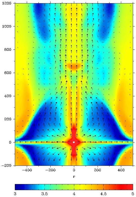
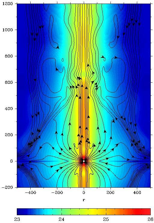
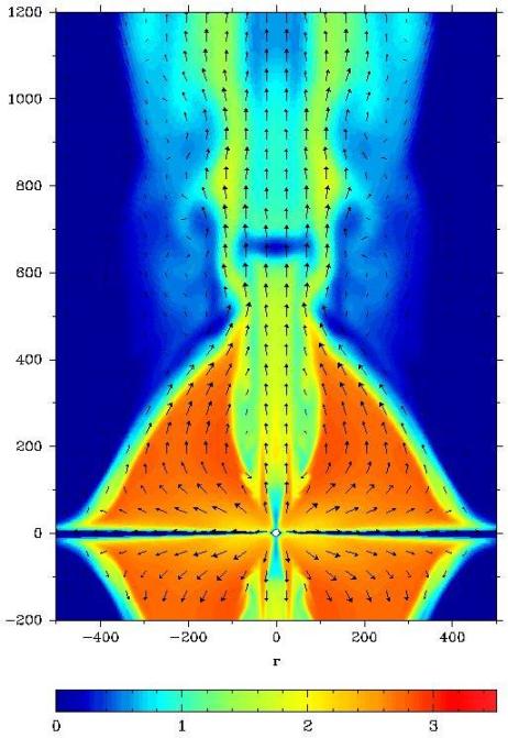
Figure 7: Model A at $t\simeq 200$ ms. Left panel: $\log_{10}\rho$ and the poloidal velocity field; Middle panel: The colour image shows $\log_{10}p_{\mbox{\tiny tot}}$, total pressure, and the contours show the magnetic flux function; Right panel: $\log_{10}(p_{\mbox{\tiny m}}/p_{\mbox{\tiny g}})$, the ratio of magnetic pressure to the gas pressure and the velocity field.

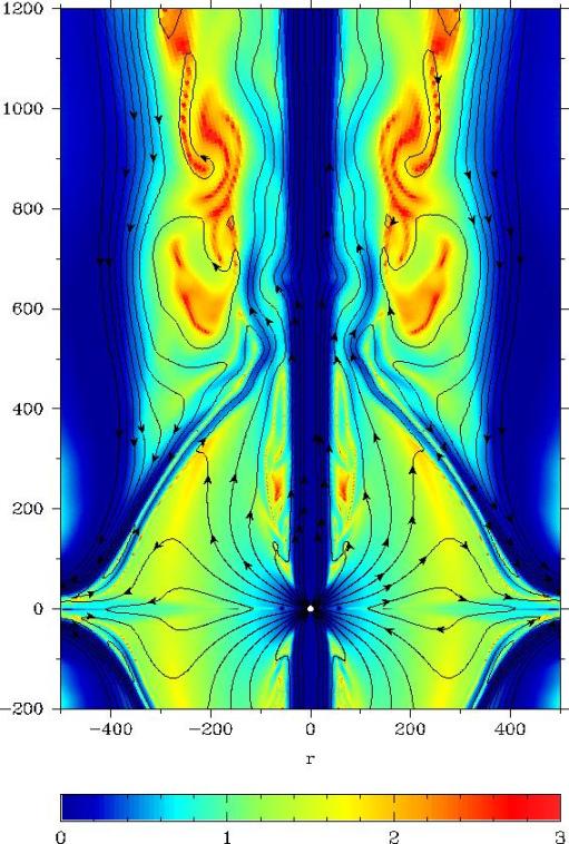
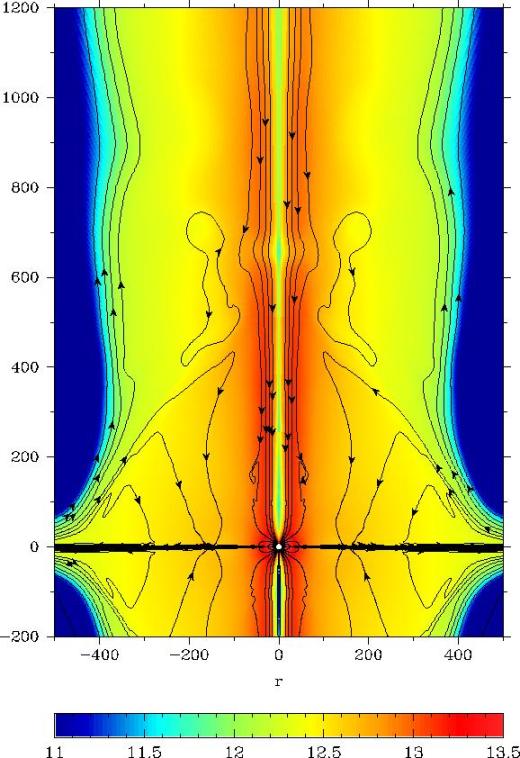
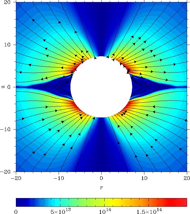
Figure 8: Model A at $t\simeq 200$ ms. Left panel: The colour image shows $\log_{10}(|B^{\phi}|/B_{pol})$, the ratio of azimuthal and poloidal components of magnetic field, and the contours show the lines of poloidal magnetic field; Middle panel: The colour image shows the magnitude of the azimuthal magnetic field, $\log_{10}|B^{\phi}|$, and the contours show the lines of electric current. Right panel: The colour image shows the amplitude of $B^{\phi}$ and the contours show the lines of poloidal magnetic field. The unit length in all figures in this paper is ${\cal L}=GM/c^{2}\simeq 2$km.

4 Discussion

4.1 Cautionary notes

The main motivation of this study was to explore the effects that the birth of a millisecond magnetar may have on the development of delayed supernova explosions. The problem of supernova explosions is extremely complicated and we had to make a number of simplifying assumptions driven by the limitations of our numerical method. The most problematic issue is the initial setup where we assume that the magnetic field of the magnetar generated via $\alpha$-$\Omega$-dynamo or other dynamo has just emerged above magnetar’s surface and the large amount of energy needed to drive standard supernova explosion have just been deposited in the radiation bubble. Although the time-scales of these processes are similar ($\leq 1s$), even small asynchronism can significantly change the initial conditions simply because of the large expansion speed of the supernova shock. This has to be kept in mind when analyzing our numerical models, particularly their early evolution. However, we expect the models to be more or less reliable in the second half of the simulation runs.

Another important limitation of our models, as well as many other models of magnetically-driven astrophysical flows, concerns the potentially destructive role of the kink mode instabilities. Obviously, these instabilities are totally suppressed in our axisymmetric simulations and full 3D simulations are needed to investigate this issue. We can only comment on two stabilizing factors present in the current setting. Close to the magnetar the poloidal magnetic field may provide strong “backbone” support for the outflows [Anderson et al. 2006]. Further away the jets propagate within a channel with “high-inertia walls” which could effectively dump the kink-type motions inside the channel.

Finally, the condition of axisymmetry means that we can only study the exceptional case of aligned rotator. However, we do not expect the case of oblique rotator to give dramatically different results. For example, in the limit of Magnetodynamics (inertia-free Relativistic MHD) the spin-down power of orthogonal rotator exceeds that of aligned rotator but only by a factor of two [Spitkovsky 2006]

4.2 Comments on the mechanism of explosion

Many features of the magnetar driven outflows observed in our simulations are similar to those predicted by Uzdensky & McFadyen [Uzdensky & MacFadyen 2006]. There is however a number of important differences and one of them is the nature of explosion. None of the succesful explosions in our simulations are magnetically driven. These explosions are produced via the deposition of thermal energy in the radiation bubble of the initial solution. We have never seen the long phase (many rotational periods) of building up of magnetic pressure behind the stalled shock – the key process in their scenario. Moreover, in the simulation runs where the amount of energy deposited in the buble was reduced in order to approach the conditions of failed supernova and to engage the magnetic mechanism the magnetar magnetosphere did not expand but was pressed back to the magnetar surface under the weight of neutrino-cooled layers of accreting material. It is easy to see why. Suppose that mass $\Delta M$ passes through the stalled shock of failed supernova and accumulates at the radius of the light cylinder $r_{\mbox{\tiny LC}}=100$km (the critical radius in the magnetic mechanism). Then its weight will be $N=GM\Delta M/4\pi r^{4}_{\mbox{\tiny LC}}\simeq 3\times 10^{28}\mbox{g}\,\mbox{cm}^{-1}\mbox{s}^{-2}$ for the relatively small $\Delta M=0.01M_{\sun}$. This is much larger than the pressure of the dipolar magnetic field at the same radius, $P_{m}\simeq 1.3\times 10^{26}\mbox{g}\,\mbox{cm}^{-1}\mbox{s}^{-2}$ (for this estimate we assume that the at the PNS surface $B_{0}=10^{15}$G). Similarly, one finds that the ram pressure of the free-falling stellar material at the light cylinder is also much larger than the magnetic pressure. In principle, the magnetic field generated in the PNS can be transported in the region bounded by the stalled shock of failed supernova by the large scale convective motions developing in this region and even to be locally amplified via some sort of dynamo. However, in this case the dynamics of magnetic field would be much more complicated than the one described in the simple magnetospheric model of Uzdensky & McFadyen [Uzdensky & MacFadyen 2006] and in order to capture it one would require much more sophysticated simulations than ours.

4.3 Magnetised winds and magnetic towers

Until recently the magnetically driven outflows from astrophysical objects were classified only as “winds” or “jets”, depending on whether the outflow proceeds in all directions or it is collimated within a cone due external confinement of one sort or another. But since the work of Lynden-Bell[Lynden-Bell 1996, Lynden-Bell 2003], who proposed a particular magnetic mechanism for generation of astrophysical gets, a new term, “magnetic tower” is gradually gaining popularity too. In many computer simulations the development of column-like outflows have been observed and these outflows have been pronounced magnetic towers, without a detailed analysis. In fact, collimated winds and magnetic towers have many similar properties like the magnetic braking of the central rotator, the amplification of azimuthal magnetic field, the axial compression due to hoop stress etc. A magnetic tower occupies a finite volume which gradually increases in time whereas winds are usually associated with steady-state solutions that extend to infinity. However, once a wind becomes super-fast its interaction with the external medium does not affect the upstream solution and thus this distinction is superficial. A magnetic tower is prevented from lateral expansion by external pressure but some kind of external force is needed to confine any type of magnetic flow within a finite volume. The magnetic field lines of magnetic tower have both foot-point anchored to the rotator but the same can be said about the wind from a star with, for example, a dipolar magnetic field; the so-called open magnetic field lines of stellar winds close far in the wind zone.

From our view the main distinction between a magnetic tower and a magnetically driven wind is in the way the azimuthal magnetic field is generated in these flows. In the magnetic tower model the azimuthal field is generated solely due the differential rotation at its base (originally an accretion disk) which causes winding of closed magnetic field lines whose foot points rotate with different angular velocities. Thus, both these foot points are assumed to be in communication with each other by means of torsional Alfvén waves; the faster rotating foot-point creates stronger wave and wins in the sense that its rotation determines the sigh of the generated azimuthal field. This also implies that the magnetic tower is a quasi-magnetostatic configuration - the vertical growth of the tower can be considered as a sequence of magnetostatic models parametrized by time.

In contrast, wind solutions are characterized by the appearance of Alfvén horizon; once the Alfvén waves emitted by the rotator cross this surface they can no longer come back. Then the closed field lines of rotator’s magnetic field may form two groups: (1) those that close within the horizon and (2) those that close outside of it. If a magnetic field line belongs to the first group then its foot points can communicate by means of Alfvén waves. In this case it is still important whether the rotation at the base is differential or not. If, however, it belongs to the second group then the communication is broken and for this reason the field line can cosidered as opened. For example, the magnetosphere of a solidly rotating star with dipolar magnetic field has two zones: the so-called “dead zone” where the magnetospheric plasma corotates with the star and the magnetic field is purely poloidal, and the “wind zone” where the magnetic field lines are “opened” and the magnetic field has an azimuthal component. The magnitude of this component depends on the angular velocity of only one foot point, the upstream one, and it is created solely by the Alfvén waves emitted from this point. One may say that the winding of magnetic field in the wind zone is the feedback reaction of plasma on the magnetic field that tries to spin it up, it is there due to the finite inertia uploaded on the magnetic field lines in the wind. There is also finite inertia in the dead zone but in the absence of outflow there is also plenty of time to enforce full corotation.

Formally, the magnetic tower solutions can be constructed for a rather arbitrary distributions of external pressure [Lynden-Bell 2003]. However, for real flows with finite Alfvén speed the lateral expansion due to declining external pressure can be a factor that works in favor of wind solutions. Indeed, the non-relativistic Alfvén speed $v_{a}\propto B_{p}/\sqrt{\rho}$. If $\varpi$ is the cylindrical radius of a magnetic surface then to zero-order approximation we have $B_{p}\propto\varpi^{-2}$ and, assuming constant mass loading of magnetic field lines, $\rho\propto\varpi^{-2}$. This gives $v_{a}\propto\varpi^{-1}$ and if the speed of longitudinal expansion does not decrease as fast as this then at some point the outflow will become super-Alfvenic. This would signify a transition to the wind regime.

Relativity further complicates the matter as it puts an upper limit on the location of Alfvén surface - it must reside inside the light cylinder [Okamoto 1978]. This seems to be related to the fact that in relativistic MHD there is inertial mass associated with the magnetic (or rather electromagnetic) field itself. In fact, in the limit of Magnetodynamics, that is relativistic MHD with vanishingly small particle inertia (e.g. Komissarov 2002, Komissarov et al.2007), all of the inertia is due to electromagnetic field and these surfaces coincide – this is why the light cylinder plays such an important role in the theory of pulsar winds. In this respect we wish to comment on the “pulsar-in-cavity” problem of Uzdensky and MacFadyen[Uzdensky & MacFadyen 2006]. They consider a magnetized neutron star placed in the center of an empty cavity inside a collapsing supernova progenitor. The radius of this cavity is assumed to exceed the radius of star’s light cylinder. By making the cavity so large they effectively create conditions that allow the development of a pulsar wind with the kind of magnetic winding that is specific only to winds (notice that the star rotates as a solid body). Rather unfortunately, however, they still call the outflow that may eventually develope in this problem a magnetic tower.

Summarizing, we wish to stress that both in analytical and numerical modeling of magnetically driven ouflows it is very important to determine whether the Alfven horizon appears or not. When the magnetic tower approximation is used this gives a key test of its validity. When the results of computer simulations are analysed this helps to understand the physical nature of the outflow.

4.4 The nature of magnetar-driven jets

As the thermally driven explosion (caused by the energy deposition in the radiation bubble) develops in our simulations a rarefaction is created in the center and the magnetar magnetosphere begins to expand, predominantly in the equatorial direction. During this initial expansion an Alfvén horizon appears inside the magnetosphere and a magnetar wind begins to develop which injects azimuthal magnetic flux and energy into the surrounding space. Because the expansion is slow compared to the fast magnetosonic speed the fast waves quickly establish approximate magnetostatic equilibrium inside the “magnetic cavity” and the hoop stress of the azimuthal magnetic field ensures that this equilibrium is characterised by an axial compression. As a result the normal stress on the cavity surface develops a maximum at the poles, the cavity begins to expand predominantly in the polar direction and the polar jets are beginning to form (see fig.6). The jets remain sub-fast up to the very end of the simulations and the termination shock never develops. However, the jet total pressure is sufficiently high to drive bow shocks into the surrounding. In fact the structure of ouflow is quite similar to that anticipated in Uzdensky and MacFadyen[Uzdensky & MacFadyen 2006]. There are however some qualitative differences. First of all, the jets develop before the cavity expands beyond the light cylinder. This is not very suprizing because the wind magnetization is not ultrarelativistic and the Alfvén surface can be well inside the light cylinder. Secondly, there is no highly relativistic plasma rotation in the equatorial plane, even when the cavity expands well beyond the light cylinder.

Eventually, as the central cavity becomes sufficiently large, one would expect the magnetar wind to become super-fast and the wind termination shock to appear, as it is assumed in [Bucciantini et al. 2007a, Bucciantini et al. 2007b]. However, additional studies are required to determine when exactly this will occur. This issue may be further complicated by the magnetar cooling which leads to higher magnetization of the wind and moves its fast surface further away . In any case our results suggest that by the time of transition to super-fast regime the magnetar-driven jets will already be well established and thus the initial setup used in [Bucciantini et al. 2007a, Bucciantini et al. 2007b], where the central cavity is assumed to be large and spherical, may be somewhat unrealistic.

4.5 Magnetar as a cenral engine of GRB jets

Our results show that magnetically-driven outflows from millisecond magnetars can become highly anisotropic jets at the very early stages of supernova explosions. Assuming that their propagation speed does not decrease in time, these jets would traverse the progenitor star of radius $\simeq 2\times 10^{10}$cm in about 4 seconds. After this the spin-down energy of PNS will be carried away by the jets into the surrounding space and the rate of energy transfer to the supernova ejecta will drop. The total power of long duration GRB-jets is not well known but the observations of radio afterglows which are no longer subject of relativistic beaming suggest that it can be high, $\simeq 5\times 10^{51}$erg [Berger et al. 2004], well in agreement with our results. Since the combined total power of both jets in our simulations is $\simeq 3\times 10^{50}\mbox{erg}/\mbox{s}$, prior to the break out the energy transferred to the supernova ejecta will be only $\leq 10^{51}\mbox{erg}$, noticeably less than what is usually derived for hypernovae. Thus, on one hand our results provide the first self-consistent numerical model of a central engine capable of producing, on a long-term basis, collimated jets with sufficient energy to explain GRBs and their afterglows. On the other hand, the relatively small amount of energy transferred the supernova ejecta could be a problem due to the connection between high velocity SNe and long GRBs. Although the connection between SNe and GRBs is supported by strong circumstantial evidence, the direct evidence is still scarce with only handful of SNe identified with GRBs. It is quite possible that the current paradigm connecting GRBs with HNe is simply a reflection of the observational bias towards more powerful events [Woosley & Bloom 2006, Della Valle 2006]. SN 2002LT/GRB 021211 may the case of a GRB produced by a standard SN Ib/c [Della Valle 2006].

The relatively high propagation speed of jets in our simulations may in part be attributed to the condition of axisymmetry. The hydro-simulations of 2D slab jets (e.g. Komissarov & Falle 2003) and 3D round jets [Norman 1996] show significantly lower propagation speeds of jets without enforced mirror or axial symmetry as the kink modes of current-driven or pressure-driven instabilities result in redistribution of the pressure force over larger area at the jet head (cf. Aloy et al.,1999). On the other hand, as the jets enter progressively less dense outer layers of collapsing star their propagation speed may actually increase. Slower propagation speed would increase the amount of energy transferred to the supernova ejecta and reduce the energy available to produce GRB.

Although our jets are not as fast as required by the observations of GRBs the gradual cooling of PNS would lead to lower mass loading and hence higher terminal speed of the jets later on. Indeed, according to the computations of Pons et al.[Pons et al. 1999] the neutrino luminosity of PNS decreases by a factor of 10 already during the first 10s and then enters the phase of rapid exponential decline, largely independent on the details of initial models and EOS. Metzger et al.[Metzger et al. 2007] argue that the magnetization $\sigma=100-1000$ can be reached when the the PNS still has enough rotational energy to power a GRB. This corresponds to the asymptotic Lorentz factor in the range of $\Gamma_{\infty}=\sigma/2=50-500$ (e.g. Vlahakis 2004). However, the magnetic acceleration of relativistic flows is a rather slow process and we do not expect the termination speeds to be reached within the stellar boundaries. Further studies are needed to clarify the issue of magnetic acceleration.

Since the cooling time of PNS is comparable with the break out time, and the time-scale of long duration GRBs, one would expect that that at the time of break out the mass-loading of the PNS magnetosphere will still be quite high and thus the flow speed of the jets will still be relatively low, $\Gamma\simeq 1-10$. Only later the Lorentz factor will gradually increase and eventually reach the ultra-relativistic values, $\Gamma\simeq 200$, inferred for the GRB jets. The implications of such a non-uniform jet structure, with Lorentz factor gradually decreasing with distance from the the star, for both the prompt and the afterglow emission of GRBs remain to be investigated. Here we point out only few obvious points. First of all one may expect some similarities with the model of structured jet [Mészáros et al. 1998, Dai & Gou 2001, Panaitescu 2005, Rossi et al. 2002, Wei & Jin 2003, Kumar & Granot 2003], whose Lorentz factor varies with polar angle, and the model of two-component jet [Mészáros & Rees 2001, Vlahakis et.al. 2003, Zhang et al. 2003, Ramirez-Ruiz et al. 2002, Mizuta et al. 2006, Granot et al. 2006, Jin et al. 2006, Morsony et al. 2006, Willingale et al. 2007]. Secondly, since lower Lorentz factor results in weaker Doppler effect one would expect softer emission from the parts of the jet emitted earlier and located further away from the star. This could be the origin of the prompt optical and X-ray emission and early afterglows. Curiously enough, the model suggests that the zero-point of gamma-ray bursts lags behind the zero points of prompt X-ray and optical bursts. Finally, while the collision between the slower earlier jet and the ISM or the progenitor wind would still produce the strong forward shock usually associated with afterglows, one might expect a secondary strong forward shock where the faster late jet collides with the slower early jet. This secondary shock will propagate faster than the primary one and will eventually catch up with it. Its emission, which will be harder and beamed more strongly than that of the primary shock, may lead to distinctive features in the light curves of afterglows.

It is tempting to consider the global oscillation of magnetar’s magnetosphere and the related non-stationary plasma ejection as the origin of “inner shocks” invoked in models of prompt GRB emission [Piran 2005b]. However, it is important to check if the reconnection rate is determined mainly by the global dynamics and not by the resistivity model (which was purely numerical in our simulations). Moreover, it remains to be seen if such oscillations can persist at later times ($t>$ few seconds) when the the mass-loading of the magnetosphere drops and the inner “cavity” significantly increases in size. Later, when the jet becomes super-fast, internal shocks can be produced via interaction with inhomogeneous time-dependent cocoon and instabilities. The inhomogeneous structure of the slow jet may also lead to variable emission from the secondary forward shock.

5 Conclusions

The results of our study show that when a core collapse of a massive star results in a birth of a millisecond proto neutron star with super-strong magnetic field (proto-magnetar), this could have a spectacular effect on the supernova explosion. During the very early stage of the explosion the magnetar can produce highly collimated jets capable of puncturing the collapsing star in a matter of seconds. The spin-down time of the proto-magnetar is an order of magnitude longer thus suggesting that a large fraction of its rotational energy, $E\simeq 10^{52}$erg, will be carried by the jets into the surrounding space. This supports the idea that at least some long duration Gamma Ray Bursts can have millisecond magnetars as their central engines.

The magnetic outflow is best described as a sub-fast super-Alfvénic collimated wind. The super-Alfvénic nature of the flow explains the generation of azimuthal magnetic field which soon begins to dominate the flow dynamics. The collimation is a combined effect of the inertial confinement by the stellar material and the hoop stress of the azimuthal field. The outflow is not a magnetic tower.

It remains to be seen as to how soon the wind in the central cavity becomes super-fast and a proto-PWN is formed inside the collapsing star. The magnetic acceleration of the jets inside the channels bored through the star and outside of the star is also an important subject for future study.

It is very likely that the GRB jets produced in this fashion first emerge as only moderately relativistic flows and only later as the magnetar cools they become ultra-relativistic. The effect of this on both the prompt and the early afterglow emission needs further investigation

A non-magnetic, e.g. the delayed neutrino-driven explosion of power comparable to that of normal core-collapse supernovae is needed to turn-on the magnetic mechanism. Otherwise the PNS magnetosphere is unable to expand end develop a super-Alfvénic wind. The idea that a failed supernova explosion can be revived by a millisecond magnetar does not seem to work.

References

- [Akiyama et al. 2003] Akiyama S., Wheeler J.C., Meier D.L., Lichtenstadt I., 2003, ApJ, 584, 954
- [Akiyama & Wheeler 2005] Akiyama S., Wheeler J.C., 2005, ApJ, 629, 414
- [Aloy et al. 1999] Aloy M.A., Ibanez J.M., Marti J.M., Gomez J.-L., Muller E., 1999, ApJ, 523, L125
- [Anderson et al. 2006] Anderson J.M., Li Z.-Y., Krasnopolsky R., Blandford R.D., 2006, ApJ, 653, L33
- [Ardeljan et al. 2005] Ardeljan N.V., Bisnovatyi-Kogan G.S., Moiseenko S.G., 2005, MNRAS, 359, 333
- [Balbus & Hawley 1991] Balbus S.A., Hawley J.F., 1991, ApJ, 376, 214
- [Begelman 1992] Begelman M.C., Li Z.-Y., 1992, ApJ, 397, 187
- [Berger et al. 2004] Berger E., Kulkarni S.R., Frail D.A., 2004, ApJ, 612, 966
- [Bethe 1990] Bethe H.A., 1990, Rev.Mod.Phys., 62, 801
- [Bisnovatyi-Kogan 1970] Bisnovatyi-Kogan G.S., 1970, Astron.Zh., 47, 813 (Soviet Astron., 1971, 14, 652)
- [Bisnovatyi-Kogan 1976] Bisnovatyi-Kogan G.S., Popov Yu.P., Samokhin A.A., 1976, ApSS, 41, 321
- [Blondin et al. 2003] Blondin J.M., Mezzacappa A., DeMario C., 2003, ApJ, 584, 971
- [Bucciantini et al. 2006] Bucciantini N., Thompson T.A., Arons J., Quataert E., Del Zanna L., 2006, MNRAS, 368, 1717
- [Bucciantini et al. 2007a] Bucciantini N., Quataert E., Arons J., Metzger B.B., Thompson T.A., 2007a, arXiv:0705.1742
- [Bucciantini et al. 2007b] Bucciantini N., Quataert E., Arons J., Metzger B.B., Thompson T.A., 2007b, arXiv0707.2100
- [Burrows & Lattimer 1986] Burrows A., Lattimer J.M., 1986, ApJ, 307, 178
- [Burrows et al. 2006] Burrows A., Livne E., Dessart L., Livne E., Ott C.D., Murphy J., 2006, ApJ, 640, 878
- [Burrows et al. 2007] Burrows A., Dessart L., Livne E., Ott C.D., Murphy J., 2007, ApJ, 664, 416 (astro-ph/0702539)
- [Cardall & Fuller 1997] Cardall C.Y., Fuller G.M., 1997, ApJ, 486, L111
- [Dai & Gou 2001] Dai Z.G., Gou L.J., 2001, ApJ, 552, 72
- [Di Matteo et al. 2002] Di Matteo T., Perna R., Narayan R., 2002, ApJ., 576, 706
- [Della Valle 2006] Della Valle M., 2006, Chin.J.Astron.Astrophys., v6, Suppl.1, 315
- [Duncan & Thompson 1992] Duncan R.C., Thompson T.A., 1992, ApJ, 392, L9
- [Granot et al. 2006] Granot J., Konigl A., Piran T., 2006, MNRAS, 370, 1946
- [Ivanova et al. 1969] Ivanova L.N., Imshennik V.S., Nadezhin D.K., 1969, Sci.Inf.Astr.Council.Acad.Sci, 13,3
- [Jin et al. 2006] Jin Z.P., Yan T., Fan Y.Z., Wei D.M., 2007, ApJ, 656, L57
- [Khokhlov et al. 1999] Khokhlov A.M., Hoflich P.A., Oran E.S., Wheeler J.C., Wang L., Chtchelkanova A.Yu., 1999, ApJ, 524, L107
- [Komissarov 1999] Komissarov S.S., 1999, MNRAS, 303, 343
- [Komissarov & Falle 2003] Komissarov S.S., Falle S.A.E.G, 2003, MNRAS, 343, 1045
- [Komissarov 2002] Komissarov S.S., 2002, MNRAS, 336, 759
- [Komissarov 2004a] Komissarov S.S., 2004a, MNRAS, 350, 427
- [Komissarov 2004b] Komissarov S.S., 2004b, MNRAS, 350, 1431
- [Komissarov 2006] Komissarov S.S., 2006, MNRAS, 368, 993
- [Komissarov et al. 2007a] Komissarov S.S., Barkov M., Lyutikov M., 2007a, MNRAS, 374, 415.
- [Komissarov et al. 2007b] Komissarov S.S., Barkov M.V., Vlahakis N., Königl A., 2007b, MNRAS, online early.
- [Kotake et al. 2004] Kotake K., Sawai H., Yamada S., Sato K., 2004, ApJ, 608, 391
- [Kumar & Granot 2003] Kumar P., Granot J., 2003, ApJ, 591, 1086
- [LeBlanc & Wilson 1970] LeBlanc L.M., Wilson J.R., 1970, ApJ, 161, 541
- [Lynden-Bell 1996] Lynden-Bell D., 1996, MNRAS, 279, 389
- [Lynden-Bell 2003] Lynden-Bell D., 2003, MNRAS, 341, 1360
- [Lyutikov & Blandford 2003] Lyutikov M., Blandford R.D., 2003, astro-ph/0312347
- [MacFadyen & Woosley 1999] MacFadyen A.I. & Woosley S.E, 1999, ApJ,524, 262
- [Masada et al. 2007] Masada Y., Sato T., Shibata K., 2007, ApJ, 655, 447
- [Mészáros et al. 1998] Mészáros P., Rees M.J., Wijers R.A.M.J., 1998, ApJ, 499, 301
- [Mészáros & Rees 2001] Mészáros P., Rees M.J., 2001, ApJ, 556, L37
- [Metzger et al. 2007] Metzger B.D., Thompson T.A., & Quataert E., 2007, ApJ, 659, 561
- [Meier et al. 1976] Meier D.L., Epstein R.E., Arnett W.D., Schramm D.N., 1976 ,ApJ, 204, 869
- [Mizuno et al. 2004] Mizuno Y., Yamada S., Koide S., Shibata K., 2004, ApJ, 606, 395
- [Mizuta et al. 2006] Mizuta A., Yamasaki T., Nagataki S., Mineshige S., 2006, ApJ, 651, 960
- [Moiseenko et al. 2006] Moiseenko S.G., Bisnovatyi-Kogan G.S., Ardeljan N.V., 2006, MNRAS, 370, 501
- [Morsony et al. 2006] Morsony b.j., lazzati d., begelman m.c., 2006, astro-ph/0609262
- [Nagataki et al. 2007] Nagataki S., Takahashi R., Mizuta A., Takiwaki T., 2007, ApJ, 659, 512
- [Narayan et al. 2001] Narayan R., Piran T., Kumar P., 2001, ApJ, 557, 949
- [Nomoto et al. 2004] Nomoto K. et al., 2004, in Stellar Collapse, ed. C.Fryer,Kluwer,Dordrecht, p277
- [Norman 1996] Norman M.,1996, in Energy transport in radio galaxies and quasars, Proceedings of a workshop held in Tuscaloosa, Alabama, 19-23 Sep 1995, eds Hardee P.E., Bridle A.H., Zensus J.A., ASP Conference Series, SanFrancisco v.100, p.319
- [Obergaulinger 2006] Obergaulinger M., Aloy M.A., Dimmelmeier H., & Muller E., 2006, A&A, 457, 209
- [Okamoto 1978] Okamoto I., 1978, MNRAS, 185, 69O
- [Panaitescu 2005] Panaitescu A., 2005, MNRAS, 363, 1409
- [Panaitescu 2006] Panaitescu A., 2005, astro-ph/0612170
- [Piran 2005a] Piran T., 2005a, Rev.Mod.Phys., 76, 1143
- [Piran 2005b] Piran T., 2005b, Nuovo Cim. 28C, 373
- [Pons et al. 1999] Pons J.A., Reddy S., Prakash M., Lattimer J.M., Miralles J.A., 1999, ApJ, 513, 780
- [Proga et al. 2003] Proga D., MacFadyen A.I., Armitage P.J., Begelman M.C., 2003, ApJ, 599, L5
- [Proga 2005] Proga D., 2005, ApJ, 629, 397
- [Ramirez-Ruiz et al. 2002] Ramirez-Ruiz E., Celotti A., Rees M.J., 2002, MNRAS, 337, 1349
- [Rossi et al. 2002] Rossi E., Lazzati D., Rees M.J., 2002, MNRAS, 332, 945
- [Ruffert & Janka 1999] Ruffert M., Janka H.T., 1999, A&A, 344, 573
- [Salmonson & Wilson 1999] Salmonson J.D., Wilson J.R., 1999, ApJ, 517, 895
- [Schinder et al. 1987] Schinder P.J., Schramm D.N., Wiita P.J., Margolis S.H., Tubbs D.L., 1987, ApJ, 313, 531.
- [Shibata et al. 2006] Shibata M., Liu Y.T., Shapiro S.L., Stephens B.C., 2006, Phys.Rev D, 74, 104026,
- [Spitkovsky 2006] Spitkovsky A., 2006, ApJ Lett., 648, L51
- [Symbalisty 1984] Symbalisty E.M.D., 1984, ApJ, 285, 729
- [Takiwaki et al. 2004] Takiwaki T., Kotake K., Nagataki S., Sato K., 2004, ApJ, 616, 1086
- [Timmes & Swesty 2000] Timmes F.X., Swesty F.D., 2000, ApJSS, 126, 501
- [Thompson 2006] Thompson T.A.,2006, astro-ph/0611368
- [Thompson et al. 2001] Thompson T.A., Burrows A., Meyer B.S., 2001, ApJ, 562, 887
- [Thompson & Duncan 1993] Thompson C., Duncan R.C., 1993, ApJ, 408, 194
- [Thompson 1994] Thompson C., 1994, MNRAS, 270, 480
- [Thompson & Duncan 1995] Thompson C.,Duncan R.C., 1995, MNRAS, 275, 255
- [Thompson et al. 2004] Thompson T.A., Chang P., Quataert E., 2004, ApJ, 611, 380
- [Usov 1992] Usov V., 1992, Nature, 357, 472
- [Uzdensky & MacFadyen 2006] Uzdensky D.A. & MacFadyen A.I., 2006, astro-ph/0609047
- [Vlahakis 2004] Vlahakis N., 2004, Ap&SS, 293, 67
- [Vlahakis et.al. 2003] Vlahakis N., Peng F., Konigl A., 2003, ApJ, 594, L23
- [Vlahakis & Konigl 2003] Vlahakis N., Konigl A., 2003, ApJ, 596, 1080
- [Wang et al. 2002] Wang et al., 2002, ApJ, 579, 671
- [Wang et al. 2003] Wang L., Baade D., Höflich P., Wheeler J.C., 2003, ApJ,592, 457
- [Weber & Davis 1967] Weber E.J., Davis L.J., 1967, ApJ, 148, 217
- [Wei & Jin 2003] Wei D.M., Jin Z.P., 2003, A&A, 381, 731
- [Wheeler et al. 2000] Wheeler J.G., Yi I., Hoflich P., Wang L., 2000, ApJ, 537, 810
- [Wheeler et al. 2002] Wheeler J.G., Meier D.L., Wilson J.R., 2002, ApJ, 568, 807
- [Willingale et al. 2007] Willingale R. et al., 2007, ApJ, 662, 1093
- [Woods & Thompson 2004] Woods P.M. & Thompson C., 2004, in Compact Stellar X-ray Sources. ed. W.H.G.Lewin & M. van der Klis, Cambridge Univ. Press, Cambridge, p.547
- [Woosley & Baron 1992] Woosley S.E., Baron E., 1992, ApJ, 391, 228
- [Woosley & Bloom 2006] Woosley S.E., Bloom J.S., 2006, Ann.Rev.Astr.Astrophys., 44, 507
- [Yamada & Sawai 2004] Yamada S., Sawai H., 2004, ApJ, 608, 907
- [Zhang et al. 2003] Zhang W., Woosley S.E., MacFadyen A.I., 2003, ApJ, 586, 356