First detection of galaxy-galaxy-galaxy lensing in RCS

Abstract

Context. The weak gravitational lensing effect, small coherent distortions of galaxy images by means of a gravitational tidal field, can be used to study the relation between the matter and galaxy distribution.

Aims. In this context, weak lensing has so far only been used for considering a second-order correlation function that relates the matter density and galaxy number density as a function of separation. We implement two new, third-order correlation functions that have recently been suggested in the literature, and apply them to the Red-Sequence Cluster Survey. As a step towards exploiting these new correlators in the future, we demonstrate that it is possible, even with already existing data, to make significant measurements of third-order lensing correlations.

Methods. We develop an optimised computer code for the correlation functions. To test its reliability a set of tests involving mock shear catalogues are performed. The correlation functions are transformed to aperture statistics, which allow easy tests for remaining systematics in the data. In order to further verify the robustness of our measurement, the signal is shown to vanish when randomising the source ellipticities. Finally, the lensing signal is compared to crude predictions based on the halo-model.

Results. On angular scales between $\sim 1^{\prime}$ and $\sim 11^{\prime}$ a significant third-order correlation between two lens positions and one source ellipticity is found. We discuss this correlation function as a novel tool to study the average matter environment of pairs of galaxies. Correlating two source ellipticities and one lens position yields a less significant but nevertheless detectable signal on a scale of $\sim 4^{\prime}$. Both signals lie roughly within the range expected by theory which supports their cosmological origin.

1 Introduction

The continuous deflection of light rays propagating through the Universe by inhomogeneities of the large-scale distribution of matter generates a coherent, weak distortion pattern over the sky: the shear field. As the source of the shear field is gravity, the total matter distribution contributes to this effect. It is, therefore, a probe of the full matter content of the Universe. The shear field can be investigated by correlating the shapes of distant faint galaxies (e.g. Schneider 2006; Van Waerbeke & Mellier 2003; Bartelmann & Schneider 2001). Since the first detection of this effect (Bacon et al. 2000; Kaiser et al. 2000; Van Waerbeke et al. 2000; Wittman et al. 2000) studying the weak gravitational lensing effect has become an important tool for cosmology. Together with the next-generation weak lensing surveys such as the RCS2 (ongoing), CFHTLS (ongoing), Pan-STARRS 1 (commencing soon) or KIDS (planned to commence during the second half of 2008), the weak lensing effect will allow us to put tight constraints on cosmological parameters (Peacock et al. 2006).

One important topic in contemporary cosmology is the relation between the dark matter and the galaxy population, the latter of which is thought to form under particular conditions from the baryonic component within the dark matter density field. This relation can be studied by cross-correlating the shear signal and (angular) positions of a selected galaxy population.

As the shear is quite a noisy observable, higher order galaxy-shear correlation functions are increasingly difficult to measure. For this reason, studies in the past have focused on $2^{\rm nd}$-order statistics (“galaxy-galaxy lensing”, GGL hereafter) which involve one galaxy of the selected population (foreground) and one source galaxy (background) whose ellipticity carries the lensing signal. The GGL-signal can be used to learn more about the typical dark matter environment of single galaxies (most recently Kleinheinrich et al. 2006; Mandelbaum et al. 2006b, a, c; Seljak et al. 2005; Hoekstra et al. 2005, 2004; Sheldon et al. 2004), or the so-called galaxy biasing (Simon et al. 2007; Pen et al. 2003; Hoekstra et al. 2002a, 2001).

Schneider & Watts (2005) introduced “galaxy-galaxy-galaxy lensing” (GGGL) correlation functions and estimators thereof which allow us to move to the next, $3^{\rm rd}$-order level (see also Watts & Schneider 2005). The correlation functions now involve either two foreground galaxies and one background galaxy, or one foreground galaxy and two background galaxies. This idea was also discussed by Johnston (2006) who studied how to derive the galaxy-galaxy-mass correlation function, which is one of the foregoing two, from weak gravitational lensing. These functions, although more difficult to measure than the two-point GGL signal, offer the opportunity to study the typical environment of pairs of galaxies, e.g., within galaxy groups (or more technically, the occupation statistics of galaxies in dark matter halos, see Cooray & Sheth (2002) for a recent review), or possibly even the shape of dark matter haloes (Smith et al. 2006). More generally, they measure $3^{\rm rd}$-order moments between number densities of galaxies and the matter density of dark matter (cross-correlation bispectra). Hence, they “see” the lowest-order non-Gaussian features produced by cosmic structure formation.

This paper applies for the first time the GGGL-correlation functions to existing data, the Red-Sequence Cluster Survey (RCS; Gladders & Yee 2005), and demonstrates that with the current generation weak lensing surveys it is already possible to extract these particular $3^{\rm rd}$-order statistics.

The outline of the paper is as follows. We will give a brief description of the survey in Sect. 2. In Sect. 3, we will define the correlation functions and their practical implementation as estimators for real data. In Sect. 4, our results will be presented, discussed and compared to halo-model based predictions to verify if the signal has roughly the expected order of magnitude. Finally, in the same section, we demonstrate how the GGGL correlation function involving two lenses and one source can be used to map out the excess of matter – compared to the haloes of individual lenses – about pairs of lenses.

Wherever a specific fiducial cosmology is needed $\Omega_{\rm m}=0.3$, for the matter density parameter, and $\Omega_{\Lambda}=0.7$, for the dark energy density parameter, are assumed. Dark Energy is assumed to behave like a cosmological constant. For the dark matter power spectrum normalisation we adopt $\sigma_{8}=0.9$.

2 Data: The Red-Sequence Cluster Survey

Figure 1: Histogram of photometric redshifts of lenses, $z\in[0,0.4]$, and sources, $z\in[0.5,1.5]$, used in our analysis. In total, we have got $2.4\times 10^{5}$ lenses ($\bar{z}\approx 0.30$) and $3.8\times 10^{5}$ sources ($\bar{z}\approx 0.85$).

The data used in this paper were taken as part of the Red-Sequence Cluster Survey (RCS; Gladders & Yee 2005), and comprise of approximately $34$ square degrees of $B,V,R_{C}$ and $z^{\prime}$ imaging data observed with the Canada-France-Hawaii Telescope (CFHT). The $B$ and $V$ bands were taken after completion of the original RCS, to allow for a better selection of clusters at low redshifts. These follow-up observations also enable the determination of photometric redshifts for a large sample of galaxies. This photometric redshift information is key for the work presented here. A detailed discussion of these multicolour data, the reduction, and the photometric redshift determination can be found in Hsieh et al. (2005). In the redshift range out to $z\sim 0.4$ the photometric redshifts are well determined, with 70% of the galaxies within 0.06 of the spectroscopic redshift (as determined by comparing to a spectroscopic training set). For fainter galaxies the uncertainties become naturally larger. The photo-z uncertainty distribution in the RCS1 photo-z catalogue is more or less a Gaussian for a given redshift range or a given apparent magnitude range. The relation between photo-z uncertainty, $\delta z$, and redshift is $\delta z\sim 0.06(1+z)$. This relation over-estimates the uncertainty for $z<0.7$ and under-estimates it for $z>0.9$ since the systematic error gets larger beyond that redshift.

This photometric redshift catalogue was used by Hoekstra et al. (2005) to study the virial masses of isolated galaxies as a function of luminosity and colour. To measure this galaxy-galaxy lensing signal, the photometric redshift catalogue was matched against the catalogue of galaxies for which shapes were measured. This resulted in a sample of $8\times 10^{5}$ galaxies with $18<R_{c}<24$ that are used in the analysis presented here. Hoekstra et al. (2005) also present a number of lensing specific tests, demonstrating the usefulness of the RCS photometric redshift catalogue for galaxy-galaxy lensing studies. The frequency distribution of photometric redshifts in our galaxy samples is shown in Fig. 1.

The galaxy shapes were determined from the $R_{C}$ images. The raw galaxy shapes are corrected for the effects of the point-spread-function (PSF) as described in Hoekstra et al. (1998, 2002c). We refer the reader to these papers for a detailed discussion of the weak lensing analysis. We note that the resulting object catalogues have been used for a range of weak lensing studies. Of these, the measurements of the lensing signal caused by large scale structure presented in Hoekstra et al. (2002b, c) are particularly sensitive to residual systematics. The various tests described in these papers suggest that the systematics are well under control. It is therefore safe to conclude that residual systematics in the galaxy shape measurements are not a significant source of error in the analysis presented here.

3 Method

Here we briefly summarise definitions of the three-point correlation functions, their estimators and the relation between aperture statistics and correlation functions. A detailed derivation and explanation of those can be looked up in Schneider & Watts (2005).

3.1 GGGL-correlation functions

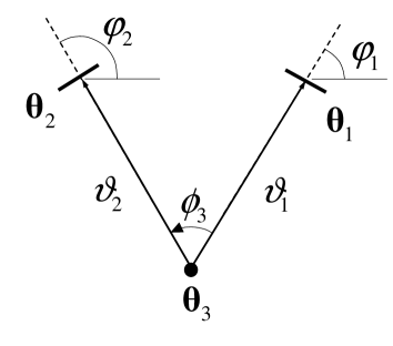
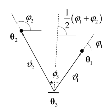
Figure 2: Geometry of the galaxy-shear-shear correlation, $G_{\pm}(\vartheta_{1},\vartheta_{2},\phi_{3})$ (left panel), and the galaxy-galaxy-shear correlation, ${\cal G}(\vartheta_{1},\vartheta_{2},\phi_{3})$ (right panel). The figure is copied from Schneider & Watts (2005).

For our analysis we consider two different classes of correlation functions. Both classes require triplets of galaxies which are located at the positions $\@vec{\theta}_{1}$, $\@vec{\theta}_{2}$ and $\@vec{\theta}_{3}$ on the sky (see Fig. 2). In a cosmological context, random fields – such as the projected number density of galaxies, $N(\@vec{\theta})$, or the shear field, $\gamma(\@vec{\theta})$ – are statistically homogeneous and isotropic. For that reason, all conceivable correlations between the values of those fields depend merely on the separation, $|\@vec{\theta}_{i}-\@vec{\theta}_{j}|$, and never on absolute positions $\@vec{\theta}_{i}$. Therefore, our correlators are solely functions of the dimensions of the triangle formed by the galaxies. We parameterise the dimension of a triangle in terms of the lengths of two triangle edges, $\vartheta_{1}$ and $\vartheta_{2}$, and one angle, $\phi_{3}$, that is subtended by the edges. Note that the sign of $\phi_{3}$, i.e. the handedness of the triangle, is important.

The galaxy-galaxy-shear correlator,

$${\cal G}(\vartheta_{1},\vartheta_{2},\phi_{3})=\left\langle\kappa_{\rm g}(\@vec{\theta}_{1})\kappa_{\rm g}(\@vec{\theta}_{2})\gamma\left(\@vec{\theta}_{3};\frac{\varphi_{1}+\varphi_{2}}{2}\right)\right\rangle\;,$$ (1)

is the expectation value of the shear at $\@vec{\theta}_{3}$ rotated in the direction of the line bisecting the angle $\phi_{3}$ multiplied by the number density contrast of lens (foreground) galaxies at $\@vec{\theta}_{1,2}$:

$$\kappa_{\rm g}(\@vec{\theta})\equiv\frac{N(\@vec{\theta})}{\overline{N}}-1\;.$$ (2)

A rotation of shear is defined as

$$\gamma\left(\@vec{\theta};\varphi\right)\equiv-{\rm e}^{-2{\rm i}\varphi}\gamma_{\rm c}(\@vec{\theta})\;,$$ (3)

where $\gamma_{\rm c}$ is the shear relative to a Cartesian coordinate frame. It should be noted that $\cal G$ and the following correlators are complex numbers.

A second class of correlators are the galaxy-shear-shear correlators,

$$G_{+}(\vartheta_{1},\vartheta_{2},\phi_{3}) = \left\langle\gamma(\@vec{\theta}_{1};\varphi_{1})\gamma^{\ast}(\@vec{\theta}_{2};\varphi_{2})\kappa_{\rm g}(\@vec{\theta}_{3})\right\rangle\;,$$

$$G_{-}(\vartheta_{1},\vartheta_{2},\phi_{3}) = \left\langle\gamma(\@vec{\theta}_{1};\varphi_{1})\gamma(\@vec{\theta}_{2};\varphi_{2})\kappa_{\rm g}(\@vec{\theta}_{3})\right\rangle\;,$$ (4)

which correlate the shear at two points with the lens galaxy number density contrast at another point. Again, the shears are rotated, this time in the direction of the lines connecting the source (background) galaxies, at $\@vec{\theta}_{1,2}$, and the lens galaxy at $\@vec{\theta}_{3}$.

3.2 Practical estimators of correlators

With practical estimators for (1) and (4) in mind, Schneider & Watts (2005) introduced modified correlation functions. They differ from $\cal G$ and $G_{\pm}$ in that they are defined in terms of the number density of the lens galaxies, $N(\@vec{\theta})$, instead of the number density contrast, $\kappa_{\rm g}$:

$$\tilde{\cal G}(\vartheta_{1},\vartheta_{2},\phi_{3})\equiv\frac{\left\langle N(\@vec{\theta}_{1})N(\@vec{\theta}_{2})\gamma\left(\@vec{\theta}_{3};\frac{\varphi_{1}+\varphi_{2}}{2}\right)\right\rangle}{\overline{N}^{2}}$$

$$={\cal G}(\vartheta_{1},\vartheta_{2},\phi_{3})+\left\langle\gamma_{\rm t}\right\rangle(\vartheta_{1}){\rm e}^{-{\rm i}\phi_{3}}+\left\langle\gamma_{\rm t}\right\rangle(\vartheta_{2}){\rm e}^{+{\rm i}\phi_{3}}\;,$$

and

$$\tilde{G}_{+}(\vartheta_{1},\vartheta_{2},\phi_{3})\equiv\frac{1}{\overline{N}}\left\langle\gamma(\@vec{\theta}_{1};\varphi_{1})\gamma^{\ast}(\@vec{\theta}_{2};\varphi_{2})N(\@vec{\theta}_{3})\right\rangle$$ (6)

$$=G_{+}(\vartheta_{1},\vartheta_{2},\phi_{3})+\left\langle\gamma(\@vec{\theta}_{1};\varphi_{1})\gamma^{\ast}(\@vec{\theta}_{2};\varphi_{2})\right\rangle\;,$$

$$\tilde{G}_{-}(\vartheta_{1},\vartheta_{2},\phi_{3})\equiv\frac{1}{\overline{N}}\left\langle\gamma(\@vec{\theta}_{1};\varphi_{1})\gamma(\@vec{\theta}_{2};\varphi_{2})N(\@vec{\theta}_{3})\right\rangle$$ (7)

$$=G_{-}(\vartheta_{1},\vartheta_{2},\phi_{3})+\left\langle\gamma(\@vec{\theta}_{1};\varphi_{1})\gamma(\@vec{\theta}_{2};\varphi_{2})\right\rangle\;.$$

These correlators also contain, apart from the original purely $3^{\rm rd}$-order contributions, contributions from $2^{\rm nd}$-order correlations: $\left\langle\gamma_{\rm t}\right\rangle(\theta)$ is the mean tangential shear about a single lens galaxy at separation $\theta$ (GGL), $\left\langle\gamma(\@vec{\theta}_{1};\varphi_{1})\gamma^{\ast}(\@vec{\theta}_{2};\varphi_{2})\right\rangle$ and $\left\langle\gamma(\@vec{\theta}_{1};\varphi_{1})\gamma(\@vec{\theta}_{2};\varphi_{2})\right\rangle$ are shear-shear correlations which are functions of the cosmic-shear correlators $\xi_{\pm}(\theta)$ (e.g. Bartelmann & Schneider 2001). To recover pure $3^{\rm rd}$-order statistics, the $2^{\rm nd}$-order terms can either be subtracted, or even neglected, if we work in terms of the aperture statistics, as we will see in the next section.

With respect to practical estimators, number densities are more useful quantities because every single galaxy position is an unbiased estimator of $N(\@vec{\theta})/\overline{N}$. For that reason, every triangle of galaxies that can be found in a survey can be made an unbiased estimator of either $\tilde{\cal G}$ (two lenses and one source) or $\tilde{G}_{\pm}$ (two sources and one lens). Since, generally, a weighted average of (unbiased) estimates is still an (unbiased) estimate, we can combine the estimates of all triangles of the same dimension using arbitrary weights, $w_{j/k}$, for the sources. Note that for the following sums only triangles of the same $\vartheta_{1}$, $\vartheta_{2}$ and $\phi_{3}$ have to be taken into account inside the sums. We adopt a binning such that $\vartheta_{1}$, $\vartheta_{2}$ and $\phi_{3}$ need to be within some binning interval to be included inside the sums, i.e. triangles of similar dimensions are used for the averaging:

$$\tilde{G}^{\rm est}_{+} = \frac{\sum\limits_{i,j,k=1}^{N_{\rm l},N_{\rm s}}w_{j}\,w_{k}\,\epsilon_{j}\epsilon_{k}^{\ast}{\rm e}^{-2{\rm i}\varphi_{j}}{\rm e}^{+2{\rm i}\varphi_{k}}}{\sum\limits_{i,j,k=1}^{N_{\rm l},N_{\rm s}}w_{j}\,w_{k}}\;,$$ (8)

$$\tilde{G}^{\rm est}_{-} = \frac{\sum\limits_{i,j,k=1}^{N_{\rm l},N_{\rm s}}w_{j}\,w_{k}\,\epsilon_{j}\epsilon_{k}{\rm e}^{-2{\rm i}\varphi_{j}}{\rm e}^{-2{\rm i}\varphi_{k}}}{\sum\limits_{i,j,k=1}^{N_{\rm l},N_{\rm s}}w_{j}\,w_{k}}\;,$$ (9)

where $j,k\in\{1\ldots N_{\rm s}\}$ are indices for sources and $i\in\{1\ldots N_{\rm l}\}$ is the index of the lenses; $N_{\rm l}$ and $N_{\rm s}$ are the number of lenses and sources, respectively. By $\varphi_{j}$ and $\varphi_{k}$ we denote the phase angles of the two sources relative to the foreground galaxy $i$.

The statistical weights are chosen to down-weight triangles that contain sources whose complex ellipticities, $\epsilon_{i}$ (Bartelmann & Schneider 2001), are only poorly determined. Lenses, however, always have the same weight in our analysis.

Similarly, we can define an estimator for $\tilde{\cal G}$. However, one has to take into account that $\epsilon\,{\rm e}^{-{\rm i}(\varphi_{1}+\varphi_{2})}$ of one single triangle – consisting of two lenses and one source with ellipticity $\epsilon$ – is an estimator of

$$\frac{\left\langle N(\@vec{\theta}_{1})N(\@vec{\theta}_{2})\gamma\left(\@vec{\theta}_{3};\frac{\varphi_{1}+\varphi_{2}}{2}\right)\right\rangle}{\left\langle N(\@vec{\theta}_{1})N(\@vec{\theta}_{2})\right\rangle}=\frac{\tilde{\cal G}(\vartheta_{1},\vartheta_{2},\phi_{3})}{1+\omega(|\@vec{\theta}_{2}-\@vec{\theta}_{1}|)}$$ (10)

and not $\tilde{\cal G}$ alone as has falsely been assumed in Schneider & Watts (2005). The function

$$\omega(|\@vec{\Delta\theta}|)\equiv\left\langle\kappa_{\rm g}(\@vec{\theta})\kappa_{\rm g}(\@vec{\theta}+\@vec{\Delta\theta})\right\rangle$$ (11)

is the angular clustering of the lenses (Peebles 1980). Based on this notion, we can write down an estimator for $\tilde{\cal G}$:

$$\tilde{\cal G}^{\rm est}=\frac{\sum\limits_{i,j,k=1}^{N_{\rm l},N_{\rm s}}w_{k}\,\epsilon_{k}\,{\rm e}^{-{\rm i}(\varphi_{i}+\varphi_{j})}\left[1+\omega(|\@vec{\theta}_{i}-\@vec{\theta}_{j}|)\right]}{(-1)\,\sum\limits_{i,j,k=1}^{N_{\rm l},N_{\rm s}}w_{k}}$$ (12)

that includes explicitly the clustering of lenses. Here, $w_{k}$ ($k\in\{1\ldots N_{\rm s}\}$) are the statistical weights of the sources. By $\varphi_{i}$ and $\varphi_{j}$ ($i,j\in\{1\ldots N_{\rm l}\}$) we denote the phase angles of the two lenses relative to the source $k$. Again, only triangles of the same or similar dimensions (parameters in same bins) are to be included inside the sums.

For obtaining an estimate of $\omega(\theta)$ in practice we employed the estimator of Landy & Szalay (1993), which, compared to other estimators, minimises the variance to nearly Poissonian:

$$\omega\left(\theta\right)=\frac{DD}{RR}-2\frac{DR}{RR}+1\;.$$ (13)

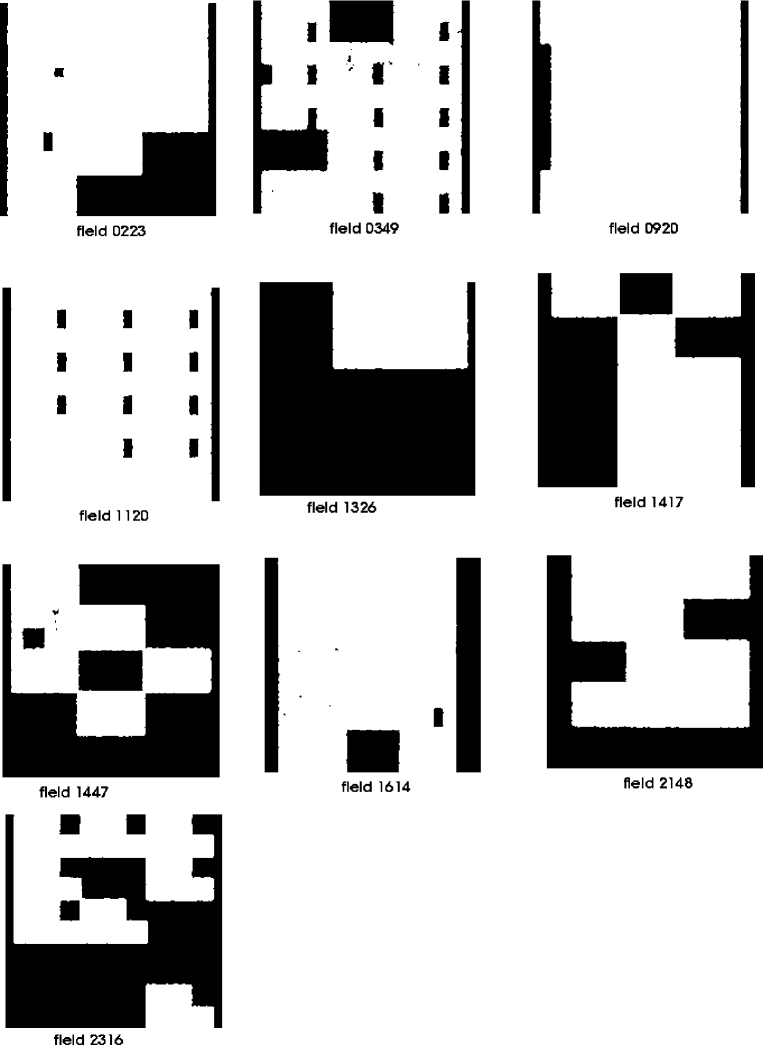
Figure 12: Determined geometry of the individual RCS fields (field masks). Each mask has a size of approximately $139^{\prime}\times 139^{\prime}$ or, equivalently, $20.000\times 20.000\leavevmode\nobreak\ \rm pixel^{2}$. Black colours denote masked-out regions, while white indicates regions where galaxies have been found.

It requires one to count the number of (lens) galaxy pairs with a separation between $\theta$ and $\theta+\delta\theta$, namely the number of pairs in the data, denoted by $DD$, the number of pairs in a random mock catalogue, $RR$, and the number of pairs that can be formed with one data galaxy and one mock data galaxy, $DR$. The random mock catalogue is computed by randomly placing the galaxies, taking into account the geometry of the data field, i.e. by avoiding masked-out regions, see Fig. 12. We generate $25$ random galaxy catalogues and average the pair counts obtained for $DR$ and $RR$.

When computing the $\tilde{\cal G}$ and $\tilde{G}_{\pm}$ estimators, we suggest the use of complex numbers for the angular positions of galaxies: $\@vec{\vartheta}=\vartheta_{1}+{\rm i}\vartheta_{2}$ with $\vartheta_{1,2}$ being the $x$/$y$-coordinates relative to some Cartesian reference frame (flat-sky approximation). The phase factors turning up inside the sums (8), (9) and (12) are then simply (notation of Fig. 2):

$${\rm e}^{-2{\rm i}\varphi_{1}}=\frac{\@vec{\vartheta}^{\ast}_{13}}{\@vec{\vartheta}_{13}}\,;\,{\rm e}^{-2{\rm i}\varphi_{2}}=\frac{\@vec{\vartheta}^{\ast}_{23}}{\@vec{\vartheta}_{23}}\,;\,{\rm e}^{-{\rm i}(\varphi_{1}+\varphi_{2})}=\frac{\@vec{\vartheta}_{13}\@vec{\vartheta}_{23}}{|\@vec{\vartheta}_{13}||\@vec{\vartheta}_{23}|}\;,$$ (14)

where $\@vec{\vartheta}_{ij}\equiv\@vec{\vartheta_{i}}-\@vec{\vartheta}_{j}$.

3.3 Conversion to aperture statistics

In weak lensing, cosmological large-scale structure is often studied in terms of the aperture statistics (Simon et al. 2007; Kilbinger & Schneider 2005; Jarvis et al. 2004; Hoekstra et al. 2002a; Schneider 1998; Van Waerbeke 1998) that measure the convergence (projected matter distribution), $\kappa$, and projected number density fields of galaxies, $\kappa_{\rm g}$, smoothed with a compensated filter $u(x)$, i.e. $\int_{0}^{\infty}{\rm d}x\,xu(x)=0$:

$$M_{\rm ap}(\theta) = \frac{1}{\theta^{2}}\int_{0}^{\infty}\,{\rm d}^{2}\vartheta\,u\!\left(\frac{|\@vec{\vartheta}|}{\theta}\right)\,\kappa(|\@vec{\vartheta}|)\;,$$ (15)

$${\cal N}(\theta) = \frac{1}{\theta^{2}}\int_{0}^{\infty}\,{\rm d}^{2}\vartheta\,u\!\left(\frac{|\@vec{\vartheta}|}{\theta}\right)\,\kappa_{\rm g}(|\@vec{\vartheta}|)\;,$$ (16)

where $\theta$ is the smoothing radius. $M_{\rm ap}$ is called the aperture mass, while ${\cal N}$ is the aperture number count of galaxies. With an appropriate filter these aperture measures are only sensitive to a very narrow range of spatial Fourier modes so that they are extremely suitable for studying the scale-dependence of structure, or even the scale-dependence of remaining systematics in the data (Hetterscheidt et al. 2007). Moreover, they provide a very localised measurement of power spectra (band power), in the case of $\left\langle{\cal N}^{n}M_{\rm ap}^{m}\right\rangle$ for $n+m=2$, and bispectra, in the case of $n+m=3$, without relying on complicated transformations between correlation functions and power spectra. The aperture filter we employ for this paper is:

$$u(x)=\frac{1}{2\pi}\left(1-\frac{x^{2}}{2}\right){\rm e}^{-x^{2}/2}$$ (17)

as introduced by Crittenden et al. (2002). For an aperture radius of $\theta$ the filter peaks at a spatial wavelength of $\ell=\frac{\sqrt{2}}{\theta}$ which corresponds to a typical angular scale of $\frac{2\pi}{\ell}=\frac{\pi}{\sqrt{2}}\theta$.

As shear and convergence are both linear combinations of second derivatives of the deflection potential, the aperture mass can be computed from the shear in the following manner (Schneider et al. 1998):

$$M_{\rm ap}(\theta)+{\rm i}M_{\perp}(\theta) = \frac{1}{\theta^{2}}\int_{0}^{\infty}\!\!\!\!{\rm d}^{2}\@vec{\theta}^{\prime}\,q\left(\frac{|\@vec{\theta}^{\prime}|}{\theta}\right)\gamma\left(\@vec{\theta}^{\prime};\angle\@vec{\theta}^{\prime}\right)\!\!\;,$$ (18)

$$q(x) \equiv \frac{2}{x^{2}}\int_{0}^{x}{\rm d}s\,s\,u(s)-u(x)\;,$$ (19)

where we denote by $\angle\@vec{\theta}^{\prime}$ the polar angle of the vector $\@vec{\theta}^{\prime}$. Note that in Eq. (18) we place, for convenience, the origin of the coordinate system at the centre of the aperture.

In expression (18), $M_{\rm ap}$ is the E-mode, whereas $M_{\perp}$ is the B-mode of the aperture mass. Of central importance for our work is that we can extract E- and B-modes of the aperture statistics from the correlation functions. Since B-modes cannot be generated by weak gravitational lensing, a zero or small B-mode is an important check for a successful PSF-correction of real data (e.g. Hetterscheidt et al. 2007), or the violation of parity-invariance in the data (Schneider 2003), which is also a signature of systematics.

Another argument in favour of using aperture statistics at this stage of our analysis is that $2^{\rm nd}$-order terms in $\tilde{\cal G}$ and $\tilde{G}_{\pm}$ do not contribute to the $3^{\rm rd}$-order aperture statistics (Schneider & Watts 2005). Therefore, a significant signal in the aperture statistics means a true detection of $3^{\rm rd}$-order correlations.

The $3^{\rm rd}$-order aperture statistics can be computed from $\tilde{\cal G}$ via:

$$\left\langle{\cal N}^{2}M_{\rm ap}\right\rangle(\theta_{1},\theta_{2},\theta_{3})=$$ (20)

$$\Re{\left({\cal I}\left[\tilde{\cal G}(\vartheta_{1},\vartheta_{2},\phi_{3})A_{{\cal N}{\cal N}M}(\vartheta_{1},\vartheta_{2},\phi_{3}|\theta_{1},\theta_{2},\theta_{3})\right]\right)}\;,$$

$$\left\langle{\cal N}^{2}M_{\perp}\right\rangle(\theta_{1},\theta_{2},\theta_{3})=$$ (21)

$$\Im{\left({\cal I}\left[\tilde{\cal G}(\vartheta_{1},\vartheta_{2},\phi_{3})A_{{\cal N}{\cal N}M}(\vartheta_{1},\vartheta_{2},\phi_{3}|\theta_{1},\theta_{2},\theta_{3})\right]\right)}\;,$$

where we have introduced for the sake of brevity an abbreviation for the following integral:

$${\cal I}\left[f\right]\equiv\int\limits_{0}^{\infty}{\rm d}\vartheta_{1}\vartheta_{1}\int\limits_{0}^{\infty}{\rm d}\vartheta_{2}\vartheta_{2}\int\limits_{0}^{2\pi}{\rm d}\phi_{3}\,\,f\;.$$ (22)

By $\Re{(x)}$ and $\Im{(x)}$ we denote the real and imaginary part, respectively, of a complex number $x$. Eq. (20) is the E-mode of the aperture moment $\left\langle{\cal N}(\theta_{1}){\cal N}(\theta_{2})M_{\rm ap}(\theta_{3})\right\rangle$, whereas Eq. (21) is the corresponding parity mode that is non-zero in the case of violation of parity-invariance; the latter has to be zero even if B-modes are present in the shear pattern that may be produced to some degree by intrinsic source alignment (e.g. Heymans et al. 2004) or intrinsic ellipticity/shear correlations (Hirata & Seljak 2004) – that is, if we assume that the macroscopic world is parity-invariant. The integral kernel $A_{{\cal N}{\cal N}M}$ for our aperture filter can be found in the Appendix of Schneider & Watts (2005).

The aperture statistics associated with the GGGL-correlator $\tilde{G}_{\pm}$ are the following:

$$\left\langle M_{\rm ap}^{2}{\cal N}\right\rangle(\theta_{1},\theta_{2},\theta_{3})=$$ (23)

$$\Re{\left[\left\langle MM{\cal N}\right\rangle(\theta_{1},\theta_{2},\theta_{3})+\left\langle MM^{\ast}{\cal N}\right\rangle(\theta_{1},\theta_{2},\theta_{3})\right]}/2\;,$$

$$\left\langle M_{\perp}^{2}{\cal N}\right\rangle(\theta_{1},\theta_{2},\theta_{3})=$$ (24)

$$\Re{\left[\left\langle MM^{\ast}{\cal N}\right\rangle(\theta_{1},\theta_{2},\theta_{3})-\left\langle MM{\cal N}\right\rangle(\theta_{1},\theta_{2},\theta_{3})\right]}/2\;,$$

$$\left\langle M_{\perp}M_{\rm ap}{\cal N}\right\rangle(\theta_{1},\theta_{2},\theta_{3})=$$ (25)

$$\Im{\left[\left\langle MM{\cal N}\right\rangle(\theta_{1},\theta_{2},\theta_{3})+\left\langle MM^{\ast}{\cal N}\right\rangle(\theta_{1},\theta_{2},\theta_{3})\right]}/2\;,$$

where we used the following definitions

$$\left\langle MM{\cal N}\right\rangle(\theta_{1},\theta_{2},\theta_{3})\equiv$$ (26)

$${\cal I}\left[\tilde{G}_{-}(\vartheta_{1},\vartheta_{2},\phi_{3})A_{MM{\cal N}}(\vartheta_{1},\vartheta_{2},\phi_{3}|\theta_{1},\theta_{2},\theta_{3})\right]\;,$$

$$\left\langle MM^{\ast}{\cal N}\right\rangle(\theta_{1},\theta_{2},\theta_{3})\equiv$$ (27)

$${\cal I}\left[\tilde{G}_{+}(\vartheta_{1},\vartheta_{2},\phi_{3})A_{MM^{\ast}{\cal N}}(\vartheta_{1},\vartheta_{2},\phi_{3}|\theta_{1},\theta_{2},\theta_{3})\right]\;.$$

Eq. (23) is the E-mode of $\left\langle M_{\rm ap}(\theta_{1})M_{\rm ap}(\theta_{2}){\cal N}(\theta_{3})\right\rangle$, Eq. (24) is the B-mode which should vanish if the shear pattern is purely gravitational, and Eq. (25) is again a parity-mode which is a unique indicator for systematics. As before, the integral kernels $A_{MM{\cal N}}$ and $A_{MM^{\ast}{\cal N}}$ for our aperture filter may be found in the Appendix of Schneider & Watts (2005).

3.4 Validating the code

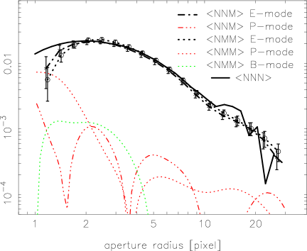
Figure 3: Test run of our computer code with mock data based on some arbitrary convergence field. The mock data has been prepared such that $\left\langle{\cal N}^{2}(\theta)M_{\rm ap}(\theta)\right\rangle=\left\langle{\cal N}(\theta)M^{2}_{\rm ap}(\theta)\right\rangle=\left\langle{\cal N}^{3}(\theta)\right\rangle$; $\left\langle NNN\right\rangle\equiv\left\langle{\cal N}^{3}(\theta)\right\rangle$ is the value that has to be found by the code (only equally sized apertures are correlated for test: $\theta_{1}=\theta_{2}=\theta_{3}=\theta$). The binning range is between $\vartheta\in[0.05,200]\leavevmode\nobreak\ \rm pixel$ with $100$ bins; we use $10^{4}$ lenses and the same number of sources. For radii greater than $\sim\!2$ pixel we get good agreement. The expected signal (solid line; computed from placing apertures) becomes inaccurate beyond $\theta\gtrsim 10$ pixel because the aperture size becomes comparable to the field size. The error bars denote the $1\sigma$ sampling uncertainty due to finite galaxy numbers. The B- and parity modes (P) of the statistics are two orders of magnitude smaller than the E-modes and are oscillating about zero (plotted is modulus).

In the last section, we outlined the steps which have to be undertaken in order to estimate the $3^{\rm rd}$-order aperture moments from a given catalogue of lenses and sources. The three steps are: 1) estimating the angular clustering of lenses yielding $\omega(\theta)$, 2) estimating $\tilde{\cal G}$ and $\tilde{G}_{\pm}$ for some range of $\vartheta_{1,2}$ and for $\phi_{3}\in[0,2\pi[$, and finally 3) transforming the correlation function to $\left\langle{\cal N}^{2}M_{\rm ap}\right\rangle$ and $\left\langle{\cal N}M^{2}_{\rm ap}\right\rangle$ including all E-, B- and parity-modes.

There are several practical issues involved here. One issue is that, in theory, for the transformation we require $\tilde{\cal G}$, $\tilde{G}_{\pm}$ for all $\vartheta\in[0,\infty]$, see Eq. (22). In reality, we will have both a lower limit (seeing, galaxy-galaxy overlapping), $\vartheta_{\rm low}$, and an upper limit (finite fields), $\vartheta_{\rm upper}$. On the other hand, the GGGL-correlators drop off quickly for large $\vartheta$ and the integral kernels $A_{{\cal N}{\cal N}M}$, $A_{MM{\cal N}}$, $A_{MM^{\ast}{\cal N}}$ have exponential cut-offs for $\vartheta_{1},\vartheta_{2}\gg\theta_{1,2,3}$. Therefore, we can assume that there will be some range where we can compute the aperture statistics with satisfactory accuracy. We perform the following test to verify that this is true: by using theoretical 3D-bispectra of the galaxy-dark matter cross-correlations (Watts & Schneider 2005) we compute both the GGGL-correlation functions and the corresponding aperture statistics (Eqs. 37, 38, 40, 51, 52 of Schneider & Watts 2005). By binning the GGGL-correlators we perform the transformation including binning and cut-offs in $\vartheta$. We find that one can obtain an accurate estimate of the aperture statistics within a few percent between roughly $\theta\gtrsim 40\,\vartheta_{\rm low}$ and $\theta\lesssim\vartheta_{\rm upper}/10$ (using $100$ log-bins for $\vartheta_{1,2}$ and $100$ linear bins for $\phi_{3}$). Therefore, with RCS-fields of typical size $139^{\prime}$ we can expect to get an accurate result between about $0^{\prime}\!.5\lesssim\theta\lesssim 14^{\prime}$.

Another issue is with step two above, in which the GGGL-correlators themselves need to be estimated. The estimators – Eqs. (8), (9) and (12) – in terms of galaxy positions and source ellipticities are simple but the enormous number of triangles that need to be considered is computationally challenging (roughly $10^{13}$ per field for RCS). To optimise this process we employ a data structure based on a binary tree, a so-called tree code (e.g. Jarvis et al. 2004; Zhang & Pen 2005). The tree-code represents groups of galaxies within some distance to a particular triangle vertex as “single galaxies” with appropriate weight (and average ellipticity). This strategy effectively reduces the number of triangles. Moreover, we optimise the code such that only distinct triangles are found. Then, the other triangle obtained be exchanging the indices of either the two lenses ($\tilde{\cal G}$) or the two sources ($\tilde{G}_{\pm}$) is automatically accounted for; this reduces the computation time by a factor of two.

In order to test the performance and reliability of the code, we create a catalogue of mock data. In order to do this we use a simulated convergence field ($\kappa$-field) on a grid, $512\times 512\leavevmode\nobreak\ \rm pixel^{2}$, which has been obtained by ray-tracing through an N-body simulated universe. Actually, the only requirement that has to be met by the test field is that it behaves like a density contrast $\delta$, i.e. $\left\langle\delta\right\rangle=0$ and $\delta\geq-1$, and that it has non-vanishing $3^{\rm rd}$-order moments, $\left\langle\delta^{3}\right\rangle\neq 0$. Based on this field we simulate a shear and lens catalogue. The shear catalogue is generated by converting the $\kappa$-field to a shear field and by randomly selecting positions within the field to be used as source positions. The positions and associated shear provide the mock shear catalogue; for details see Simon et al. (2004). In a second step, we use the $\kappa$-field as density contrast, $\kappa_{\rm g}$, of the number density of lenses to make realisations of lens catalogues. This means one randomly draws positions, $\@vec{\theta}$, within the grid area and one accepts that position if $x\leq\frac{1+\kappa(\@vec{\theta})}{1+\kappa_{\rm max}}$, where $x$ is a random number between $x\in[0,1]$ and $\kappa_{\rm max}$ the maximum value within the $\kappa$ field. Following this procedure one gets mock data for which $\kappa=\kappa_{\rm g}$ and therefore $\left\langle{\cal N}^{n}M_{\rm ap}^{m}\right\rangle=\left\langle{\cal N}^{n+m}\right\rangle$. In particular we must get, apart from the statistical noise due to finite galaxy numbers, $\left\langle{\cal N}^{2}(\theta_{1})M_{\rm ap}(\theta_{2})\right\rangle=\left\langle{\cal N}(\theta_{1})M^{2}_{\rm ap}(\theta_{2})\right\rangle$ when running our codes with the mock data.

Parallelly, we smooth the test shear field within apertures according to the definitions (18) with our aperture filter and estimate the test data aperture statistics directly by cross-correlating the smoothed fields. This also has to be comparable (apart from shot noise) to our code output. The result of this test can be found in Fig. 3.

As a further test we take the same mock data but rotate the ellipticities of the sources by $45$ degrees, i.e. we multiply the complex ellipticities by the phase factor $-{\rm e}^{-2{\rm i}\phi}$ with $\phi=45^{\circ}$. This generates a purely B-mode signal that should only be picked up by the B-mode channels of the aperture statistics, yielding a plot similar to Fig. 3. The parity mode in $\left\langle{\cal N}M^{2}_{\rm ap}\right\rangle$ has to be unaffected. This is indeed the case (figure not shown).

The test results make us confident that the computer code is working and that we achieve a good accuracy even though we are forced to bin the correlation functions and to use a tree-code that necessarily makes some additional approximations.

4 Results and discussion

We applied the previously outlined method to the RCS shear and lens catalogues.

Lenses were selected between photometric redshifts $0<z<0.4$, whereas sources were from the range $0.5<z<1.4$. Compared to Hoekstra et al. (2005), in which photometric redshifts smaller than $0.2$ were excluded, we were less strict about the lowest redshift of the lenses. This is likely to have introduced some misidentified lenses into our sample (less than $10\%$, see Fig. 1) as RCS is lacking a U-band filter. Moreover, including sources with photometric redshifts larger than $z\sim 1.0$ is also rather optimistic because photometric redshifts within that range can become quite unreliable as well. Therefore the tail of the redshift distribution in Fig. 1 may be slightly inaccurate. Still, sources with photo-z’s greater than one are likely to be high-redshift galaxies.

However, for our purpose, namely demonstrating a robust detection of GGGL, the biases in the redshift distribution of lenses and sources are acceptable. These biases in the estimated redshift distribution only become an issue if one wants to thoroughly model the GGGL-signal.

Figure 4: Left: Aperture statistics $\left\langle{\cal N}^{2}M_{\rm ap}\right\rangle(\theta,\theta,\theta)$ for different aperture radii $\theta$ as measured in RCS. The upper panel is the E-mode, the lower panel is the parity mode which is consistent with zero. Error bars denote the field-to-field variance between the ten RCS fields. Statistical errors are strongly correlated. The lines are tentative halo model-based predictions with arbitrary HODs for a $\Lambda\rm CDM$ cosmological model (see text). Right: Aperture statistics $\left\langle{\cal N}M_{\rm ap}^{2}\right\rangle(\theta,\theta,\theta)$ for different aperture radii $\theta$ as measured in RCS. The upper panel contains the E-mode measurement, while B-mode (stars) and parity mode (squares) are plotted inside the lower panel. Error bars that extend to the bottom of the upper panel denote data points that are consistent with zero.

4.1 Aperture statistics

Figure 5: Combined measurement of angular clustering of our sample of lenses (no correction for the integral constraint). Error bars were obtained by looking at the field-to-field variance. The solid line is a power-law fit, $\omega(\theta)=A_{\omega}\theta^{-\beta}$, to the regime $\theta\in[0^{\prime}\!.1,3^{\prime}]$.

As a first result we would like to draw the reader’s attention to the angular clustering of lenses which is plotted in Fig. 5. This measurement was required for the estimator $\tilde{\cal G}$ in Eq. (12). As widely accepted, the angular correlation function $\omega(\theta)$ is, for the separations we are considering here, well approximated by a simple power-law, depending on galaxy type, colour and luminosity (e.g. Madgwick et al. 2003). As can be seen in Fig. 5, the power-law behaviour is also found for our lens galaxy sample. The angular clustering plotted is still affected by the so-called integral constraint (Groth & Peebles 1977), which shifts the estimate of $\omega$ downwards by a constant value depending on the geometry and size of the fields. For small $\theta\lesssim 3^{\prime}$ this bias is negligible so that we used only the regime $\theta\in[0^{\prime}\!\!.1,3^{\prime}]$ to find the maximum likelihood parameters of the power-law.

For $\tilde{\cal G}$ this power-law fit was used. Possible deviations of the true clustering from a power-law for $\theta\geq 2^{\prime}$ were negligible because for the estimator one actually needs $1+\omega$ instead of $\omega$. Since $\omega$ is roughly smaller than $\sim 0.05$ and decreasing for $\theta\geq 2^{\prime}$, we gather that a certain remaining inaccuracy in $\omega$ has no big impact on $1+\omega$. The power-law index is, with $\beta=0.58$, fairly shallow, which is typical for a relatively blue sample of galaxies (e.g. Madgwick et al. 2003).

In a second step, the correlation functions $\tilde{\cal G}$ and $\tilde{G}_{\pm}$ were computed separately for each of the ten RCS fields. The total combined signal was computed by taking the average of all fields, each bin weighted by the number of triangles it contained. For the binning we used a range of $0^{\prime\prime}\!.8\leq\vartheta\leq 54^{\prime}$ with $100$ bins, thus overall $10^{6}$ triangle configurations. By repeatedly drawing ten fields at random from the ten available, i.e. with replacement, and combining their signal we obtained a bootstrap sample of measurements. The variance among the bootstrapped signals was used to estimate the sum of cosmic variance and shot noise, thus the remaining statistical uncertainty of the correlation functions.

Figure 6: Residual signal (squares) of GGGL in RCS when the ellipticities of the sources are randomised (left: $\left\langle{\cal N}^{2}M_{\rm ap}\right\rangle$, right: $\left\langle{\cal N}M^{2}_{\rm ap}\right\rangle$). For comparison, the original signal before randomisation is also plotted (crosses). The line is a crude halo-model prediction of a blue galaxy population as in Fig. 4. The error bars of the randomised signal quantify the background noise of a null-signal. This indicates that we have a significant detection of $\left\langle{\cal N}^{2}M_{\rm ap}\right\rangle$ in the left panel but only a weak detection of $\left\langle{\cal N}M_{\rm ap}^{2}\right\rangle$, most significant at about $2^{\prime}$, in the right panel.

Finally, the correlation functions were transformed to the aperture statistics considering only equally sized apertures, i.e. $\theta_{1}=\theta_{2}=\theta_{3}$, see Fig. 4. For the scope of this work, equally sized apertures are absolutely sufficient. In future work, however, one would like to harvest the full information that is contained in these statistics by exploring different $\theta_{i}$ which then would cover the full (projected) bispectrum.

For a start, we would like to focus on $\tilde{\cal G}$. The left panel in Fig. 4 reveals a clean detection of $\left\langle{\cal N}^{2}M_{\rm ap}\right\rangle$ for aperture radii between $0^{\prime}\!\!.5\lesssim\theta\lesssim 5^{\prime}$ (with the adopted filter this corresponds to typical angular scales between $1^{\prime}$ and $11^{\prime}$) demonstrating the presence of pure $3^{\rm rd}$-order correlations between shear and lens distribution in RCS. The parity mode of this statistic is consistent with the zero as expected. Fig. 4 is one of the central results of this paper.

We would like to further support that this is a real, i.e. cosmological, signal by comparing the measurement to crude halo model-based predictions (see Cooray & Sheth 2002, for a review). The halo model was used to predict a spatial cross-correlation bispectrum, $B_{{\rm gg}\delta}$ (Eq. 12 in Schneider & Watts 2005), for a particular fiducial cosmological model and halo occupation distribution (HOD) of galaxies (see Berlind & Weinberg 2002). By applying Eqs. (21), (52) in Schneider & Watts (2005), $B_{{\rm gg}\delta}$ was transformed, taking into account the correct redshift distribution of lenses and sources (Fig. 1), to yield the aperture statistics. A standard concordance $\Lambda\rm CDM$ model was employed (Bardeen et al. 1986) with parameters $\Omega_{\Lambda}=0.7$, for the dark energy density, $\Omega_{\rm m}=0.30$, for the (cold) dark matter density, $\sigma_{8}=0.9$ for the power spectrum normalisation, and $\Gamma=0.21$ for the shape parameter. This is in agreement with constraints based on the first WMAP release (Spergel et al. 2003).

The latest constraints favour a somewhat smaller value for $\sigma_{8}$ (Benjamin et al. 2007; Hetterscheidt et al. 2007) which would shift the expected amplitude of GGGL towards smaller values. If we apply the scaling relation of Jain & Seljak (1997), given for the convergence bispectrum, as a rough estimate of this shift, $B_{\kappa}\propto\sigma_{8}^{5.9}$, we obtain a correction factor of about two for $\sigma_{8}=0.8$ ($\cal N$ and $M_{\rm ap}$ should have the same $\sigma_{8}$-dependence for unbiased galaxies).

The halo-model predictions depend strongly on the adopted HOD. The basic set up for this model was that outlined in Takada & Jain (2003), which splits the occupation function, $N(M)$, into contributions from “red”, $N_{R}$, and “blue”,$N_{B}$, galaxies:

$$\left\langle N_{B}\right\rangle(M) = \left(\frac{m}{m_{B}}\right)^{\gamma_{B}}+{\rm A}\exp{\left(-{\rm A}_{0}(\log_{10}(m)-m_{B_{s}})^{2}\right)}$$

$$\left\langle N_{R}\right\rangle(M) = \left(\frac{m}{m_{R}}\right)^{\gamma_{R}}\exp{\left(-\left[\frac{m_{R_{0}}}{m}\right]^{1,2}\right)}\;.$$ (28)

As parameters we used $m_{B}=2.34\times 10^{13}\,{\rm M}_{\odot}$, ${\rm A}=0.65$, ${\rm A}_{0}=6.6$, $m_{B_{s}}=11.73$, $m_{R}=1.8\times 10^{13}\,{\rm M}_{\odot}$ and $m_{R_{0}}=4.9\times 10^{12}\,{\rm M}_{\odot}$. Blue galaxies have a peak halo occupancy of around $10^{12}\,{\rm M}_{\odot}$ and a shallow power law ($\gamma_{B}=0.93$) at high halo masses. In this simple prescription, red galaxies are relatively more numerous in higher mass halos ($\gamma_{R}=1.1$) and are excluded from low mass halos by an exponential cutoff around $5\times 10^{12}\,{\rm M}_{\odot}$. Factorial moments of the occupation distribution - the cross bisprectra $B_{gg\delta}$ and $B_{\delta\delta g}$ require the mean and variance - were as prescribed in the model of Scoccimarro et al. (2001). In this way, the moments are Poissonian for higher mass halos, becoming sub-Poissonian for masses below $10^{13}\,{\rm M}_{\odot}$, i.e. $\left\langle N^{2}\right\rangle(M)=\alpha^{2}[\left\langle N\right\rangle(M)]^{2}$, where $\alpha=0.5\log_{10}{(m/10^{11}\,{\rm M}_{\odot})}$.

We stress at this point that we made no attempt to “fit” parameters to the data, we merely intended to bracket a range of possible results. To choose a range of plausible scenarios, we constructed the theoretical aperture statistics for “red” galaxies, “blue” galaxies and for “all” galaxies (in which the occupation functions for red and blue galaxies are added together directly). We also showed predictions for the unbiased case, in which the occupation function $N(M)\propto M$ with Poisson moments for $\left\langle N^{2}(M)\right\rangle$. Galaxies were assumed to follow the CDM halo density profile (NFW) with no assumption of a central galaxy. Other parameters that define the halo model set up (e.g. concentration of the NFW profile) were as used in Takada & Jain (2003).

Our measurement of $\left\langle{\cal N}^{2}M_{\rm ap}\right\rangle$ lies somewhat above the lower bound of the expected physical range of values, giving support as to the cosmological origin of the signal. Moreover, taken at face value, our result appears to fit the picture that the lens population consists of rather blue galaxies as has been concluded from the shallow slope of the angular correlation function $\omega$.

We randomised the ellipticities of the sources and repeated the analysis. Since the coherent pattern, and its correlation to the lens distribution, is responsible for the signal, destroying the coherence by randomising the ellipticity phase should diminish the signal. That this is the case can be seen in Fig. 6 (left panel).

Analogous to $\left\langle{\cal N}^{2}M_{\rm ap}\right\rangle$ we computed and predicted $\left\langle{\cal N}M_{\rm ap}^{2}\right\rangle$, the result for which is shown in Fig. 4 (right panel). Here a signal significantly different from zero was only found for aperture radii $1^{\prime}\leq\theta\leq 3^{\prime}$ and at about $\theta\sim 0^{\prime}\!\!.5$. Below $\theta\sim 1^{\prime}\!\!.5$ the parity mode is not fully consistent with zero. Hence, we may have a non-negligible contamination by systematics in the PSF correction and/or intrinsic alignments of the sources that may hamper a clean detection. For radii where we find a non-zero signal, the signal is on average smaller than the lowest theoretical value from our crude models. However, as discussed above, a lower $\sigma_{8}$ easily brings the model down towards smaller values. The signal disappeared if the ellipticities of the sources were randomised (Fig. 6, right panel). Therefore, we found a tentative detection of $\left\langle{\cal N}M_{\rm ap}^{2}\right\rangle$ in our data.

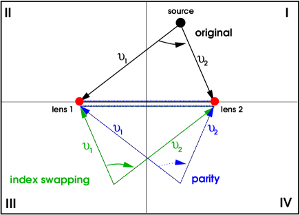
Figure 7: Sketch illustrating how $\tilde{\cal G}$ or $\cal G$ are plotted. See text for details.

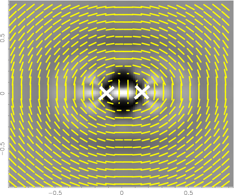
Figure 8: Signal in $\tilde{\cal G}$ originating from pure $2^{\rm nd}$-order statistics (GGL) that was subtracted from $\tilde{\cal G}$ to obtain Fig. 9 (left). The gray-scale intensity is the modulus of $\tilde{\cal G}$, the sticks indicate the average shear at the source position in the lens-lens-source triangle configuration. The units of the axis are in $h^{-1}\rm Mpc$ which corresponds to the mean physical scale at the lens distance of about $z=0.30$. The two lenses are located at the positions of the crosses, left and right from the centre.

4.2 Mapping the excess matter distribution about two lenses

The aperture statistics clearly have advantages: the B- and parity-modes allow a check for remaining systematics in the data, and $2^{\rm nd}$-order statistics do not make any contributions so that we can be sure to pick up a signal solely from connected $3^{\rm rd}$-order terms. This is what we did in the forgoing subsection. The result suggests that we have a significant detection of $\cal G$.

The disadvantage of using aperture statistics is, however, that they are hard to visualise in terms of a typical (projected) matter distribution (lensing convergence) about two lenses, say. Therefore, we introduce here an alternative way of depicting $\cal G$ which is similar to the work that has been proposed by Johnston (2006).

A similar way of visualising $G_{\pm}$ probably could be thought up as well. However, since we found only a weak detection of GGGL with two sources and one lens we postpone this task to a future paper and focus here on $\cal G$ alone.

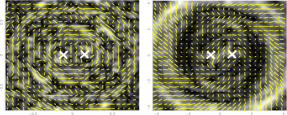
Figure 9: Plots of $\cal G$ after subtraction of the $2^{\rm nd}$-order signal from $\tilde{\cal G}$. The units used are $h^{-1}\rm Mpc$, which corresponds to the mean comoving physical distance at the lenses’ distance of, on average, $z=0.30$. Left: Lenses were selected to have a mutual angular separation between $40^{\prime\prime}$ and $80^{\prime\prime}$ corresponding a projected physical scale of about $250\,h^{-1}\rm kpc$. Right: Lenses were chosen to have a separation between $4^{\prime}$ and $8^{\prime}$, or equivalently a projected comoving separation between $1-2\,h^{-1}\rm Mpc$.

The following summarises what essentially is done if we estimate $\tilde{\cal G}$ from the data for fixed lens-lens separations. We pick out only lens-lens-source triangles from our data set in which the lenses have a fixed separation or a separation from a small range. Each triangle is placed inside the plot such that the line connecting the lenses is parallel to the $x$-axis and that the centre of this line coincides with the centre of the plot, as seen for the triangles in Fig. 7. The ellipticities of the sources of all triangles are then multiplied by $1+\omega(|\theta_{2}-\theta_{1}|)$ (rescaled according to Eq. 10) and (weighted) averaged at the source positions. For this paper, we used $128\times 128$ grid cells for binning the ellipticities. Following this procedure we effectively stacked all shear patterns about a lens-lens configuration – rotated appropriately – to obtain an average shear field about two lenses. This is, in essence, the meaning of $\tilde{\cal{G}}$. The full $\tilde{\cal G}$ is a bundle of such plots with continuously changing lens-lens separations.

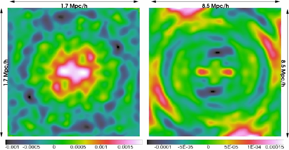
Figure 10: Convergence fields obtained by transforming the shear fields in Fig. 9. They are related to the (average) excess in matter density around two galaxies of fixed angular separation after subtraction of the matter density profile that is observed about individual galaxies. Left: Residual convergence for two lenses with projected comoving distance of roughly $250\,h^{-1}\rm kpc$. The box-size is $1.7\,h^{-1}{\rm Mpc}\times 1.7\,h^{-1}{\rm Mpc}$. Right: Residual convergence at about $1.5\,h^{-1}\rm Mpc$ projected lens-lens distance. The box-size is $8.5\,h^{-1}{\rm Mpc}\times 8.5\,h^{-1}{\rm Mpc}$. Note that the convergence in this figure is lower by roughly an order of magnitude compared to the left figure.

Note that the ellipticity at the source position, stored in $\cal G$, is rotated by $\phi_{3}/2$ (Fig. 2, right panel). For the following plots, on the other hand, we used the shear in Cartesian coordinates relative to axis defined by the lens positions, as in Johnston (2006). Therefore, when generating the plot we were rotating our measurements for $\tilde{\cal G}$ appropriately.

The resulting plot has symmetries. Firstly, we do not distinguish between ”lens 1” and “lens 2”. Both lenses are drawn from the same galaxy sample. This means for every triangle, we will find the same triangle but with the positions of “lens 1” and “lens 2” exchanged. Therefore, the two lenses and the source of the triangle named “original” in Fig. 7 will make the same contribution but complex conjugated at the source position of the triangle named “index swapping”. Thus, quadrants I and III will be identical apart from a complex conjugate and mirroring the positions about the $x$- and $y$-axis. The same holds for quadrants II and IV. This would no longer be true, of course, if we chose the two lenses from different catalogues in order to, for instance, study the matter distribution around a blue and a red galaxy.

A second symmetry can be observed if the Universe (or the PSF-corrected shear catalogue) is parity invariant. Mirroring the triangle “original” with respect to the line connecting the two lenses ($x$-axis) results in another triangle coined “parity”. For parity invariance being true the ellipticity at the source position of “parity” is on average identical to the ellipticity at the source position of triangle “original”. In this case, quadrant IV is statistically consistent with quadrant I and quadrant II with quadrant III (after mirroring about the $x$-axis). Taking parity symmetry for granted could be used to increase the signal-to-noise in the plots by taking the mean of quadrants IV and I (or II and III).

Since the way of binning in the plot is completely different from the way used to get the aperture statistics out of RCS, we made two reruns of the estimation of $\tilde{\cal G}$ with our data. For the first run we only considered lens-lens separations between $40^{\prime\prime}$ and $80^{\prime\prime}$, the second run selected triangles in which the lenses had a separation between $4^{\prime}$ and $8^{\prime}$. For a mean lens redshift of $z\sim 0.3$ this corresponds to a projected physical comoving separation of roughly $250\,h^{-1}\rm kpc$ and $1.5\,h^{-1}\rm Mpc$, respectively. As usual, the results from the ten individual fields were averaged by weighting with the number of triangles inside each bin and the statistical weights of the sources.

Since we effectively stacked the shear fields about all pairs of lenses, aligned along the lens-lens axis, we obtained the average shear about two lenses. The shear pattern still contained a contribution stemming from GGL alone. This contribution could, however, easily be subtracted according to Eq. (3.2) after estimating the mean tangential shear, $\left\langle\gamma_{\rm t}\right\rangle(\vartheta)$, about single lens galaxies (see e.g. Simon et al. 2007). A typical shear pattern due to $2^{\rm nd}$-order GGL can be seen in Fig. 8. This is the shear pattern that is to be expected if the average shear about two lenses is just the sum of two mean shear patterns about individual lenses. They contain all contributions that are statistically independent of the presence of the other lens. Therefore, contributions (contaminations) to the shear from lens pairs that are just accidentally close to each other by projection effects, but actually too separated in space to be physically connected, are removed.

Now, Fig. 9 shows the shear patterns after removing this signal. Clearly, there is a residual coherent pattern which is most pronounced for the smaller lens-lens separations. This proves that one finds an additional shear signal around two galaxies if they get close to each other. Hence, the average gravitational potential about two close lenses is not just the sum of two average potentials about individual lenses.

Unfortunately, all physically close galaxies with a fixed projected angular separation contribute to the excess shear– independent of whether they are in galaxy groups or clusters. Exploiting lens redshifts and rejecting lenses from regions of high number densities on the sky might help to focus on galaxy groups, for example. This, however, is beyond the scope of this paper.

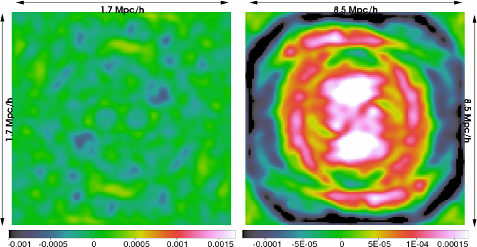
Figure 11: Plots similar to the plots in Fig. 10 except the the shear has been rotated by $45^{\circ}$ (B-mode) before transforming to the convergence fields. The thereby obtained convergence quantifies the statistical noise in the plots of Fig. 10.

One can relate the residual shear pattern in Fig. 9 to an excess in projected convergence (matter density) using the well known relation between convergence and cosmic shear in weak gravitational lensing (Bartelmann & Schneider 2001; Kaiser & Squires 1993):

$$\gamma_{\ell}=\frac{\ell_{1}^{2}-\ell_{2}^{2}+2{\rm i}\ell_{1}\ell_{2}}{\ell_{1}^{2}+\ell_{2}^{2}}\leavevmode\nobreak\ \kappa_{\ell}\;,$$ (29)

where $\gamma_{\ell}$ and $\kappa_{\ell}$ are the Fourier coefficients of the shear and convergence fields, respectively, on a grid and $\ell=(\ell_{1},\ell_{2})$ is a particular angular mode of the grid in Cartesian coordinates. We obtained the $\gamma_{\ell}$’s by employing Fast-Fourier-Transforms (and zero-padding to reduce undesired edge effects) after binning the residual shear patterns onto a $512\times 512$ grid. We assumed that the convergence is zero averaged over the box area which makes $\kappa_{\ell}=0$ for $\ell=0$. Fig. 10 shows the thereby computed maps. The plots were smoothed with a kernel of a size of a few pixels.

As a cross-check we also transformed the shear pattern produced by the $2^{\rm nd}$-order terms in $\tilde{\cal G}$ (Fig. 8) and found, as expected, that the corresponding convergence fields were just two identical radially symmetric “matter haloes” placed at the lens positions in the plot.

In the same way as in the previously discussed shear plots, parity invariance can also be checked in the convergence plots: quadrants I and IV (or II and III), mirrored about the $x$-axis, have to be statistically consistent. If we would like to enforce parity invariance, we could take the average of the two quadrants. Secondly, if one obtains the convergence field from the shear field via a Fourier transformation as described before, the convergence field will be a field of complex numbers. In the absence of any B-modes, however, the imaginary part will be zero or pure noise. Thus, the imaginary part of the convergence can be used to either check for residual B-modes or to estimate the noise level of the E-mode (real part).

This was done for Fig. 11. We found that the residual convergence for the small lens-lens separation is highly significant within the central region of Fig. 10, left panel, whereas the convergence in the right panel of Fig. 10 is noise dominated. This means we did not find any excess convergence beyond the noise level for the lens-lens pairs of large separation.

To sum up, one can see that closer lens pairs are embedded inside a common halo of excess matter, while the lenses with larger separation appear relatively disconnected; the convergence for the lenses of larger separation is lower by at least one order of magnitude and slips below noise level in our measurement. This result definitely deserves further investigation which we will do in a forthcoming paper.

5 Conclusions

We found a significant signal of GGGL in RCS – at least for the case for which we considered two lenses and one source. The signal is of an order of magnitude which is expected from a crude halo model-based prescription. This suggests a cosmological origin of the observed correlation.

In particular, our finding demonstrates that wide-field surveys of at least the size of RCS allow us to exploit GGGL. As can be seen in Fig. 4 (left), the remaining statistical uncertainties of the measurement are much smaller than the shift of the signal expected for different HODs of the adopted halo model. This means with GGGL we now have a new tool to strongly constrain galaxy HODs, and possibly even spatial distributions of galaxies inside haloes in general, which is a parameter in the framework of the halo model. As the wide-field shear surveys of the next generation will be substantially larger than RCS those constraints will become tighter. Further subdivisions of lens samples into different galaxy types and redshifts will therefore still give a reasonable signal-to-noise ratio.

Leaving the interpretation in the context of the halo model aside, the measurement of GGGL can be translated into a map of excess convergence around two galaxies of a certain mutual (projected) distance. For RCS, we demonstrated that there is a significant excess in convergence about two lenses if galaxies are as close as roughly $250\,h^{-1}\rm kpc$. Although the details need still to be worked out, this promises to be a novel way of studying the matter environment of groups of galaxies.