Superconducting-normal interface propagation speed in superconducting samples

Abstract

In this paper a new approach to obtain the interface propagation speed in superconductors by means of a variational method is introduced. The results of the approach proposed coincide with the numerical simulations. The hyperbolic differential equations are introduced as an extension of the model in order to take into account delay effects in the front propagation due to the pinning.

I Introduction

The study of interface propagation is one of the most fundamental problems in nonequilibrium physics. The understanding of the magnetic field penetration or expulsion in Superconducting samples has been a major challenge. An important problem to be solved is the determination of the speed at which the interface moves from a superconducting to a normal region.

In Ref.barto, , Di Bartolo and Dorsey have obtained the front speed by using heuristic methods such as Marginal stability hypothesis(MSH) and Reduction order.

In general, the nonlinear equations have been employed to model fronts propagation in different areas such as population growth and chemical reactions. Our start point is the nonlinear diffusion equations(ND) of the form $u_{t}=u_{xx}+f(u)$ obtained from the Ginzburg-Landau expressionsdorsey (GL). The GL comprise a coupled equations for the density of superconducting electrons and the local magnetic field.

Benguria and DepassierBengu1 ; Bengu2 ; Bengu3 have developed a variational speed selection method(BD) to compute the front speed in ND equations. In the BD method a trail function $g(x)$ is defined a priori and one may find accurate lower and upper bounds for the speed $c$. Only if the lower and the upper bounds coincide, then the value of $c$ can be determined without any uncertainty. To eliminate the ambiguity in the speed determination, Vincent and Fort in Ref.vincent, have proposed a more accurate approach based on the BD method. The approach assumes some approximative considerations from where the function $g(x)$ is determined.

The purpose of this paper is to develop further the insights into the front propagation afforded by the work in Ref.barto, . We aboard the determination of the propagation speed from a variational point of view. We use an alternative approach to the one developed by Vincent-Fortvincent .

In order to describe the evolution of the system between two homogeneous steady state, we assume a SC sample embedded in a stationary applied magnetic field equal to the critical $H=H_{c}$. The magnetic field is rapidly removed, so the unstable normal-superconducting planar interface propagates toward the normal phase so as to expel any trapped magnetic flux, leaving the sample in Meissner state. We have considered that the interface remains planar during all the process.

The existence of a delay time in the interface propagation systems is an important aspect that can be modeled by hyperbolic diffusion equations(HD) which generalize the ND. The HD has been recently applied in biophysics to model the spread of humansfort , bistable systemsmendez1 , forest firesmendez2 and in population dynamicsmendez3 . With the goal to take into account the delay effect on the interface propagation speeddorsey in superconductors, due to, for example, imperfections, vortex-vortex interactions, the presence of pinningaltshuler ; brandt , we have included the relaxation time $\tau$ for the front, and indee introduce the hyperbolic differential equations.

Traveling wave solutions. In this paper, we are interested in the one-dimensional time-dependent Ginzburg-Landau equations, which in dimensionless unitsdorsey are: $\partial_{t}f=(1/\kappa^{2})\,\,\partial^{2}_{x}f-q^{2}f+f-f^{3}$ and $\bar{\sigma}\partial_{t}q=\partial^{2}_{x}q-f^{2}q$.

Here, the quantity $f$ is the magnitude of the superconducting order parameter, $q$ is the gauge-invariant vector potential (such that $h=\partial_{t}q$ is the magnetic field), $\bar{\sigma}$ is the dimensionless normal state conductivity (the ratio of the order parameter diffusion constant to the magnetic field diffusion constant) and $\kappa$ is a parameter which determines the type of superconducting material; $\kappa<1/\sqrt{2}$ describes what are known as type-I superconductors, while $\kappa>1/\sqrt{2}$ describes what are known as type-II superconductors.

We are interested in finding traveling wave solutions for our model. We will search for steady traveling waves solutions for the GL equations of the form $f(x,t)=s(x-c\,t)$ and $q(x,t)=n(x-c\,t)$, where $z=x-c\,t$ with $c>0$. Then the equations become

$$\frac{1}{\kappa^{2}}\,\,s_{zz}+c\,s_{z}-n^{2}s+s-s^{3}=0,$$

$$n_{zz}+\bar{\sigma}c\,n_{z}-s^{2}n=0,$$ (1)

II Variational analysis

Vector potential $q=0$. In this section, we assume $q=0$ for the GL equations,

$$\partial_{t}f=\frac{1}{\kappa^{2}}\,\,\partial^{2}_{x}f+f-f^{3}.$$ (2)

Then, there exists a front $f=s(x-ct)$ joining $f=1$, the state corresponding to the whole superconducting phase to $f=0$ the state corresponding to the normal phase. Both states may be connected by a traveling front with speed $c$. The front satisfies the boundary conditions $\lim_{s\rightarrow-\infty}f=1,\lim_{s\rightarrow\infty}f=0$. Then Eq.(2) can be written as,

$$s_{zz}+c\,\kappa^{2}\,s_{z}+\mathfrak{F}_{k}(s)=0,$$ (3)

where $\mathfrak{F}_{k}=\kappa^{2}\,s(1-s^{2})$ and $\mathfrak{F}=(1/\kappa^{2})\mathfrak{F}_{k}$.

We define $p(s)=-ds/dz>0$ and $g$ such that $h=-dg/ds>0$. Taking into account $hp+(g\,\mathfrak{F}_{k}/p)\geq 2\,\sqrt{g\,h\,\mathfrak{F}_{k}}$ and following the BD methodBengu1 we arrive to

$$c\geq\,(2/\kappa)\,\int^{1}_{0}(g\,h\,\mathfrak{F})^{\frac{1}{2}}\,\,ds/\int^{1}_{0}g\,\,ds.$$ (4)

Now, the asymptotic speed of the front for sufficiently localized initial conditions may be determined in the limit $t\rightarrow\infty$. In the limit one has $s\rightarrow 1$ for $z\rightarrow-\infty$, and $s$ is a slowly varying function of $z$. Therefore one has $s_{zz}\ll\,s_{z}$, and from Eq.(3) we have that $\kappa^{2}\,c\,s_{z}+\kappa^{2}\,\mathfrak{F}(s)\simeq 0$ and $p\simeq\,-s_{z}\simeq\,\mathfrak{F}/c$.

Assuming $p=\mathfrak{F}(s)/\alpha>0$, where $\alpha$ is a positive constant to determine, we can write in general form the trial function as,

$$g(s)=\exp\,\left(-\,\alpha^{2}\int\,\mathfrak{F}^{-1}(s)\,ds\right).$$ (5)

Multiplying in both sides by the function $h$ in the expression $\mathfrak{F}_{k}g/p=hp$, we have that,

$$h\mathfrak{F}_{k}g=h^{2}p^{2}$$ (6)

By using Eq.(6), the relation $h\,\mathfrak{F}_{k}g=h^{2}\mathfrak{F}^{2}/\alpha^{2}$ is obtained. Then, the following relation is valid,

$$2\,\sqrt{h\,\mathfrak{F}_{k}\,g}=\,\frac{2}{\alpha}\,h\,\mathfrak{F}.$$ (7)

Substituting Eq.(7) in Eq.(4), the general expression for the speed is given by,

$$c\simeq\,max_{\alpha\in(0,1)}\left(\frac{2}{\alpha\,\kappa}\,\int^{1}_{0}\mathfrak{F}(s)\,h(s)\,\,ds/\int^{1}_{0}g(s)\,\,ds\right).$$ (8)

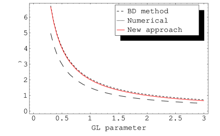
Figure 1: Illustration of the front speed obtained by different methods in the $q=0$ case versus the GL parameter.

Taking into account the form of $\mathfrak{F}$ and Eq.(5), the trial function can be written as

$$g(s)=\left[(s^{2}-1)/s^{2}\right]^{\alpha^{2}/2},$$ (9)

and the function $h(s)$,

$$h(s)=\alpha^{2}\,s^{-(1+\alpha^{2})}\,(1-s^{2})^{(\alpha^{2}-2)/2}.$$ (10)

The integrals in Eq.(8) are given by,

$$\int^{1}_{0}g(s)\,ds=\frac{1}{\sqrt{\pi}}\,\,\Gamma\left((1-\alpha^{2})/2\right)\,\Gamma\left(1+\alpha^{2}/2\right),$$ (11)

which is valid for $\alpha\geq 0$,

$$\int^{1}_{0}f(s)\,h(s)\,ds=\frac{1}{\sqrt{\pi}}\,[\,\Gamma\left((1-\alpha^{2})/2\right)$$ (12)

$$-2\,\Gamma\left((3-\alpha^{2})/2\right)]\,\Gamma\left(1+\alpha^{2}/2\right),$$

which is valid for $0<\alpha<1$.

Replacing Eqs.(11) and (12) in Eq.(8), we arrive to the speed for the front,

$$c\simeq\,max_{\alpha\in(0,1)}\,\,\frac{2}{\kappa\,\alpha}\,\left(1-\frac{2\,\Gamma\,\left[\frac{1}{2}\,(3-\alpha^{2})\right]}{\Gamma\,\left[\frac{1}{2}\,(1-\alpha^{2})\right]}\right).$$ (13)

Notice that for $\alpha=1$, we obtain the maximum for Eq.(13), $c=2/\kappa$ which is the result obtained by using the MSH method.

In Fig.1 the front speed versus the time delay is shown. The continuous line represents the results of the approach proposed in this paper following Eq.(13) and the numerical simulation by Eq.(2). The results coincides. Also, the dashed line represents the bound from the variational(BD) methodartorix .

Vector potential $q=1-f$. For a set of parametersbarto $\kappa=1/\sqrt{2}$ and $\bar{\sigma}=1/2$, we have that $s(z)+n(z)=1$, then Eq.(I) takes the form $s_{zz}+(c/2)\,s_{z}+\mathfrak{F}(s)=0$, where $\mathfrak{F}(s)=s^{2}(1-s)$ is the reaction term. Proceeding as in Eq.(5) we have that,

$$g(s)=\left[(1-s\right)/s]^{\alpha^{2}}\,\exp\left(\alpha^{2}/s\right),$$ (14)

and the velocity is given by,

$$c\simeq\,max_{\alpha\in\mathbb{D}}\left(\frac{2\,\sqrt{2}}{\alpha}\,\int^{1}_{0}\mathfrak{F}(s)\,h(s)\,\,ds/\int^{1}_{0}g(s)\,\,ds\right).$$ (15)

The interface speed is given by,

$$c\simeq\,max_{\alpha\in(0,1)}\left(2\,\sqrt{2}\,\alpha^{3}\,\frac{\Gamma(\alpha^{2})}{\Gamma(1+\alpha^{2})}\right),$$ (16)

for $\alpha=1/2$ we obtain the maximum for Eq.(16), then $c=\sqrt{2}$ which is the result obtained by using the MSH method.

III Front flux expulsion with delay

It is well known the existence of pinning produces a delay timealtshuler in the magnetic field penetration o expulsion. This can be taken into account by resorting to hyperbolic differential equations seen in Section I, which generalize the parabolic equation. The aim of this section is to study of the interface speed problem in superconducting samples by means of the HD equations, which can be written as

$$\tau\,\frac{\partial^{2}\,u}{\partial\,t^{2}}+\frac{\partial\,u}{\partial\,t}=\,\frac{\partial^{2}\,u}{\partial\,x^{2}}+f(u)+\tau\,\frac{\partial\,f(u)}{\partial\,t},$$ (17)

In the absence of a delay time $(\tau=0)$, this reduces to the classical equation $u_{t}=u_{xx}+f(u)$.

Vector potential $q=0$. Taking into account the Eqs.(2) and (17) we can write the following expression,

$$\kappa^{2}\,\tau\,\frac{\partial^{2}\,f}{\partial\,t^{2}}+\kappa^{2}\,\frac{\partial\,f}{\partial\,t}=\frac{\partial^{2}\,f}{\partial\,x^{2}}+\kappa^{2}\,\mathfrak{F}+\kappa^{2}\,\tau\,\frac{\partial\,\mathfrak{F}}{\partial\,t},$$ (18)

where $\mathfrak{F}=s(1-s^{2})$.

It has been provedmendez1 ; mendez2 ; mendez3 that Eq.(17) has traveling wave fronts with profile $s(x-ct)$ and moving with speed $c>0$. Then we can write Eq.(18) as follows,

$$(1-a\,c^{2})\,s_{zz}+c\,[\kappa^{2}-a\,\mathfrak{F}^{\prime}(s)]\,s_{z}+\mathfrak{F}_{k}(s)=0,$$ (19)

where $z=x-ct$, $a=\kappa^{2}\,\tau$, $\mathfrak{F}_{k}=\kappa^{2}\,\mathfrak{F}$, and with boundary conditions $lim_{z\rightarrow\infty}s=0$, $lim_{z\rightarrow-\infty}s=1$, and $s_{z}<0$ in $(0,1)$; $s_{z}$ vanishes for $z\rightarrow\pm\infty$.

We define $p(s)=-ds/dz>0$ and $g$ such that $h=-dg/ds>0$. Taking into account $(1-a\,c^{2})hp+(g\mathfrak{F}_{k}/p)\geq 2\sqrt{1-ac^{2}}\,\sqrt{g\,h\,\mathfrak{F}_{k}}$ and following the BD method we arrive to

$$\frac{c}{\sqrt{1-a\,c^{2}}}\geq\,2\,\kappa\,\frac{\int^{1}_{0}(g\,h\,\mathfrak{F})^{1/2}\,ds}{\int^{1}_{0}g(\,\kappa^{2}-a\,\mathfrak{F}^{\prime})\,ds}.$$ (20)

In order to obtain the trial function $g(s)$, we take in consideration that in the lim $s\rightarrow 1$ we get

$$-c\,[\kappa^{2}-a\,\mathfrak{F}^{\prime}(s)]\,p\,+\,\mathfrak{F}_{\kappa}(s)\simeq 0,$$ (21)

since $s_{zz}\ll s_{z}$. Then, we write an expression for $p$ in terms of $\mathfrak{F}$,

$$p=\mathfrak{F}_{\kappa}/\alpha\,[\kappa^{2}-a\,\mathfrak{F}^{\prime}(s)].$$ (22)

The expression for the speed is given by,

$$\frac{c}{1-a\,c^{2}}\simeq max_{\alpha\in(0,1)}\,\frac{2\,\kappa^{2}}{\alpha}\,\frac{\int^{1}_{0}\left[h\,\mathfrak{F}\,/(\,\kappa^{2}-a\,\mathfrak{F}^{\prime})\right]\,ds}{\int^{1}_{0}g(\,\kappa^{2}-a\,\mathfrak{F}^{\prime})\,ds},$$ (23)

where the integrals can be only solved by numerical methods. Taking into account Eq.(22) and the expressionmendez1 $(1-ac^{2})hp=\mathfrak{F}_{\kappa}g/p$, we have obtained the relation for the trial function,

$$g=\exp\left[-\frac{\alpha^{2}}{(1-ac^{2})}\int\,\frac{(\kappa^{2}-a\,\mathfrak{F}^{\prime})^{2}}{\mathfrak{F}_{\kappa}}\,ds\right].$$ (24)

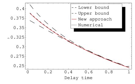
Figure 2: Time-delayed interface propagation speed for the case of $q=0$ versus the time delay $\tau$.

from where we have for our case,

$$g=\exp\left[\frac{\alpha^{2}}{2\kappa^{2}(1-ac^{2})}\left((3as)^{2}+\lg\left[\frac{(s^{2}-1)^{(2a+\kappa^{2})^{2}}}{s^{2(a-\kappa^{2})^{2}}}\right]\right)\right],$$ (25)

and for $h$,

$$h(s,\alpha,a)=\frac{\alpha^{2}\,\left(\kappa^{2}+a(3s^{2}-1)\right)^{2}}{\kappa^{2}\,s(s^{2}-1)\,(a\,c^{2}-1)}\,\,g(s,\alpha,\kappa)$$ (26)

In Fig.2 the front speed versus the time delay is shown. The continuous line represents the result of the approach proposed in this paper following Eq.(23) which coincides with the numerical simulation done using Eq.(18). Also, we have represented the lower and upper bounds from the variational(BD) methodartorix .

Vector potential $q=1-f$. Taking into account the Eqs.(17) and (18) we can write the following expression,

$$\frac{\tau}{2}\,\frac{\partial^{2}\,f}{\partial\,t^{2}}+\frac{1}{2}\,\frac{\partial\,f}{\partial\,t}=\frac{\partial^{2}\,f}{\partial\,x^{2}}+\frac{1}{2}\,\mathfrak{F}+\frac{\tau}{2}\,\frac{\partial\,\mathfrak{F}}{\partial\,t},$$ (27)

where $\mathfrak{F}=s^{2}(1-s)$.

Then we can write Eq.(27) as follows,

$$(1-a\,c^{2})\,s_{zz}+c\,[\kappa^{2}-a\,\mathfrak{F}^{\prime}(s)]\,s_{z}+\mathfrak{F}_{k}(s)=0,$$ (28)

where we have assumed $\mathfrak{F}_{k}=(1/2)\mathfrak{F}$ and $a=\tau/2$.

The expression for the velocity is given by

$$\frac{c}{\sqrt{1-ac^{2}}}\geq\,2\,\sqrt{2}\,\frac{\int^{1}_{0}(g\,h\,\mathfrak{F})^{1/2}\,ds}{\int^{1}_{0}g(1-2\,a\,\mathfrak{F}^{\prime})\,ds}.$$ (29)

In order to obtain an expression for the trial function $g(s)$, we take in consideration that in the lim $s\rightarrow 1$ we get

$$-c\,[(1/2)-a\,\mathfrak{F}^{\prime}(s)]\,p\,+\,\mathfrak{F}_{\kappa}(s)\simeq 0,$$ (30)

since $s_{zz}\ll s_{z}$. Then, we write an expression for $p$ in terms of $\mathfrak{F}$,

$$p=\mathfrak{F}_{\kappa}/\alpha\,[(1/2)-a\,\mathfrak{F}^{\prime}].$$ (31)

The expression for the speed is given by,

$$\frac{c}{1-a\,c^{2}}\simeq max_{\alpha\in(0,1)}\,\frac{2\,\kappa^{2}}{\alpha}\,\frac{\int^{1}_{0}\left[h\,\mathfrak{F}\,/(\,(1/2)-a\,\mathfrak{F}^{\prime})\right]\,ds}{\int^{1}_{0}g(\,(1/2)-a\,\mathfrak{F}^{\prime})\,ds}.$$ (32)

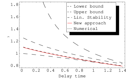
Figure 3: Time-delayed interface propagation speed for $q=1-f$ versus the time delay.

Taking into account Eq.(31) and the expressionmendez1 $(1-ac^{2})hp=\mathfrak{F}_{\kappa}g/p$, we have obtained the relation for the trial function,

$$g=\exp\left[-\frac{\alpha^{2}}{(1-ac^{2})}\int\,\frac{((1/2)-a\,\mathfrak{F}^{\prime})^{2}}{\mathfrak{F}_{\kappa}}\,ds\right].$$ (33)

from where we have for our case,

$$g(s,\alpha,a)\,=\,\exp\left[\frac{\alpha^{2}}{4\,s\,(1-ac^{2})}\left(g_{1}+g_{2}\right)\right],$$ (34)

where $g_{1}=1+24\,a^{2}\,s^{2}(3s-2)$, and $g_{2}=\lg\,(s-1)^{s\,(4a+1)^{2}}\,s^{s\,(16\,a-1)}$,

$$h(s,\alpha,a)=\frac{\alpha^{2}\,\left[1+4\,a\,s(3s-2)\right]}{4\,s^{2}(1-s)\,(1-a\,c^{2})}\>\,g(s,\alpha,a)$$ (35)

The integrals in Eq.(32) can be only solved by numerical methods.

In Fig.3 the front speed versus the time delay is shown. The continuous line represents the results based on the approach proposed in this paper following Eq.(32) which coincides with the numerical simulation done using Eq.(27). Also, we have represented the lower and upper bounds from the variational(BD) methodartorix .

Conclusion. We have computed for the Ginzburg-Landau equations in the form of parabolic and hyperbolic equations the superconducting-normal interface propagation speed by a new approach. This approach is based in the method proposed by Vincent and Fort in Ref.vincent, . We have obtained the expressions for the trial function $g$ in each case developed. The results of our methodology coincide with the numerical results for the examples analyzed.

References

• (1) J.Bartolo and A.Dorsey, Phys.Rev.Lett. 77, 4442(1996)
• (2) A.T. Dorsey, Ann. Phys. (N.Y.) 233, 248(1994)
• (3) R.Benguria and M.Depassier,Phys.Rev.Lett.73,2272(1994)
• (4) R.Benguria and M.Depassier, Phys.Rev.E. 57, 6493(1998)
• (5) R.Benguria and M.Depassier, Phys.Rev.E. 52, 3258(1995)
• (6) V. Mendez and J. Fort, Phys.Rev.E. 64, 011105(1997)
• (7) J. Fort and V. Mendez, Phys. Rev. Lett. 82, 867(1999)
• (8) V. Mendez and A. Compte, Physica A 260, 90(1998)
• (9) V. Mendez and J.E. Lebot, Phys. Rev. E. 56, 6557(1997)
• (10) V. Mendez and J. Camacho, Phys. Rev. E. 55, 6476(1997)
• (11) E.Altshuler and T.Johansen, Rev.Mod.Phys.76, 471(2004)
• (12) E.H. Brandt, Rep. Prog. Phys. 58, 1465(2002)
• (13) A. de la Cruz de Ona, Sumitted to Phys. Rev. B(2007), eprint arXiv: 0705.0896