The nonlinear evolution of instabilities driven by magnetic buoyancy: A new mechanism for the formation of coherent magnetic structures

Abstract

Motivated by the problem of the formation of active regions from a deep-seated solar magnetic field, we consider the nonlinear three-dimensional evolution of magnetic buoyancy instabilities resulting from a smoothly stratified horizontal magnetic field. By exploring the case for which the instability is continuously driven we have identified a new mechanism for the formation of concentrations of magnetic flux.

1. Introduction

Solar active regions are the surface manifestations of a deep-seated, predominantly toroidal magnetic field. Although it is generally agreed that the solar magnetic field is maintained by some sort of hydromagnetic dynamo, the mechanism by which this is effected is far from understood. Consequently, the strength, structure, and location of the interior magnetic field are similarly unknown. However, most recent solar dynamo models, despite their significant differences in other respects, postulate that the tachocline, the thin layer of strong velocity shear located at the base of the convection zone, plays an important role in the generation of toroidal field by the shearing of a weaker poloidal component (see, e.g., the review by Tobias & Weiss, 2007). Given this premise, it is important to address the nature of the initial escape of the magnetic field from the tachocline, its subsequent ascent through the convection zone, and its eventual emergence at the photosphere.

Owing to the vast range of scales across the convection zone, it is impossible to model realistically all of these stages in one calculation. Here we concentrate solely on the instability of a layer of magnetic field, with the aim of clarifying the physics of the formation of coherent magnetic structures from a much larger scale field.

A vertically stratified, horizontal magnetic field can be unstable to magnetic buoyancy instability provided that the field decreases sufficiently rapidly with height. It is important to note the non-trivial distinction between instability to two-dimensional modes in which the field lines remain straight (interchange modes) and instability to fully three-dimensional modes. The former are essentially destabilized by a decrease with height of $B/\rho$ (where $B$ is the magnetic field strength and $\rho$ the density), the latter simply by a decrease with height of $B$. The physics underlying this difference is elucidated in Hughes & Cattaneo (1987).

The linear theory of magnetic buoyancy instabilities has been intensively studied over a number of years (e.g. Newcomb, 1961; Parker, 1966; Gilman, 1970; Acheson, 1978). The nonlinear development of the instability, particularly with respect to a deep-seated solar field, has, inevitably, received less attention. Cattaneo & Hughes (1988) investigated the nonlinear evolution of interchange modes resulting from a slab of uniform horizontal magnetic field embedded in a convectively stable and otherwise field-free atmosphere. Here the instability is driven by a density jump at the upper interface of the magnetic slab — an extreme form of magnetic buoyancy instability. This interfacial instability generates a strong shear flow that leads, by a secondary Kelvin-Helmholtz instability, to the formation of strong vortices. The subsequent nonlinear evolution is then governed by pairwise vortex interactions, which can even act so as to drag down pockets of strong magnetic field. The three-dimensional instability and nonlinear evolution of the same basic state was examined by Matthews et al. (1995) and Wissink et al. (2000). The initial evolution again takes the form of interchange modes, leading to the formation of vortex tubes. However, neighbouring vortex tubes of opposite sign are unstable to a longitudinal instability (Crow, 1970); this in turn causes the magnetic field to adopt an arched structure. By contrast, Fan (2001) investigated the nonlinear evolution of a smoothly varying magnetic field, with a profile chosen such that the initial state is unstable to three-dimensional modes, but stable to interchange modes. She shows the formation of arched magnetic structures, which maintain a reasonable degree of coherence as they rise. A recent review of the implications of magnetic buoyancy instabilities for the solar tachocline is given by Hughes (2007). Related simulations of magnetic buoyancy in sub-surface regions have also been performed (e.g. Archontis et al., 2004; Isobe et al., 2005).

Inspection of active regions on the solar surface suggests the emergence through the photosphere of a buckled, toroidal magnetic field. However, very little is known about the structure, strength and orientation of the sub-surface field. For example, which properties of the observed surface field result from the initial instability and which result from later interactions in the convection zone? Our aim in this Letter is to seek further understanding of the instability by examining the nonlinear evolution from a very simple equilibrium state. We consider an atmosphere that is in both magnetohydrostatic and thermal equilibrium and that has a linear magnetic field profile. We concentrate on modes that are intrinsically three-dimensional; i.e. the field gradients considered are such that the basic state is unstable to three-dimensional modes but stable to interchanges.

Furthermore, we impose boundary conditions such that the source of the instability is maintained for all times, thus allowing us to consider the long-term evolution. This is an important difference from the earlier works cited above, all of which consider “run-down” experiments, in which the potential energy stored in the initial field configuration is rapidly converted into kinetic energy and which is then slowly dissipated.

We consider four cases, characterised by two different field strengths and two different choices of initial conditions. We have identified a completely new mechanism for the formation of flux concentrations; this is of potential significance in the solar context in which the formation of localised regions of strong field from a weaker larger scale field is a crucial component of the flux emergence process.

Figure 1.— Model with $\alpha=\frac{1}{4}$ and eigenfunction perturbation. (a) Evolution of the kinetic energy density. (b) Horizontal average of the magnetic field $B_{x}$ vs. depth, initially (dotted line), at $t\approx 50$ (dashed line), and in the final steady state (solid line).

2. Mathematical formulation and parameters

We consider a Cartesian layer of perfect gas governed by the equations of three-dimensional compressible MHD. The dimensionless representation of these equations is obtained by scaling lengths with the layer depth, time with the isothermal sound crossing time at the top surface ($z=0$), and temperature, density, and magnetic field with their respective values at the top surface. The physical properties of the fluid are entirely determined by four dimensionless numbers: the Prandtl number $P_{r}$, the ratio of viscous to thermal diffusivity; $\zeta$, the ratio of magnetic to thermal diffusivity; $\gamma$, the ratio of specific heats; and $C_{k}$, the nondimensional thermal conductivity.

The basic state that we consider is an exact equilibrium, dependent only on depth $z$, with a unidirectional horizontal magnetic field $B_{x}(z)=1+z/H_{b}$. The density and temperature are determined from solution of the magnetohydrostatic equations. In the absence of a magnetic field, the atmosphere takes the form of a plane polytrope, with polytropic index $m$ and constant temperature gradient $\theta$. The strength of the magnetic field is changed by varying $\alpha=2/\beta\propto B^{2}$, where the plasma-$\beta$ is the ratio of the thermal to the magnetic pressure. A more detailed description of the governing equations and parameters is contained in Tobias et al. (1998).

We consider perturbations to this basic state, subject to the following boundary conditions: all variables are taken to be periodic in both horizontal directions; the top and bottom boundaries are stress-free, impermeable, and isothermal. For the magnetic field we choose to maintain a fixed gradient of $B_{x}$ ($\partial B_{x}/\partial z=1/H_{b}$) at $z=0,1$, together with $\partial B_{y}/\partial z=0$ and $B_{z}=0$. Our aim in this Letter is to examine the nonlinear development of modes that are intrinsically three-dimensional. By an extensive linear analysis we have identified the regions in parameter space where three-dimensional modes ($k_{x}\neq 0$, $k_{y}\neq 0$) are unstable but interchange modes ($k_{x}=0$) are stable. In the next section we discuss the nonlinear evolution resulting from two choices of parameters and two different types of perturbation to the basic state.

3. Nonlinear evolution of three-dimensional modes

The nonlinear evolution of three-dimensional magnetic buoyancy instabilities is studied by solving numerically the equations of compressible MHD with a modified version of the hybrid finite-difference-pseudospectral parallel code used by Brummell et al. (1996) (hydrodynamic) and Tobias et al. (1998) (MHD). We consider the evolution from two basic states, distinguished by the value of the field strength; the other parameters are held fixed at $P_{r}=\zeta=2\times 10^{-2}$, $C_{k}=2.5\times 10^{-2}$, $\theta=2$, $m=1.6$, $H_{b}=1$, and $\gamma=5/3$. Furthermore, we consider two different perturbations to each basic state: one consisting of the most unstable eigenfunction, the other of random noise. In each case, the horizontal dimensions of the Cartesian computational box are determined by the wavenumbers $k_{x}$ and $k_{y}$ of the most unstable mode such that one wavelength fits in the $x$-direction, along the initial magnetic field, and four wavelengths fit transverse to the initial field, in the $y$-direction.

3.1. Evolution to a Steady State

Here we consider a basic state with $\alpha=1/4$ perturbed by the most unstable eigenfunction, namely, that with growth rate $\sigma=0.16$ and with wavenumbers $k_{x}=0.87$ and $k_{y}=8.38$ (hence, the dimensions of the computational domain are $L_{x}=7.24$ and $L_{y}=3$). The evolution is essentially linear up to time $t\approx 21$. For $21\lesssim t\lesssim 37$ the kinetic energy continues to grow (see Fig. 1a). During this stage, broad upflows carry strong magnetic fields from the bottom of the layer, while narrow plumes pull down weaker field, leading to the formation of arched structures, as shown in Figure 2. Figure 1b shows the mean result of this nonlinear evolution, with a significant reduction of the gradient of the horizontally averaged magnetic field $B_{x}$. Initially constant throughout the layer (dotted line), the vertical gradient of $B_{x}$ becomes nearly zero in a large fraction of the domain at $t\approx 50$ (dashed line). The nonlinear reorganization has therefore acted to remove the driving mechanism of the instability. There is an obvious analogy with thermal convection, in which saturation is achieved by a nonlinear reorganization leading to an adiabatic core with thin thermal boundary layers.

The arched configuration shown in Figure 2 is however transient; following this initial nonlinear reorganization the system relaxes to a state with weak flows and a magnetic field profile that is close to critical. As can be seen from Figure 1b, the field gradient in the final state is reduced everywhere in the layer compared with its initial value. This subsequent evolution is permitted by the choice of boundary conditions, in which the gradient of $B_{x}$ (but not the field itself) is fixed at the boundaries.

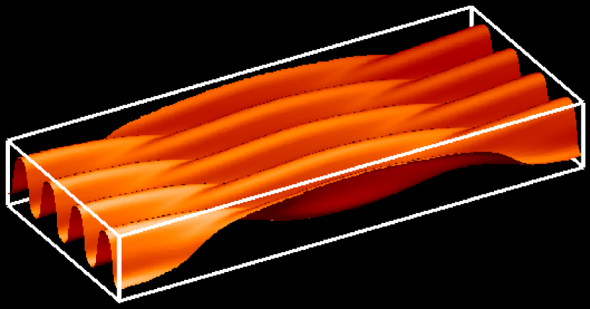
Figure 2.— Isosurface of magnetic energy $(B^{2}/2=1)$ at $t\approx 45$ for the same model as in Fig. 1.

3.2. Evolution to Time-dependent Concentrated Flux States

First we consider the evolution from the same basic state as in §3.1 (i.e. with $\alpha=1/4$), but with the perturbation taking the form of small-amplitude random noise. As shown in Figure 3a, the linear evolution (up to $t\approx 36$) and the initial nonlinear phase, as measured by the temporal evolution of gross properties such as kinetic energy, are similar to those portrayed in Figure 1a . The first nonlinear reorganization again leads to the formation of arched structures, as shown in Figure 4, although, as a result of the initial conditions, these are less regular than those of Figure 2. Crucially, these irregularities play a significant role in modifying the subsequent behaviour. From $100\lesssim t\lesssim 450$ the kinetic energy increases monotonically until the onset of a secondary oscillatory instability. From $t\approx 1200$ the system evolves on two disparate timescales: a short cycle with period $\approx 7$ modulated on larger timescales $250\lesssim t_{\text{mod}}\lesssim 300$.

The underlying mechanism of the short period oscillations can be understood by inspection of Figure 3b, which shows the temporal evolution for fixed values of $x$ and $z$ of the magnetic energy, the transverse horizontal velocity $v$, and the vertical velocity $w$. The left panel shows the periodic formation of a concentration of magnetic energy, which drifts slowly with velocity $0.03$. The central and right panels indicate that the concentrations of magnetic energy result from convergent downflows associated with rolls in the $yz$-plane. The magnetic flux becomes concentrated between the two counter-rotating rolls; it thus becomes buoyant and rises rapidly. This drives a countercell, which diverges at the flux concentration and thereby destroys it. After some reorganization, the initial cellular flow is reestablished but displaced relative to its initial position. Reformed downflows again lead to a concentration of flux and the entire process is repeated.

Next we examine the evolution from an equilibrium with a stronger field ($\alpha=1$). For this case the evolution is qualitatively similar regardless of the nature of the initial perturbation; here we shall describe the case in which the perturbation takes the form of random noise. The most unstable mode has wavenumbers $k_{x}=0.86$ and $k_{y}=9.75$, and growth rate $\sigma=0.45$. Figure 5a shows that the temporal evolution is broadly similar to that of the weaker field case portrayed in Figure 3a. The secondary instability is evident, leading to a modulated periodic state. The increase in initial field strength leads, as expected, to a more vigorous instability (higher growth rate and increased saturation level) and to a shorter period oscillation of the nonlinear state. As in the example above, flux concentration occurs via converging downflows. The peak field in the flux concentrations is significantly stronger than the average initial field. In this case, as can be seen in Figure 6, the flux concentrations are never completely dispersed, although their strength varies as they propagate. This (modulated) travelling wave behaviour for the field and flows can be clearly seen in Figure 5b.

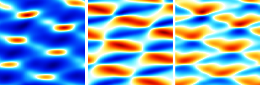
Figure 3.— Model with $\alpha=\frac{1}{4}$ and random perturbation. (a) Evolution of the kinetic energy density. (b) Space-time plots, with $y$ horizontal and $t$ vertical, of magnetic energy $(1.17\lesssim B^{2}/2\lesssim 1.78)$, $|v|\lesssim 0.05$, and $|w|\lesssim 0.06$; $1863\lesssim t\lesssim 1913$; $z\approx 0.7$.

4. Discussion

In this Letter we have identified a new, inherently nonlinear, mechanism for the formation of coherent magnetic structures from a layer of weaker magnetic field. The initial development of the magnetic buoyancy instability drives flows that act so as to form isolated concentrations of magnetic flux. This nonlinear state persists because the instability is continually driven from the boundaries and saturation of the instability occurs via the net redistribution of flux so as to remove average magnetic field gradients from the interior of the computational domain. An intriguing feature of the flux concentrations is that, once established, they travel — taking the form of a modulated wave.

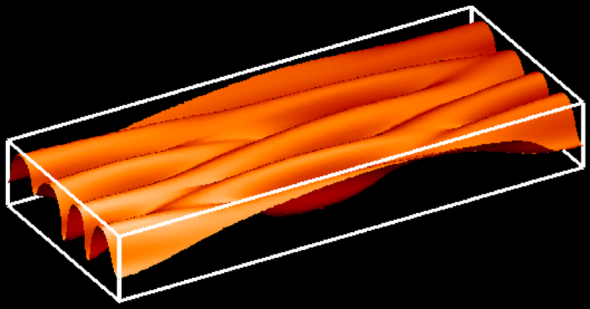
Figure 4.— Isosurface of magnetic energy $(B^{2}/2=1)$ at $t\approx 74$ for the same model as in Fig. 3.

The processes in the deep interior of the Sun that lead to the formation of active regions are still poorly understood. Even the most optimistic estimates from dynamo theory suggest that an upper bound for the large-scale dynamo-generated field is of the order of $10^{4}$ G (see, e.g. Ossendrijver, 2003). The energy of such a field is small, however, in comparison with that of the strong downflows in the convection zone and, such a field might be expected to be pinned down by the convection (see, e.g. Tobias et al., 1998). Clearly, therefore, some process must be acting so as to create strong localised field structures from the dynamo field that are capable of traversing the convection zone in order to form active regions. Our calculations, although idealized, suggest a new mechanism that may play a key role in this process.

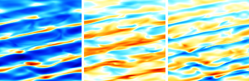
Figure 5.— Same as Fig. 3, but with $\alpha=1$. In panel b $0.65\lesssim B^{2}/2\lesssim 2.27$, $|v|\lesssim 0.51$, $|w|\lesssim 0.56$; $153\lesssim t\lesssim 200$; and $z\approx 0.5$.

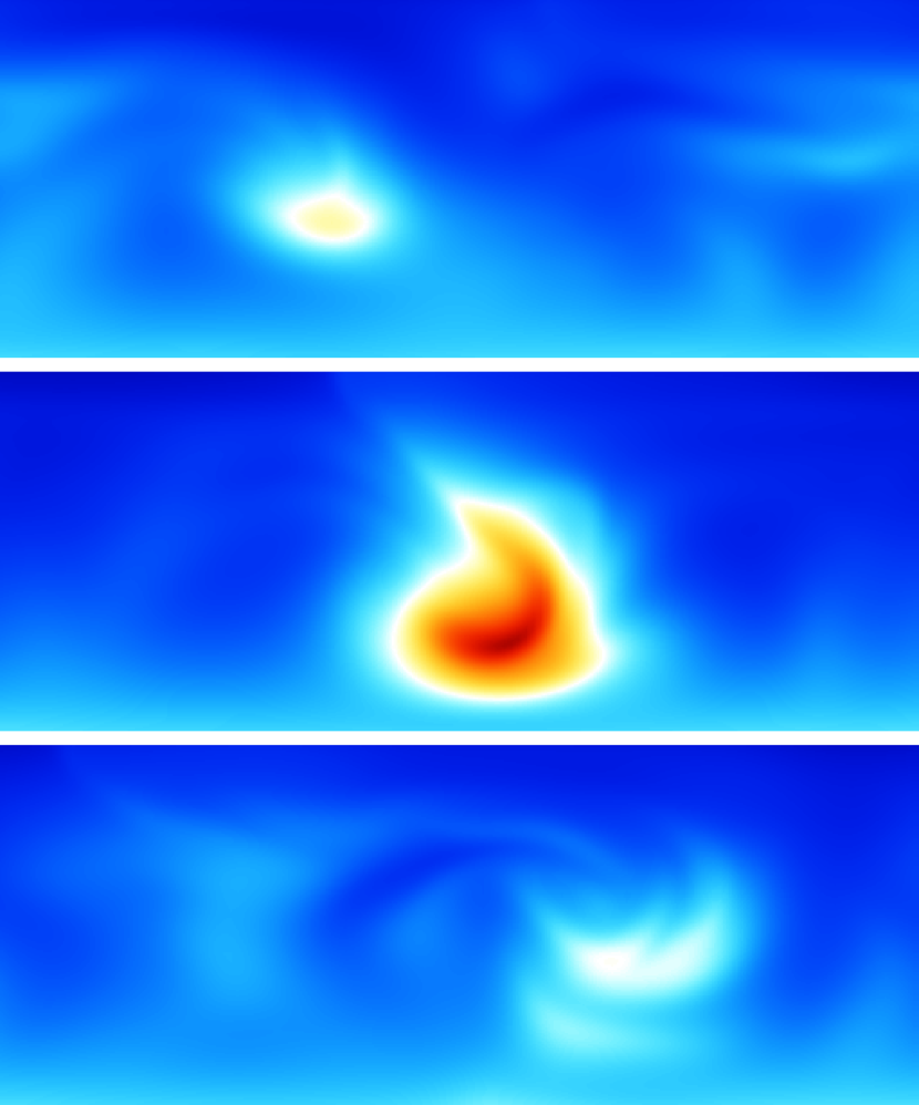
Figure 6.— Slices in the $yz$-plane of magnetic energy at times $t\approx 152.9$, $154.7$, $156.5$. The peak magnetic energy $\approx 3$.

We conclude by noting that the discovery of the mechanism arose from considering a system where the instability is continually driven, in contrast to nearly all previous studies in which the initial magnetic buoyancy instability was investigated by means of run-down calculations. Both types of experiment may be of importance for understanding the dynamics of the solar interior. The magnetic buoyancy instability is a fast process that might be captured by run-down calculations (which usually lead to the formation of arched structures). On the other hand, the replenishment of toroidal field by the dynamo should lead to a continual source of instability of field at the base of the solar convection zone.

References

- Acheson (1978) Acheson, D. J. 1978, Phil. Trans. R. Soc. London A, 289, 459
- Archontis et al. (2004) Archontis, V., Moreno-Insertis, F., Galsgaard, K., Hood, A., & O’Shea, E. 2004, A&A, 426, 1047
- Brummell et al. (1996) Brummell, N. H., Hurlburt, N. E., & Toomre, J. 1996, ApJ, 473, 494
- Cattaneo & Hughes (1988) Cattaneo, F. & Hughes, D. W. 1988, J. Fluid Mech., 196, 323
- Crow (1970) Crow, S. C. 1970, AIAA, 8, 2172
- Fan (2001) Fan, Y. 2001, ApJ, 546, 509
- Gilman (1970) Gilman, P. A. 1970, ApJ, 162, 1019
- Hughes (2007) Hughes, D. W. 2007, in The Solar Tachocline, ed. D. W. Hughes, R. Rosner, & N. O. Weiss (Cambridge: Cambridge Univ. Press), 275
- Hughes & Cattaneo (1987) Hughes, D. W. & Cattaneo, F. 1987, Geophys. Astrophys. Fluid Dyn., 39, 65
- Isobe et al. (2005) Isobe, H., Miyagoshi, T., Shibata, K., & Yokoyama, T. 2005, Nature, 434, 478
- Matthews et al. (1995) Matthews, P. C., Hughes, D. W., & Proctor, M. R. E. 1995, ApJ, 448, 938
- Newcomb (1961) Newcomb, W., A. 1961, Phys. Fluids, 4, 391
- Ossendrijver (2003) Ossendrijver, M. 2003, A&A Rev., 11, 287
- Parker (1966) Parker, E. N. 1966, ApJ, 145, 811
- Tobias et al. (1998) Tobias, S. M., Brummell, N. H., Clune, T. L., & Toomre, J. 1998, ApJ, 502, L177
- Tobias & Weiss (2007) Tobias, S. M. & Weiss, N. O. 2007, in The Solar Tachocline, ed. D. W. Hughes, R. Rosner, & N. O. Weiss (Cambridge: Cambridge Univ. Press), 319
- Wissink et al. (2000) Wissink, J. G., Hughes, D. W., Matthews, P. C., & Proctor, M. R. E. 2000, MNRAS, 318, 501