Driving-dependent damping of Rabi oscillations in two-level semiconductor systems

Abstract

We propose a mechanism to explain the nature of the damping of Rabi oscillations with increasing driving-pulse area in localized semiconductor systems, and have suggested a general approach which describes a coherently driven two-level system interacting with a dephasing reservoir. Present calculations show that the non-Markovian character of the reservoir leads to the dependence of the dephasing rate on the driving-field intensity, as observed experimentally. Moreover, we have shown that the damping of Rabi oscillations might occur as a result of different dephasing mechanisms for both stationary and non-stationary effects due to coupling to the environment. Present calculated results are found in quite good agreement with available experimental measurements.

Localized semiconductor systems exhibiting few discrete energy levels (”artificial atoms”), such as specially selected donor impurities and quantum dots (QDs), are prospective candidates to play the role of basic building blocks for quantum information processing. In particular, a two-level semiconductor system may exhibit Rabi oscillations (ROs) of its population when coupled to a driving field, so that it may be coherently controlled experiment ; exper ; no-biexciton ; int_indep ; traps . There are a number of dephasing mechanisms for localized semiconductor systems, some of which are essentially non-Markovian so that one needs to take into account memory effects as well as the back-action of a dissipative reservoir on the radiating system. For example, a dephasing caused by spin-spin coupling between neighboring QDs or carriers captured in traps in the vicinity of a QD was shown to lead to non-Markovian dynamics apn-works ; spin . Such reservoirs have correlation times comparable with the typical decoherence time of the dephasing system. Also, the dephasing due to coupling with phonons was shown to lead to non-Markovian features in the dynamics of a two-level systems (TLS) phonon . Carriers and excitons in localized semiconductor systems may be coupled not only to localized neighboring states, but also to delocalized ones deloc . This diversity of dissipation channels has led to a number of novel features in such systems’ dynamics. In the present work we focus our attention on one peculiar phenomenon which has caused and is still causing much controversy, namely, the damping of ROs due to the increase of the driving-pulse area which is an observed feature of coherently excited localized semiconductor systems experiment ; exper ; no-biexciton ; int_indep ; traps . A number of mutually contradicting explanations was suggested for it. One of these is that such a dephasing is due to the system’s interaction with a non-Markovian reservoir of phonons phonon . However, the dephasing process takes place even when the coupling with phonons is negligible no-biexciton . Driving-dependent damping of ROs was proposed to occur as a consequence of excitations of bi-excitons in the QD biexciton , although damped ROs are also observed when there is no possibility for the bi-exciton excitation no-biexciton . Recently, it was demonstrated that the experimentally observed exper intensity-dependent damping of ROs can be reproduced by introducing into the standard Bloch equations a dephasing rate dependent on the driving-field intensity oliveira . On the other hand, although there is an experimental confirmation of a driving dependence of the dephasing rate no-biexciton , an intensity-independent dephasing rate has also been measured int_indep .

Based on this controverted scenario, in the present work we propose to shed some light on this matter by studying a simple TLS excited by a classical coherent field and coupled to a general dephasing reservoir. Within a quite general and straightforward approach, we demonstrate that a driving-field dependent damping of ROs stems from various relaxation mechanisms entering into play in different experimental situations. Furthermore, we show that driving-dependent damping may occur whether the reservoir is influenced or not by the driving field. To keep it simple, and to focus only on features which give rise to the phenomenon in question, we assume no population damping of the TLS. This also corresponds to the real experimental situation with driving by short laser pulses, so that the population damping is negligibly slow on the time-scale of the system’s dynamics exper . In the frame rotating with the driving-field frequency, $\omega_{L}$, working within the interaction picture with respect to the reservoir variables and using the rotating-wave approximation (RWA), we describe our problem with the following standard effective Hamiltonian,

$$H_{tot}(t)=H_{0}(t)+\hbar\sigma^{+}\sigma^{-}{\bf R}(t),$$ (1)

where the undamped system’s Hamiltonian is given by

$$H_{0}(t)=\hbar\Delta\sigma^{+}\sigma^{-}+\hbar[\Omega(t)\sigma^{+}+\Omega^{*}(t)\sigma^{-}].$$ (2)

Here $\sigma^{\pm}=|\pm\rangle\langle\mp|$ are the system’s raising and lowering operators, the kets $|\pm\rangle$ correspond to the excited and ground states of the TLS, respectively, $\Delta=\omega_{0}-\omega_{L}$ is the detuning of the driving-laser frequency $\omega_{L}$ from the resonance frequency $\omega_{0}$ of the TLS transition, with the possible addition of a frequency-shift term due to the interaction with the dephasing reservoir. The reservoir is described by the operator ${\bf R}(t)$, which might also depend on classical stochastic variables (describing, for example, different realizations of the reservoir in each run of an experiment apn-works ), whereas $\Omega(t)$ describes the shape of the driving pulse.

Let us now assume that the reservoir correlation function $\langle{\bf R}(t){\bf R}(\tau)\rangle$ satisfies the following general requirements: $\langle{\bf R}(t){\bf R}(\tau)\rangle\rightarrow 0$, when $t,\tau\rightarrow\infty$, and $|t-\tau|\rightarrow\infty$. If the coupling of the reservoir to the TLS is weak, and the reservoir correlation function decays with $t,\tau\rightarrow\infty$, and also with $|t-\tau|\rightarrow\infty$ much faster than the typical time-scale of the system’s evolution, it is possible to obtain a time-local master equation apn-works ; tlmast for the problem described by the Hamiltonian (1)-(2). Following the approach developed in Refs. apn-works , we introduce dressed operators describing the interaction with a classical field, i.e., ${\bf S}^{\pm}(t)=U^{\dagger}(t)\sigma^{\pm}U(t)$, where the unitary ”dressing” transformation dress is given by: $U(t)=\overleftarrow{{\bf T}}\exp\left\{-{i\over\hbar}\int\limits_{t_{0}}^{t}H_{0}(\tau)d\tau\right\}$, and $\overleftarrow{{\bf T}}$ denotes the time-ordering operator. One may use the time-convolutionless projection operator technique or cumulant’s expansion and the Born approximation for the ”dressed” density-matrix master equation, and then going back to the ”bare” basis, one obtains the following set of Bloch equations with time-dependent coefficients apn-works ; tlmast :

$$\frac{d\rho_{++}}{dt} = i\left[\Omega(t)\rho_{-+}-\Omega^{*}(t)\rho_{+-}\right],$$ (3)

$$\frac{d\rho_{+-}}{dt} = \left\{i[\Delta+\langle{\bf R}(t)\rangle]-\kappa(t)\right\}\rho_{+-}$$

$$+ i\overline{\Omega}^{*}(t)[1-2\rho_{++}],$$

where $\rho_{++}=\langle+|\rho|+\rangle$, $\rho_{\pm\mp}=\langle\pm|\rho|\mp\rangle$, $\rho$ is the density matrix of the TLS in the ”bare” basis, and the time-dependent dephasing rate $\kappa(t)$ and the generalized Rabi frequency $\overline{\Omega}(t)$ are defined as

$$\kappa(t) = \int\limits_{t_{0}}^{t}d\tau\langle{\bf R}(\tau){\bf R}(t)\rangle D_{++}(\tau-t),$$ (5)

$$\overline{\Omega}(t) = {\Omega}(t)-\int\limits_{t_{0}}^{t}d\tau\langle{\bf R}(\tau){\bf R}(t)\rangle D_{+-}(\tau-t)\,,$$ (6)

where $D_{+-}(t)$ and $D_{++}(t)$ are dressing functions dress . In the case of a rectangular pulse ($\Omega(t)\equiv\Omega/2$ for the pulse duration, which we will use in further discussions here), one obtains

$$D_{++}(t) = \frac{1+c^{2}+s^{2}\cos(\Omega_{R}t)}{2},$$ (7)

$$D_{+-}(t) = \frac{i\Omega}{\Omega_{R}}\left\{c[1-\cos(\Omega_{R}t)]+i\sin(\Omega_{R}t)\right\},$$ (8)

where $c={\Delta/\Omega_{R}}$, $s={\Omega/\Omega_{R}}$, and $\Omega_{R}=\sqrt{\Delta^{2}+\Omega^{2}}$ is the effective Rabi frequency.

Let us now consider the simplest situation in which the driving field interacts only with the localized system. In the Markovian limit one has $\langle{\bf R}(\tau){\bf R}(t)\rangle\sim\delta(\tau-t)$ and, therefore, as follows from Eqs. (5)-(6), one recovers the standard system of Bloch equations for a driven TLS in the presence of dephasing effects. In this case, the dephasing rate, $\kappa(t)\equiv\kappa$, is constant and independent of the driving-field intensity. Then, as expected, ROs persist for all values of the field’s intensity [cf. dotted curve in Fig. 1(a)].

For a general non-Markovian reservoir one may write the reservoir’s correlation function as a sum of a stationary contribution $K(\tau-t)$ and a non-stationary one $P(\tau,t)$ which tends to zero for $t=\tau$ as $t,\tau\rightarrow\infty$, i.e., $\langle{\bf R}(\tau){\bf R}(t)\rangle=K(\tau-t)+P(\tau,t)$, where $P(\tau,t)$ is responsible for non-Markovian effects at the initial stage of the system’s dynamics. For the moment, let us ignore effects of $P(\tau,t)$, and consider the Fourier-transform $K(w)$ of $K(t)=\int dwK(w)e^{-i(w-\omega_{L})t}$. From Eq. (5), one obtains

$$\kappa(t)=\int\limits_{t_{0}}^{t}d\tau\int dwK(w)e^{-i(w-\omega_{L})(\tau-t)}D_{++}(\tau-t)$$ (9)

for the dephasing rate. Notice that the Markovian approximation holds whenever $K(\omega)$ is smooth in the vicinity of both the frequency $\omega_{L}$ and TLS transition frequency. Moreover, Eq. (9) indicates that a sufficient intense driving-field probes $K(\omega)$ away from the $\omega_{L}$ frequency. The $K(\omega)$ spectrum may be smooth enough in the vicinity of all components of the triplet $\omega_{L},\omega_{L}\,\pm\,\Omega_{R}$ to justify a Markovian approximation for each of them apn-works ; florescu . Taking into consideration that $K(\omega)$ has different values at these frequencies, even a Markovian approximation for each component of the triplet should yield to an intensity-dependent dephasing rate. Therefore, by performing the Markovian approximation for the different components of the triplet in a standard way, for a rectangular driving pulse, one finds from Eq. (9) the time-independent dephasing rate apn-works : $\kappa\approx\frac{\pi}{2}(c^{2}+1)K(\omega_{L})+\frac{\pi}{4}s^{2}[K(\omega_{L}+\Omega_{R})+K(\omega_{L}-\Omega_{R})]$. Moreover, when differences in values of $K(\omega)$ at frequencies $\omega_{L}$, $\omega_{L}\,\pm\,\Omega_{R}$ are much smaller than the value of $K(\omega_{L})$, one may expand $K(\omega)$ in the vicinity of $\omega_{L}$ and obtain

$$\kappa=\pi K(\omega_{L})+{\pi\Omega^{2}\over 4}{d^{2}\over d\omega^{2}}K(\omega)\Bigr{|}_{\omega=\omega_{L}}$$ (10)

as an intensity-dependent dephasing rate. Here we notice that Brandi et al oliveira have used an intensity-dependent recombination rate as in Eq. (10) to model experimental measurements on ROs in a QD semiconductor TLS, and found good agreement with the excitonic photocurrent data as measured by Zrenner et al exper . Also, from Eq. (6), one may use the same approximation as before in obtaining Eq. (10), and find

$$\overline{\Omega}=\frac{1}{2}\left\{\Omega-\pi\Omega{d\over d\omega}K(\omega)\Bigr{|}_{\omega_{L}}+{\pi\Omega\Delta\over 2}{d^{2}\over d\omega^{2}}K(\omega)\Bigr{|}_{\omega_{L}}\right\}$$ (11)

for the generalized time-independent Rabi frequency.

Now we apply the developed approach in order to obtain a quantitative understanding of the experimental measurements by Zrenner et al exper and Wang et al no-biexciton . Figure 1 displays the present results corresponding to the solution of the Bloch equations with the driving-dependent dephasing rate and generalized Rabi frequency [see Eqs. (10) and (11)] chosen in order to give the appropriate ROs as found in the experimental measurements exper ; no-biexciton . One clearly notes the excellent agreement with the excitonic photocurrent measurements of Zrenner et al exper [Fig. 1(a)] and photoluminescence measurements by Wang et al no-biexciton [Fig. 1(b)]. One needs to emphasize that, with respect to the effects stemming from the stationary part of the reservoir’s correlation function, the particular form of the $K(\omega)$ function is of no importance as long as it satisfies quite general requirements as mentioned before. In the present calculation only the value of the $K(\omega)$ function at the point $\omega_{L}$ and two of its derivatives are of importance [cf. Eqs. (10) and (11)]. These are the only ”free” parameters to match the experiment. Moreover, apart from the value $K(\omega_{L})$, only the second derivative of $K(\omega)$ at the point $\omega_{L}$ plays a significant role, and we have actually used essentially this parameter to match the experimental data.

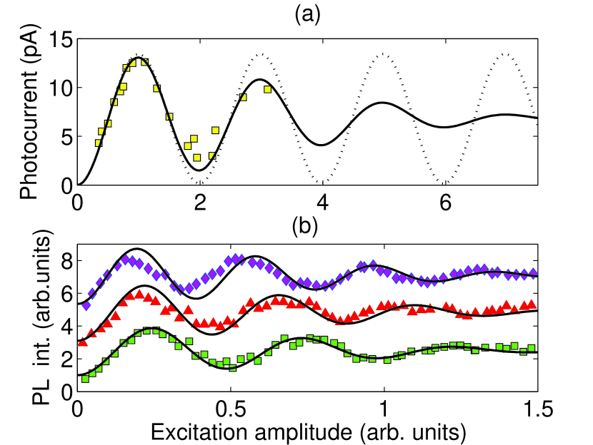
Figure 1: (a) Rabi oscillations of the photocurrent, at resonance, as a function of the excitation amplitude. The dotted line is the solution given by the Markovian Bloch equations with the dephasing rate independent of the driving field, whereas the solid line corresponds to the solution of the Bloch equations with the driving-dependent dephasing rate and generalized Rabi frequency given by Eqs. (10) and (11). Full squares represent experimental data from Zrenner et al exper , for a pulse width of about 1 ps. Here, a $\pi$-pulse corresponds to the unit of the excitation amplitude; (b) ROs in the photoluminescence (PL) intensity, at resonance, with full theoretical curves corresponding in descending order to pulse widths of 9.3 ps, 7.0 ps, and 5.4 ps, respectively. Calculations are performed with the driving-dependent dephasing rate and generalized Rabi frequency as in (a). Full symbols are the corresponding experimental data from Wang et al no-biexciton .

We now consider that the coherent driving-pulse applied to the TLS may also influence its surroundings. If the action of the driving field on the system surroundings is weak, the $K(\tau-t)$ stationary contribution to the reservoir will essentially have the same dependence on the driving-field intensity as described above. We note that the driving-pulse action on the reservoir may also give rise to non-Markovian effects stemming from the $P(\tau,t)$ non-stationary part of the reservoir’s correlation function, and that observable manifestations of these effects may be very similar to those described above. Let us illustrate it with a simple model of a bosonic reservoir driven by the same rectangular pulse that is applied on the TLS under investigation. Using the RWA, one may describe the whole ”TLS + reservoir” system with the following Hamiltonian

$$H_{1}(t) = H_{0}(t)+H_{res}(t)$$ (12)

$$+ \hbar\sigma^{+}\sigma^{-}\sum\limits_{j}[g_{j}\,b_{j}^{+}e^{i\omega_{L}(t-t_{0})}+h.c.],$$

where $H_{res}(t)$ is the reservoir Hamiltonian,

$$H_{res}(t)=\hbar\sum\limits_{j}\Delta_{j}b_{j}^{+}b_{j}+\sum\limits_{j}\Omega_{j}(t)(b_{j}^{+}+b_{j}),$$ (13)

and the $g_{j}$ are interaction constants, the $\Delta_{j}$ are detunings of the reservoir modes from the driving field, and the $\Omega_{j}$ are Rabi frequencies for every particular reservoir mode (we assume them to be constant, $\Omega_{j}(t)\equiv\Omega_{j}$, for the pulse duration). Using the interaction picture with respect to $H_{res}(t)$, one recovers from Eq. (12) the Hamiltonian of Eq. (1) with the following reservoir operator

$${\bf R}(t)=\sum\limits_{j}g_{j}\,[b_{j}+\frac{\Omega_{j}}{\Delta_{j}}]\,e^{i(\Omega_{L}+\Delta_{j})(t_{0}-t)}+h.c.\,,$$ (14)

and with the system’s detuning shifted due to the interaction with the excited reservoir, i.e., $\Delta\rightarrow\Delta-2\sum\limits_{j}g_{j}{\Omega_{j}/\Delta_{j}}$. For the reservoir initially at the vacuum state, one obtains

$$\langle{\bf R}(t)\rangle=\sum\limits_{j}g_{j}{\Omega_{j}\over\Delta_{j}}e^{i(\Omega_{L}+\Delta_{j})(t_{0}-t)}+h.c.\,,$$ (15)

and the reservoir correlation function $\langle{\bf R}(\tau){\bf R}(t)\rangle$ as the sum of a stationary part $K(\tau-t)=\sum\limits_{j}g_{j}^{2}e^{i(\Omega_{L}+\Delta_{j})(t-\tau)}$ with a non-stationary part $P(\tau,t)=\langle{\bf R}(\tau)\rangle\langle{\bf R}(t)\rangle$. The stationary part $K(\tau-t)$ produces effects already described above, and here we assume that $K(w)$ is wide and smooth enough so that the stationary dephasing rate, $\kappa_{s}$ , is independent of the intensity of the driving field. Then, from Eq. (5), one has

$$\kappa(t)=\kappa_{s}+\langle{\bf R}(t)\rangle\int\limits_{t_{0}}^{t}d\tau\langle{\bf R}(\tau)\rangle D_{++}(\tau-t).$$ (16)

Note that the non-stationary part of the dephasing rate $\kappa(t)$ decays with time [see Fig. 2(a)], since $\langle{\bf R}(t)\rangle\rightarrow 0$ for $t\rightarrow\infty$, and that the function $\langle{\bf R}(t)\rangle$ may decay slower than the stationary part, $K(t)$, of the reservoir’s correlation function as the driving field excites different modes of the reservoir in a different way, and the spectral density of the reservoir’s excitation may therefore be much narrower than $K(w)$. Moreover, in experiments on ROs in localized semiconductor systems one deals with short driving pulses, so that the non-stationary part of the dephasing rate may play a significant part in the system’s dynamics. Even if one assumes $D_{++}(t)\approx 1$ for the time-interval of interest, the non-stationary part of the dephasing rate will be dependent on the driving-field intensity. This is a purely non-Markovian dynamical effect producing an intensity-dependent damping of ROs [cf. Fig. 2(b)] quite similar to those described before.

The decrease of the dephasing rate with time may be responsible for the constant value of the dephasing rate as measured after the application of the driving pulse in the experimental measurements by Patton et al int_indep [this situation is illustrated in Fig. 2(a)]. Also, it may explain the decreased dephasing rate after the application of the pulse as in the experiment by Wang et al no-biexciton . To conclude, a driving-dependent damping of ROs due to the non-stationary contribution of the reservoir’s correlation function may take place for quite general reservoirs. Indeed, the nature of the reservoir influences only the particular form of $P(\tau,t)$ and not its general properties, which determine the effect in question.

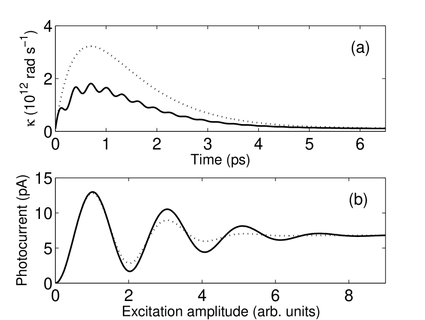
Figure 2: Examples of (a) dephasing rate $\kappa(t)$ [cf. Eq. (16)], and (b) upper-state population dynamics, for the fixed time moment corresponding to the end of the rectangular pulse, versus excitation amplitude, for a model apn-works $\langle{\bf R}(t)\rangle\sim\gamma\Omega e^{-\gamma(t-t_{0})}$, with $\gamma=2\,ps^{-1}$. Dotted lines correspond to $D_{++}(\tau-t)=1$ whereas solid lines correspond to the $D_{++}(\tau-t)$ defined in Eq. (7).

Summing up, we have demonstrated that the damping of ROs with the driving-field intensity in localized semiconductor systems (QDs, shallow donors, etc) is an effect of a very general nature, and a consequence of non-Markovian effects due to the coupling of the system to a reservoir. The exact nature of a reservoir (being an ensemble of phonons, other localized systems, traps, free carriers in a wetting layer, coupling to bi-excitons or higher decaying levels, etc, or a combination of mechanisms) is not of particular importance for the manifestation of the effect. Similar damping of ROs may occur as a consequence of different physical mechanisms. The first one stems from stationary properties of the reservoir whereas the second one is a purely non-stationary effect occurring when the driving field excites the reservoir with a decay time of the non-stationary part of the reservoir’s correlation function comparable to the driving-field pulse length.

The authors gratefully acknowledge partial financial support by EU under EQUIND project of 6FP IST-034368 and INTAS, and by Brazilian Agencies CNPq, FAPESP, Rede Nacional de Materiais Nanoestruturados/CNPq, MCT - Millenium Institute for Quantum Information, and MCT - Millenium Institute for Nanotechnology.

References

- (1) B. E. Cole, J. B. Williams, B. T. King, M .S. Sherwin, and C. R. Stanley, Nature (London) 410, 60 (2001).
- (2) A. Zrenner, E. Beham, S. Stufler, F. Findels, M. Bichler, G. Abstreiter, Nature 418, 612 (2002).
- (3) Q. Q. Wang, A. Muller, P. Bianucci, E. Rossi, Q. K. Xue, T. Takagahara, C. Piermarocchi, A. H. MacDonald, and C. K. Shih, Phys. Rev. B 72, 035306 (2005).
- (4) B. Patton, U. Woggon, and W. Langbein, Phys. Rev. Lett. 95, 266401 (2005).
- (5) A. Berthelot, I. Favero, G. Cassabois, C. Voisin, C. Delalande, Ph. Roussignol, R. Ferreira and J. M. Gerrard, Nature Physics 2, 11, 758 (2006).
- (6) S. Ya. Kilin and A. P. Nizovtsev, J. Phys. B: At. Mol. Phys. 19, 3457 (1986); P. A. Apanasevich, S. Ya. Kilin, A. P. Nizovtsev, and N. S. Onischenko, J. Opt. Soc. Am. B 3, 587 (1986); J. Appl. Spectr. 47, 1213 (1987).
- (7) For a recent review, see Y. Tanimura, J. Phys. Soc. Jap. 75, 082001 (2006).
- (8) J. Förstner, C. Weber, J. Danckwerts, and A. Knorr, Phys. Rev. Lett. 91, 127401 (2003).
- (9) A. Vasanelli, R. Ferreira, G. Bastard, Phys. Rev. Lett. 89, 216804 (2002).
- (10) L. Besombes, J. J. Baumberg, and J. Motohisa, Semicond. Sci. Technol. 19, 148 (2004); J. M. Villas-Boas, S. E. Ulloa, and A. O. Govorov, Phys. Rev. Lett. 94, 057404 (2005).
- (11) H. S. Brandi, A. Latgé, and L. E. Oliveira, Phys. Rev. B 68, 233206 (2003); H. S. Brandi, A. Latgé, Z. Barticevic, L. E. Oliveira, Solid State Commun. 135, 386 (2005).
- (12) P. Bianucci, A. Muller, and C. K. Shih, Q. Q. Wang and Q. K. Xue, C. Piermarocchi, Phys. Rev. B 69, 161303(R) (2004).
- (13) X. Li, Y. Wu, D. Steel, D. Gammon, T.H. Stievater, D.S. Katzer, D. Park, C. Piermarocchi, and L.J. Sham, Science 301, 809 (2003).
- (14) A. Royer, Phys. Rev. A 6, 1741 (1972); H.-P. Breuer, B. Kappler and F. Petruccione Phys. Rev. A 59, 1633 (1999).
- (15) R. R. Puri, Mathematical Methods of Quantum Optics, Berlin: Springer, 2001.
- (16) M. Florescu and S. John, Phys. Rev. A 69, 053810 (2004).