The VIMOS-VLT Deep Survey (VVDS)

Abstract

Aims. We present a measurement of the dependence of galaxy clustering on galaxy stellar mass at redshift $z\sim 0.9$, based on the first-epoch data from the VVDS-Deep survey.

Methods. Concentrating on the redshift interval $0.5<z<1.2$, we measure the projected correlation function, $w_{p}(r_{p})$, within mass-selected sub-samples covering the range $\sim 10^{9}$ and $\sim 10^{11}\leavevmode\nobreak\ M_{\odot}$. We explore and quantify in detail the observational selection biases due to the flux-limited nature of the survey, both from the data themselves and using a suite of realistic mock samples constructed by coupling the Millennium Simulation to semi-analytic models. We identify the range of masses within which our main conclusions are robust against these effects. Serious incompleteness in mass is present below $\log(M/M_{\odot})=9.5$, with about two thirds of the galaxies in the range $9<\log(M/M_{\odot})<9.5$ that are lost due to their low luminosity and high mass-to-light ratio. However, the sample is expected to be 100% complete in mass above $\log(M/M_{\odot})=10$.

Results. We present the first direct evidence for a dependence of clustering on the galaxy stellar mass at a redshift as high as $z\sim 0.85$. We quantify this by fitting the projected function $w_{p}(r_{p})$ with a power-law model. The clustering length increases from $r_{0}=2.76_{-0.15}^{+0.17}\leavevmode\nobreak\ h^{-1}\leavevmode\nobreak\ Mpc$ for galaxies with mass $M>10^{9}\leavevmode\nobreak\ M_{\odot}$ to $r_{0}=4.28_{-0.45}^{+0.43}\leavevmode\nobreak\ h^{-1}\leavevmode\nobreak\ Mpc$ when only the most massive ($M>10^{10.5}\leavevmode\nobreak\ M_{\odot}$) are considered. At the same time, we observe a significant increase in the slope, which over the same range of masses, changes from $\gamma=1.67_{-0.07}^{+0.08}$ to $\gamma=2.28_{-0.27}^{+0.28}$.

Comparison to the SDSS measurements at $z\sim 0.15$ shows that the evolution of $w_{p}(r_{p})$ is significant for samples of galaxies with $M<10^{10.5}\leavevmode\nobreak\ M_{\odot}$, while it is negligible for more massive objects. Considering the growth of structure, this implies that the linear bias $b_{L}$ of the most massive galaxies evolves more rapidly between these two cosmic epochs. We quantify this effect by computing the value of $b_{L}$ from the SDSS and VVDS clustering amplitudes and find that $b_{L}$ decreases from $1.5\pm 0.2$ at $z\sim 0.85$ to $1.33\pm 0.03$ at $z\sim 0.15$, for the most massive galaxies, while it remains virtually constant ($b_{L}\sim 1.3$) for the remaining population. Qualitatively, this is the kind of scenario expected for the clustering of dark-matter halos as a function of their total mass and redshift. Our result seems therefore to indicate that galaxies with the largest stellar mass today were originally central objects of the most massive dark-matter halos at earlier times, whose distribution was strongly biased with respect to the overall mass density field.

1 Introduction

In the currently accepted scenario, galaxies are thought to form within extended dark matter halos (White & Rees,, 1978), which grow through subsequent mergers in a hierarchical fashion. A major challenge in testing this general picture is to connect the observable properties of galaxies to those of the dark-matter halos in which they are embedded, as predicted, e.g., by large n-body simulations (e.g. Springel et al.,, 2006).

At the current epoch, the observed clustering of galaxies is found to depend significantly on their specific properties, such as luminosity (Hamilton,, 1988; Iovino et al.,, 1993; Maurogordato & Lachieze-Rey,, 1991; Benoist et al.,, 1996; Guzzo et al.,, 2000; Norberg et al.,, 2001, 2002; Zehavi et al.,, 2005), color or spectral type (Willmer et al.,, 1998; Norberg et al.,, 2002; Zehavi et al.,, 2002), morphology (Davis & Geller,, 1976; Giovanelli et al.,, 1986; Guzzo et al.,, 1997) and stellar mass (Li et al.,, 2006). Similar conclusions are drawn at high redshift from deep galaxy surveys (Coil et al.,, 2006; Pollo et al.,, 2006; Phleps et al.,, 2000, 2006; Meneux et al.,, 2006; Daddi et al.,, 2003).

It is somewhat natural to expect that quantities such as luminosity and, in particular, stellar mass of galaxies should in some way be related to the mass of the dark-matter halo. At the time of observation, this is strictly true only for isolated galaxies (Skibba et al.,, 2007), but moving back along the evolutionary path of the galaxy one can always find a time when this was true, before the galaxy and its halo were accreted by a larger dark-matter structure.

Recent theoretical works seem to indicate that, indeed, there exists a fairly direct relationship between global galaxy properties (e.g. their stellar or total baryonic mass, or their luminosity) and the halo mass, before it is accreted by a larger dark-matter halo ($M_{\rm infall}$, Conroy et al.,, 2006; Wang et al.,, 2006, 2007). In practice, this represents the mass of the dark matter halo of the galaxy, at a time when this was still the dominant central object of its own halo. Sensibly enough, it is $M_{\rm infall}$ which is defining the global properties of the baryonic component. This complex relation between galaxies and the (sub)halos in which they reside (Springel et al.,, 2001; Gao et al.,, 2004) offers a novel way to interpret the observed clustering properties of galaxies. Theoretically, it provides also more direct physical insight into the origin of the observed relationships, with respect to standard Halo Occupation Distribution (HOD) models (see Cooray & Sheth,, 2002).

Observationally, stellar mass has become a quantity measured with increasing accuracy, thanks to surveys with multi-wavelength photometry, extending to the near-infrared (e.g. Rettura et al.,, 2006), although some uncertainties related to the detailed modelling of stellar evolution remain (Pozzetti et al.,, 2007). This makes studies of clustering as a function of stellar mass possible for large statistical samples. Li et al., (2006) have measured the dependence of clustering on stellar mass (and other properties) in the local Universe, using a sample of $\sim 200,000$ galaxies drawn from the Sloan Digital Sky Survey (SDSS). They find, not surprisingly, that galaxies of larger mass are more clustered than low-mass ones, with the effect increasing above the characteristic knee value $M^{*}$ of the Schechter mass function. These measurements represent a high-quality reference to which high-redshift measurements can be compared to test evolution.

In studying the clustering of galaxies at different redshifts, a selection based on mass should also reduce the typical “progenitor” biases intrinsic when using flux-limited samples to study evolution of large-scale structure. Given the strong luminosity evolution between redshift zero and one, and its dependence on galaxy spectral type (Zucca et al.,, 2006), stellar mass should guarantee a more stable parameter on the basis of which comparing galaxies of possibly similar sort. If stellar mass does not evolve appreciably below $z\sim 1$ and the merger rate is also negligible in the same range (which might not be true, see Bell et al., (2006)), the growth of clustering observed for objects of fixed mass should reflect directly the evolution of the clustering of parent dark-matter halos. In fact, the stellar content of galaxies is also thought to evolve between $z=1$ and now, but this should correspond to a maximum increase in mass of a factor of 2 (Arnouts et al.,, 2007). A further complication to this idealized scenario, comes from the fact that galaxy surveys are inevitably flux-limited. Therefore, when extracting mass-selected samples, especially at high redshift, particular care has to be taken in considering selection effects that might bias the final results, essentially loosing high mass-to-light ratio galaxies at low mass (see Li et al., (2006) for discussion and correction of these effects at $z\sim 0$).

Using the VIMOS-VLT Deep Survey (VVDS), we have the possibility to investigate for the first time the evolution with redshift of the clustering in a mass-selected galaxy sample. On one side, the VVDS-Deep (see 2.1 below), gives us the opportunity to compute accurate stellar masses, by virtue of its multi-band coverage that extends to the near-infrared (see Pozzetti et al., (2007) for detailed discussion on the accuracy and intrinsic limitations of mass estimates). On the other hand, it provides us with an unprecedented area coverage for its depth ($I_{AB}\leq 24$), thus allowing the measurement of spatial statistics like the first (mean density) and second moments (two-point correlation function) of the galaxy distribution.

Closely related to this study is the work of Pollo et al., (2006), where the dependence of clustering on galaxy $B-band$ luminosity at $<z>\simeq 1$ has been measured using the VVDS. They show that at this epoch, luminous galaxies show not only a higher clustering than faint objects (similar to what is observed in the local Universe), but that their correlation function is much steeper than local counterparts. Since the $B$-band is sensitive to emission from young stars, comparison to the results presented in this paper is of interest to understand how star formation and stellar mass assembly relate to the evolution of the local environment (and vice-versa).

In the present paper, we show the first measurement of the two point correlation function as a function of stellar mass at redshift $z\sim 0.85$, for galaxies more massive than $10^{9}\leavevmode\nobreak\ M_{\odot}$. The paper is organized as follows. We introduce the data, the way stellar masses are derived and our galaxy samples in Sect. 2. We present the mock catalogues used throughout this paper in Sect. 3. The projected correlation function and its computation is introduced in Sect. 4. We discuss the stellar mass completeness of our sample and its effect on the measurement of clustering properties in Sect. 5. Results are presented in Sect. 6. Summary and conclusions are in Sect. 7.

Throughout this paper we use a Concordance Cosmology with $\Omega_{m}=0.3$ and $\Omega_{\Lambda}=0.7$. The Hubble constant is normally parametrised via $h=H_{0}/100$ to ease comparison with previous works. Stellar masses are quoted in unit of $h=1$. All correlation length values are quoted in comoving coordinates.

2 Data

2.1 The VVDS survey

The VIMOS-VLT Deep Survey (VVDS) is performed with the VIMOS multi-object spectrograph at the ESO Very Large Telescope (Le Fèvre et al.,, 2003) and complemented with multi-color BVRIJK imaging data obtained at the CFHT and NTT telescopes (McCracken et al.,, 2003; Le Fèvre et al.,, 2004; Iovino et al.,, 2005; Radovich et al.,, 2003). For this work, we use the so-called “first epoch” data, collected in the F02 “VVDS-Deep” field. This is a purely magnitude limited sample to $I_{AB}=24$, covering an area of $0.49$ square degrees with a mean sampling of $\sim 23\%$. Considering only galaxies with secure ($>80\%$ confidence) measurements, this sample includes $6530$ redshifts, with an rms accuracy (estimated from repeated observations) of 275 km s^-1. This is the same data set used in all previous clustering analyses of the VVDS. Details about observations, data reduction, redshift measurement and quality assessment can be found in Le Fèvre et al., 2005a .

2.2 Mass-limited sub-samples

Stellar masses for all galaxies in the VVDS catalogue were estimated by fitting their Spectral Energy Distribution (SED), as sampled by the VVDS multi-band photometry, with a library of stellar population models based on Bruzual & Charlot, (2003). Two different histories of star formation were used, a smooth one and a complex one with secondary bursts to derive two set of galaxy stellar mass. The initial mass function of Chabrier, (2003) was adopted in each case. The resulting typical error on stellar mass determination is $\sim$0.1 dex (depending on redshift and stellar mass). The reader is referred to Pozzetti et al., (2007) for a full description of the methodology used to derive the stellar masses and for a discussion of their robustness and intrinsic errors. In the next sections, we shall use stellar masses computed using a complex star formation history only. In practice, we found that the derived clustering properties are not sensitive to the details of the method used.

To measure the dependence of clustering on stellar mass at $z\sim 1$, similarly to Pollo et al., (2006), we have restricted the VVDS-Deep data to the redshift interval $[0.5-1.2]$. In this range, containing 4285 redshifts, we have constructed a set of mass-limited sub-samples, as defined in Tab. 1. These include four differentially binned samples, D1, D2, D3 and D4, with narrow mass ranges corresponding respectively to $\log(M/M_{\odot})$=[9.0-9.5], [9.5-10.0], [10.0-10.5], and [10.5-11.0]. We also consider four integrated samples, I1, I2, I3 and I4, including galaxies with mass larger than a given limit. While the former are useful for direct comparison to local SDSS measurements (Li et al.,, 2006), results from the integral samples are more robust, given their larger size. As we shall discuss in detail in Sect. 5, the lower-mass samples are affected, to different degrees, by incompleteness due to the primary selection in observed flux, and the scatter in the mass-luminosity relation. A large part of the following analysis will be dedicated to understanding this incompleteness and its effect on the measured clustering. These tests make extensive use of numerical simulations, described in the following section.

Table 1: Description of the 8 VVDS samples defined in the redshift range z=[0.5-1.2]

Sample	Stellar mass ($\log(M/M_{\odot})$)		Mean	Number of
	range	median	redshift	galaxies
D1	$\ \ 9.0-\ \ 9.5$	9.25	0.83	1221
D2	$\ \ 9.5-10.0$	9.71	0.83	957
D3	$10.0-10.5$	10.22	0.84	670
D4	$10.5-11.0$	10.70	0.87	329
I1	$\geq\ \ 9.0$	9.68	0.84	3218
I2	$\geq\ \ 9.5$	10.03	0.84	1997
I3	$\geq 10.0$	10.38	0.85	1040
I4	$\geq 10.5$	10.72	0.87	370

3 Simulated mock catalogues

We have built two sets of 40 mock VVDS surveys, starting from semi-analytic galaxy catalogues obtained by applying the prescriptions of De Lucia & Blaizot, (2007) to the dark-matter halo merging trees extracted from the Millennium simulation (Springel et al.,, 2005). The Millennium run contains $N=2160^{3}$ particles of mass $8.6\times 10^{8}\leavevmode\nobreak\ h^{-1}\leavevmode\nobreak\ M_{\odot}$ in a cubic box of size $500h^{-1}\leavevmode\nobreak\ Mpc$. The simulation was built with a $\Lambda$CDM cosmological model with $\Omega_{m}=0.25$, $\Omega_{\Lambda}=0.75$, $\sigma_{8}=0.9$ and $H_{0}=73km\leavevmode\nobreak\ s^{-1}\leavevmode\nobreak\ Mpc^{-1}$. For details on the semi-analytic model, we refer to De Lucia & Blaizot, (2007) and reference therein. Note that this model uses the Bruzual & Charlot, (2003) population synthesis model and a Chabrier, (2003) Initial Mass Function (IMF) to assign luminosities to model galaxies. Our mass estimates are based on the use of the same population synthesis model and IMF (Pozzetti et al.,, 2007).

The two sets of 40 $1\times 1$ deg² light cones were generated with the code MoMaF (Blaizot et al.,, 2005) for 40 independent lines of sight. The first set is complete in redshift up to $z\sim 1.7$ and contains all galaxies irrespective to their apparent magnitude or stellar mass, down to the simulation limit (that corresponds roughly to a stellar mass of $10^{8}\leavevmode\nobreak\ M_{\odot}$). We refer to these as the full mocks. They will be used to quantify the stellar mass incompleteness and its effect on clustering measurements. Nevertheless, these mocks can not be used to built observed VVDS-like mock catalogues because do not include galaxies above $z\sim 1.7$. On the other hand, the second set is complete in apparent magnitude up to $I_{AB}=24$ and was generated independently to the first one. We refer to these mock catalogues as the I24 mocks and will use them to quantify statistical errors on clustering measurement, using the full spectroscopic VVDS-02h observing strategy.

The Millennium simulation is particularly appropriate as a test-bench for the VVDS data, as it is able to reproduce a number of basic properties of the data, in particular, the number counts in various bands. Additionally, when the VVDS selection function is applied, the average redshift distribution of the mock samples is in very good agreement with the VVDS.

Most importantly for the analysis of this paper, the mass-luminosity relation of the simulated samples matches fairly well that of the data. This is shown in Fig. 1 in three redshift bins within the studied range. The general agreement between the envelopes of the observed and simulated relationships is quite encouraging, given the complexity and approximated nature of the semi-analytic models. There are clearly some differences, which will have to be taken into account when using the simulation to interpret some of the effects that are present in the data. The most evident one is an apparent excess of massive and luminous objects in the mock catalogues, in particular in the most distant redshift bin. This will not affect our conclusions when using the simulations to understand the level of incompleteness in mass due to the flux limit of the survey. This test depends on the objects with high mass-to-light ratio, near the lower luminosity limit of the data. From the three panels, we can at least say that the scatter in the relations for the data and the mocks at these luminosities is very similar. We have good reasons to hope, therefore, that the results of our tests based on the mocks will provide realistic indications on the completeness of the data. A more detailed comparison between properties of mock catalogues and VVDS data will be addressed in future papers.

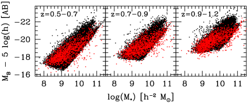
Figure 1: Comparison of the stellar mass vs. rest-frame B band relation in 3 redshift ranges between mock catalogues (black points) and VVDS data (red points).

4 Estimating the real-space correlation function

4.1 Methodology

The two-point correlation function is the simplest estimator used to quantify galaxy clustering, being related to the second moment of the galaxy distribution, i.e. its variance. In practice, it describes the excess probability to observe a pair of galaxies at given separation, with respect to that of a random distribution (Peebles,, 1980). Here we shall use the redshift-space correlation function $\xi(r_{p},\pi)$ . In this case, galaxy separations are split into the tangential and radial components, $r_{p}$ and $\pi$, as account for redshift-space distortions (Davis & Peebles,, 1983).

The real-space correlation function $\xi_{R}(r)$ can be recovered by projecting $\xi(r_{p},\pi)$along the line-of-sight, as

$$w_{p}(r_{p})\equiv 2\int_{0}^{\infty}\xi(r_{p},\pi)dy=2\int_{0}^{\infty}\xi_{R}\left[(r_{p}^{2}+y^{2})^{1/2}\right]dy$$ (1)

For a power-law correlation function, $\xi_{R}(r)=(r/r_{0})^{-\gamma}$, this integral can be solved analytically and fitted to the observed $w_{p}(r_{p})$, and find the best-fitting values of the correlation length $r_{0}$ and slope $\gamma$ (e.g. Davis & Peebles, (1983)). In computing $w_{p}(r_{p})$, the upper integration limit has, in practice, to be chosen finite, to include all the real signal without adding extra noise (which is dominant above a certain $\pi$). In our previous works, we have performed extensive experiments (Pollo et al.,, 2005), and found that, for the same data, an integration limit of $\pi_{max}=20$ h^-1Mpc provides the best compromise in terms of noise and systematic bias of the result. Using 30 or 40 h^-1Mpc does not change the recovered $w_{p}(r_{p})$ appreciably, while increasing the scatter. Finally, fitting $w_{p}(r_{p})$ for separations $<10$ $h^{-1}$ Mpc using the procedure described in detail in Pollo et al., (2005), that takes into account the covariance matrix of the data and in particular the fact that the bins are not fully independent, provides a best-fitting value of $r_{0}$ and $\gamma$ for each mass-selected sub-sample.

To measure in practice $\xi(r_{p},\pi)$ from each data sample, we use the standard estimator of Landy & Szalay, (1993):

$$\xi(r_{p},\pi)=\frac{N_{R}(N_{R}-1)}{N_{G}(N_{G}-1)}\frac{GG(r_{p},\pi)}{RR(r_{p},\pi)}-\frac{N_{R}-1}{N_{G}}\frac{GR(r_{p},\pi)}{RR(r_{p},\pi)}+1$$ (2)

where $N_{G}$ is the mean galaxy density (or, equivalently, the total number of objects) in the survey; $N_{R}$ is the mean density of a catalogue of random points distributed within the same survey volume and with the same selection function as the data; $GG(r_{p},\pi)$ is the number of independent galaxy-galaxy pairs with separation between $r_{p}$ and $r_{p}+dr_{p}$ perpendicular to the line-of-sight and between $\pi$ and $\pi+d\pi$ along the line of sight; $RR(r_{p},\pi)$ is the number of independent random-random pairs within the same interval of separations and $GR(r_{p},\pi)$ represents the number of galaxy-random cross pairs.

4.2 Correction of observational biases

To properly estimate the correlation function from the VVDS data, we need to correct for the different sampling rate, which on average is 22.8% but varies with the position on the sky due to the VIMOS foot-print and the superposition of multiple passes (Le Fèvre et al., 2005a, ). To this end, in Pollo et al., (2005) we developed and tested a correction scheme based on computing a specific local weight around each galaxy with measured redshift. The weight is computed utilizing the angular information of the “missed” galaxies contained in the survey parent photometric catalogue, which should have the same redshift distribution as the spectroscopic sample. In our specific case, in which we are considering the clustering of galaxies within a given mass range, the parent photometric catalogue should contain only galaxies in the same range. This information is a priori not available, as to compute it one needs to know galaxy distances. As a remedy to this, we used the photometric redshifts that have been measured to very good accuracy ($\sigma_{\Delta z/(1+z)}=0.029$ for our redshift range), over the whole VVDS-02h Deep field (Ilbert et al.,, 2006), thanks to the combination of CFHT-LS and VVDS photometry. This uncertainty on the galaxy distance corresponds to an error on the computed stellar mass of $\sim$0.16dex (Pozzetti et al.,, 2007). The chosen redshift range is large enough to assume that edge effects due to photometric redshift errors are marginal. We stress that here we are not using the photometric redshifts directly into the correlation estimate, but only in the correction weight, to assign the galaxy to the appropriate (broad) redshift slice and mass interval. We used this information to build, for each mass-selected spectroscopic data set, a corresponding mass-selected parent photometric catalogue containing galaxies in the range $0.5\leq zphot\leq 1.2$. This method allowed us to simplify the weight expression originally used for the overall flux-limited sample (equation 12, Pollo et al.,, 2005), such that the the $i$-th galaxy will have a weight

$$w_{i}=\sqrt{\frac{n_{p}(i)(n_{p}(i)-1)}{n_{s}(i)(n_{s}(i)-1)}}\,\,\,\,.$$ (3)

In this expression, $n_{p}$ is the total number of galaxies in the parent catalogue inside a circle of fixed radius [chosen to be 40^′′ on the basis of mock experiments (Pollo et al.,, 2005)], centred on the $i$-th galaxy, while $n_{s}$ is the number of spectroscopically-observed galaxies inside the same area. The idea behind this weighting scheme is that a pair of galaxies will contribute to the correlation function with a total weight $w_{i}w_{j}$, proportional to the ratio of the expected-to-measured numbers of pairs within the chosen radius.

Since the sub-samples analyzed in this work are essentially volume-limited (above the mass completeness limit discussed in the next section), we do not need to apply any other weighting scheme as usually done for purely flux-limited surveys [as e.g. in Li et al., (2006)].

4.3 Systematic and statistical errors on correlation estimates

To test for biases in our correction scheme and to quantify statistical errors on the estimates of $w_{p}(r_{p})$, we used the 40 I24 mocks catalogues described in Sect. 3. From the full $1\times 1\leavevmode\nobreak\ deg^{2}$ light-cones, we created 40 fully realistic VVDS-02h surveys, by applying the entire selection function and observing strategy of the real data as described in Pollo et al., (2005). For each of the 40 cones, therefore, we had the possibility to measure both the “true $I_{AB}\leq 24$” and “observed” values of $w_{p}(r_{p})$ and the corresponding power-law-fit parameters to the spatial correlation function. Comparing the mean and rms of the difference in the measured parameters, we find that (on the average, over the four mass ranges), the recovered value of $r_{0}$ is 5% accurate (the maximum systematic effect found in the case of the I1-like set of mocks, is 10%); similarly, the slope $\gamma$ is consistent with no systematic bias, and a scatter of 4%. These conclusions are similar to those in Pollo et al., (2005). Finally, the root-mean-square variation of $w_{p}(r_{p})$ among the 40 “observed” mocks provides us with an estimate of the error bars on our measurements of $w_{p}(r_{p})$, $r_{0}$ and $\gamma$. Assuming the simulations are a realistic representation of reality, these error bars also include cosmic variance from fluctuations on scales larger than the sample size.

5 Effects of mass incompleteness

The VVDS flux limit in the $I$ band translates at different redshifts into different lower luminosity limits. This, in turn, translates into a broad mass selection cut at each redshift, reflecting the scatter in the Mass-Luminosity relation. If not treated appropriately, this introduces a bias against high mass-to-light (ML) ratio galaxies, i.e. objects that would enter the sample if this were purely mass selected, but that are excluded simply because they are too faint to fulfill the apparent magnitude limit. Furthermore, at a fixed luminosity in the observed band, it will be the redder objects (typically more clustered), dominated by low-luminosity stars, to have the highest ML ratios and thus to be preferentially excluded (see Fig. 4). If this is not accounted for in some way, it will inevitably affect the estimated clustering properties, with respect to a truly complete, mass-selected sample. It is therefore necessary to understand in detail the effective completeness level in stellar mass of the samples that we have defined for our analysis. We have explored this issue using two complementary and independent approaches based respectively on the data themselves and on the mock samples. The latter will also allow us to test directly the effects of the incompleteness on the measured clustering; the results of this test will be presented in Sect. 5.3.

5.1 Observed scatter in the mass-luminosity relation

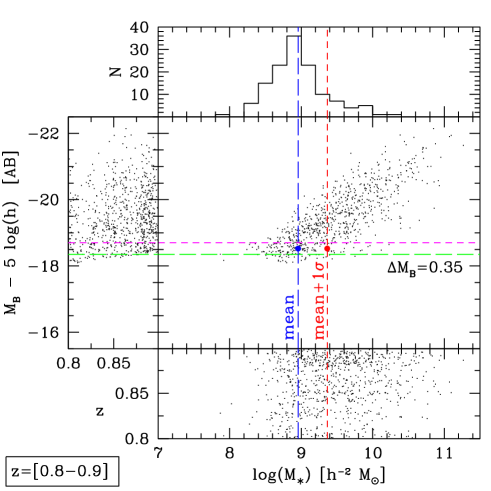
Figure 2: Construction of the completeness limit from VVDS data in the narrow redshift range z=[0.8-0.9]. The central panel shows the value of B-band luminosity vs. the computed stellar mass for all galaxies in that redshift range. The long-dashed horizontal line defines the minimum galaxy luminosity above which stand 95% of the galaxies. The top horizontal dashed line defines the upper limit in which we compute the mean and standard deviation of the stellar mass distribution of galaxies (top panel) standing in a luminosity interval of $\Delta M_{B}=0.35$. The right-hand dashed vertical line defines the 84% completeness limit in stellar mass.

A first way to understand the incompleteness in mass of our samples is to measure directly the scatter in the mass-luminosity relation near the flux limit of the survey and from this estimate the fraction of missing objects, at the given mass limit. Since the flux limit of the survey translates into a different luminosity limit at different redshifts, we need to do this in narrow redshift ranges as to track the change of the incompleteness within the broad redshift range of the sample (and also take into account any potential evolution in the Mass-Luminosity relation). The method is illustrated by Fig. 2 where we plot the value of B-band luminosity vs. the computed stellar mass for all galaxies in the redshift range z=[0.8-0.9]. The “completeness” limit, defined as the value of stellar mass above which virtually all masses, given the observed distribution, are included in the sample is estimated as follows: 1) given a redshift bin ($\Delta z=0.1$), we compute the minimum galaxy luminosity detected at that distance, defined as the value of absolute magnitude above which we have 95% of the galaxies, $M_{min}$; this is given by the long-dashed horizontal line of Fig. 2. 2) We then consider a luminosity interval $[M_{min};M_{min}-0.35]$, chosen as the minimum thickness to provide us with statistics sufficient to define the properties – mean and scatter – of the (logarithmic) mass distribution, as indicated by the short-dashed horizontal line in the same figure. We shall define for a specific redshift the completeness limit to be:

$$Y_{c}(z)=\left<Y(z)\right>+\sigma_{Y}(z)\,\,\,,$$ (4)

where $Y(z)=\log M(z)$. Note that the completeness limit defines, as a function of $z$, the value of mass above which, given the selection properties of the survey, a sample will be better than 84% complete in mass (corresponding to one-sided $1\sigma$ limit). Note that here we do not have enough data to perform a refined Gaussian reconstruction as done by Li et al., (2006) for the SDSS. The completeness locus as a function of redshift is plotted as the bold (red) solid line in Fig. 3 in the plane redshift-mass. Figure 3 indicates that any sample limited to masses larger than $10^{9.5}M_{\odot}$ will be fairly complete in stellar mass over the whole redshift range we plan to explore. This completeness limit is consistent with the one derived by Pozzetti et al., (2007) in the redshift range [0.9-1.2] in the determination of the galaxy stellar mass function from the VVDS data (see their Fig. 9).

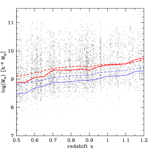
Figure 3: Distribution of stellar masses as a function of redshift, in the range [0.5-1.2]. The top (bold) solid line, computed from the observed scatter in the luminosity-mass relation, defines the limit above which samples are better than 84% complete. The bottom line defines the 50% completeness limit. The two dashed lines represent the same limits but derived from the Millennium simulation.

5.2 Mass incompleteness from the mock catalogues

Encouraged by the realistic appearance of the Mass-Luminosity relation for our mock samples (Fig. 1), we can try and use them to independently test the consistency of the incompleteness level estimated in the previous section.

As a first test, we can apply to the mock samples the direct technique used on the data in the previous section. The results of this, averaged over the 40 mock samples, are shown in terms of a completeness curve in the plane $z-M$ in Fig. 3 (dashed lines). Interestingly, we see that the 84% completeness level obtained from the simulations is very close to that from the data (upper curve), although the mean values of the two mass-luminosity relationships are slightly different.

Then, let us exploit the full mock catalogues defined in Sect. 3, which are deeper than the magnitude limit of the VVDS and include galaxies with stellar mass down to $10^{9}\leavevmode\nobreak\ M_{\odot}$. It is therefore possible to quantify independently the fraction of galaxies we miss when applying the VVDS selection function, provided that the Mass-Luminosity relation and its scatter are comparable in the data and in the simulations. We have seen from Sect. 3 that this is quite a reasonable assumption.

We define, for a given mass selection, the completeness $C$ as the fraction of objects recovered when the apparent magnitude selection $17.5\leq I_{AB}\leq 24$ is applied, with respect to the pure mass-selected sample. The average values of $C$ among the 40 full mocks catalogues are reported in Tab. 2 for z=[0.5-1.2].

Table 2: Mean fraction of galaxies in the redshift range z=[0.5-1.2] for which $17.5\leq I_{AB}\leq 24$ among 40 mocks catalogues (serie S1) which are complete in stellar mass down to $10^{9}\leavevmode\nobreak\ M_{\odot}$, built from the Millennium simulation with semi-analytical model of De Lucia & Blaizot, (2007)

$\log(M/M_{\odot})$	C
$\ \ 9.0-\ \ 9.5$	0.37
$\ \ 9.5-10.0$	0.70
$10.0-10.5$	0.93
$10.5-11.0$	0.99
$\geq\ \ 9.0$	0.56
$\geq\ \ 9.5$	0.79
$\geq 10.0$	0.94
$\geq 10.5$	1.00

These values indicate that for $9<\log(M/M_{\odot})<9.5$, our sample is strongly incomplete, with an expected value of lost galaxies larger than 60%. This represents an average value over the z=[0.5-1.2] redshift range (while we have seen from the previous analysis that the incompleteness is actually a function of redshift). More encouragingly, the tests also show that an integral sample with $\log(M/M_{\odot})>9.5$ is already $\sim 80\%$ complete and that samples above $\log(M/M_{\odot})=10$ are better than 93% complete both in the differential and integral cases. It is interesting to use the simulated sample to explore which are the properties of the “missed” galaxies. Figure 4 shows the luminosity and rest-frame (B-I) color distributions of galaxies fainter than $I_{AB}=24$ but with masses in the range $\log(M/M_{\odot})=[9.0-9.5]$, compared to those brighter than this limit (and thus retained within the sample). Interestingly, the population missed by the VVDS selection function – at least for the mock samples – is fairly red galaxies, as one would expect for higher-than-average mass-luminosity ratio objects dominated by old stars.

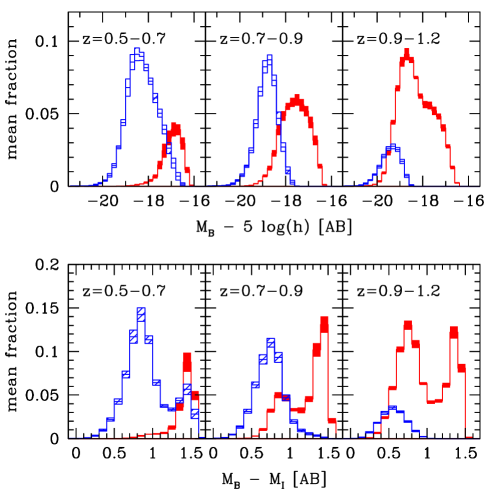
Figure 4: Mean luminosity and color distributions, with their $1\sigma$ variance, for galaxies with stellar masses in the range $\log(M/M_{\odot})=[9-9.5]$ in the full millennium mock catalogues, for 3 consecutive redshift ranges between $z=0.5$ and $z=1.2$. Solid red distributions correspond to galaxies fainter than $I_{AB}=24$, while hatched blue distributions correspond to galaxies brighter than this threshold. The distribution have been normalized to the total number of galaxies in each redshift range. The galaxies missed due to the $I_{AB}=24$ flux limit function are clearly intrinsically fainter and relatively redder.

Finally, considering the differential 84% completeness limit in Fig. 3, we note that – once averaged over the redshift range – it roughly corresponds to a mass limit $\log(M/M_{\odot})>[9.5-10]$. This is consistent with the integral completeness fraction $C$ derived in this section using the simulations, for the same range of masses (Table 2).

5.3 Effects on the measured clustering

We can use the 40 full mock catalogues to go one step further and directly quantify the effects of the mass incompleteness on the clustering measurements, when compared to purely mass-selected samples.

Figure 5 shows the average and scatter over the 40 mocks of the ratio of the projected functions measured respectively with and without the VVDS flux limit, within the usual mass ranges.

Figure 5: Effect of mass incompleteness on the projected correlation function $w_{p}(r_{p})$ estimated using the Millennium mock catalogues for the 8 mass ranges . The points give at each scale $r_{p}$ the mean ratio of the correlation functions $w_{p}(r_{p})$ measured for a sample complete in stellar mass and its corresponding sub-sample selected in apparent magnitude $17.5\leq I_{AB}\leq 24$. Error bars correspond to the rms scatter among the mocks.

As expected, the values of $w_{p}(r_{p})$ are significantly affected by the mass incompleteness, in particular at very small separations. For samples containing masses below $\log(M/M_{\odot})\sim 10$, not only the amplitude is underestimated by 15% or worse, but also the shape of $w_{p}(r_{p})$ is affected, with the average ratio becoming smaller and smaller below $1\leavevmode\nobreak\ h^{-1}\leavevmode\nobreak\ Mpc$. This can be translated in terms of a systematic bias in the measurements of $r_{0}$ and $\gamma$. The results of averaging the relative difference $\delta x/x=(x_{true}-x_{obs})/x$ over the 40 mocks, are reported in Tab. 3 in terms of a relative bias $\epsilon(x)=<\delta x/x>_{40}$ on each parameter. In all cases the mass incompleteness produces a systematic underestimate of both the amplitude and slope of $\xi(r)$.

In particular, we have a systematic $\sim 25\%$ underestimate of the correlation length $r_{0}$ in the lowest-mass sample ($\log(M/M_{\odot})=[9.0-9.5]$). The slope $\gamma$ is less affected (7%); this is related to the fact that the fit is performed out to $r_{p}=10$ h^-1 Mpc, and thus is not so sensitive to the small-scale flattening that is evident in Fig. 5. We also see that the systematic effect is significantly less severe for the integral samples (e.g. only 6% on $r_{0}$ and 3% on $\gamma$ for $\log(M/M_{\odot})\geq 9.5$).

On the basis of these extensive tests, we shall consider as reliable in the analysis of the VVDS data only results for samples with a minimum mass limit of $\log(M/M_{\odot})=9.5$, with some caution also in interpreting the results from the sample D2 ($9.5<\log(M/M_{\odot})<10$), which is still affected by some residual incompleteness.

In the next section, we shall present the measured values in general uncorrected for these effects, but will discuss and show how they would change assuming a correction for the incompleteness as derived in Tab. 3. All plotted error bars on the measured points will correspond to the statistical uncertainty only, as estimated from the variance in the 40 I24 mock catalogues.

Table 3: Average systematic underestimate of the clustering length $r_{0}$ and the slope $\gamma$ of the correlation function introduced by the mass incompleteness. The values are computed for each parameter as $\epsilon(x)\leavevmode\nobreak\ =\leavevmode\nobreak\ <\delta x\leavevmode\nobreak\ /\leavevmode\nobreak\ x>_{40}$, where $\delta(x)\leavevmode\nobreak\ =\leavevmode\nobreak\ x_{true}-x_{observed}$ and the average is performed over 40 mock samples.

$\log(M/M_{\odot})$	average underestimate
	$\epsilon(r_{0})$	$\epsilon(\gamma)$
$\ \ 9.0-\ \ 9.5$	25%	7%
$\ \ 9.5-10.0$	11%	3%
$10.0-10.5$	3%	1%
$10.5-11.0$	0%	0%
$\geq\ \ 9.0$	13%	5%
$\geq\ \ 9.5$	6%	3%
$\geq 10.0$	2%	1%
$\geq 10.5$	0%	0%

6 Results

6.1 $w_{p}(r_{p})$ as a function of mass at $z\sim 0.85$

Figure 6 shows the projected correlation function $w_{p}(r_{p})$ computed for the four samples I1 to I4 (left panel) and its best fit parameters together with their $1-$, $2-$ and $3\sigma$ error contours derived from the 40 I24 observed mock catalogues (right panel). The measured values of $r_{0}$ and $\gamma$ for each sample are reported for convenience also in Tab. 4, including those for the sample D1 for which we know that the incompleteness is severe. No correction for incompleteness is applied to the plotted values

Even accounting for the effect of incompleteness and the size of the error contours, we observe a clear increase of the amplitude and the slope of the correlation function for increasing median stellar mass, even if error contours are quite large in the highest mass range where the statistics is poor (Tab. 1). This trend is also quite clear in Fig. 7 where instead we have used the simulation results to correct (open symbols) the observed values (filled symbols), dividing them by $(1-\epsilon(x))$ (Tab. 3). Note how especially for the integral samples (right panels), the trend with increasing mass is quite robust and significant. We thus conclude that already at $z\sim 0.9$ higher mass galaxies are significantly more clustered than lower mass objects, with a systematic trend both in the amplitude and slope of the spatial correlation function. This dependence on stellar mass is coherent in general terms with the trend found as a function of luminosity (Pollo et al.,, 2006).

Table 4: Clustering length and slope of the correlation function $w_{p}(r_{p})$ for the different samples in the redshift range z=[0.5-1.2]. Values are derived for $0.2\leq r_{p}\leq 21\leavevmode\nobreak\ h^{-1}.Mpc$. Associated errors have been extrapolated from the variance measured among 40 mocks catalogues for each stellar mass range. Values have not been corrected by underestimate due to stellar mass incompleteness.

Sample	$\log(M/M_{\odot})$	$r_{0}$ ($h^{-1}.Mpc$)	$\gamma$
D1	$\ \ 9.0-\ \ 9.5$	$2.55_{-0.25}^{+0.25}$	$1.65_{-0.12}^{+0.13}$
D2	$\ \ 9.5-10.0$	$3.45_{-0.31}^{+0.32}$	$1.79_{-0.14}^{+0.14}$
D3	$10.0-10.5$	$3.54_{-0.34}^{+0.33}$	$1.88_{-0.15}^{+0.16}$
D4	$10.5-11.0$	$4.35_{-0.47}^{+0.46}$	$1.96_{-0.24}^{+0.27}$
I1	$\geq\leavevmode\nobreak\ \leavevmode\nobreak\ 9.0$	$2.76_{-0.15}^{+0.17}$	$1.67_{-0.07}^{+0.08}$
I2	$\geq\leavevmode\nobreak\ \leavevmode\nobreak\ 9.5$	$3.24_{-0.20}^{+0.21}$	$1.77_{-0.08}^{+0.09}$
I3	$\geq 10.0$	$3.72_{-0.27}^{+0.29}$	$1.88_{-0.12}^{+0.12}$
I4	$\geq 10.5$	$4.28_{-0.45}^{+0.43}$	$2.28_{-0.27}^{+0.28}$

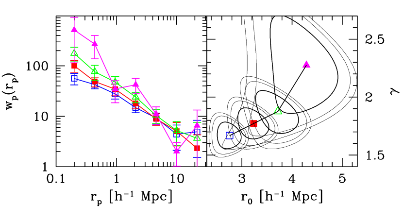
Figure 6: (Left) Measurements of the projected correlation function $w_{p}(r_{p})$ of galaxies with different stellar masses: $\log(M/M_{\odot})\geq 9.0$ (open blue squares), $\geq 9.5$ (filled red squares), $\geq 10.0$ (open green triangles) and $\geq 10.5$ (filled magenta triangles) from VVDS data in the redshift range [0.5-1.2]. (Right) The best-fit parameters ($r_{0}$ and $\gamma$) with their associated $1-$, $2-$ and $3\sigma$ error contours, derived from the variance among 40 mock catalogues. In this plot, no correction for the effect of incompleteness in mass is applied (see text). Note however that the correction would affect both $r_{0}$ and $\gamma$ and, for example, move the open square (the most affected one) in the right panel without modifying the observed trend.

Figure 7: Correlation length and slope measured from VVDS data at $z\sim 0.85$ as a function of the median stellar mass of each samples. Left and right panels refer respectively to the differential and integrated samples. Filed symbols indicate measurement non-corrected by stellar mass incompleteness, while open symbols are.

6.2 Comparison to SDSS

This segregation in term of stellar mass at redshift $z\sim 0.85$ is also observed at low redshift in the SDSS data (Li et al.,, 2006). These authors present their result directly in terms of the measured amplitude of $w_{p}(r_{p})$ on different physical scales because of the departure of the correlation function from a pure power law observed by numerous authors (e.g.  Guzzo et al.,, 1991; Zehavi et al.,, 2004). In Fig. 8 we plot our measurements of $w_{p}(r_{p})$ at $z\sim 0.85$ together with those by Li et al., (2006) at $z\sim 0.15$ within the three mass ranges in which we have established that the incompleteness does not strongly affect the measurements. A reference power-law $w_{p}(r_{p})$, corresponding to $r_{0}=5$ h^-1 Mpc and $\gamma=1.8$ is over-plotted for reference. Blue open circles correspond to correcting the observed values of $w_{p}(r_{p})$ according to the results of Fig. 5.

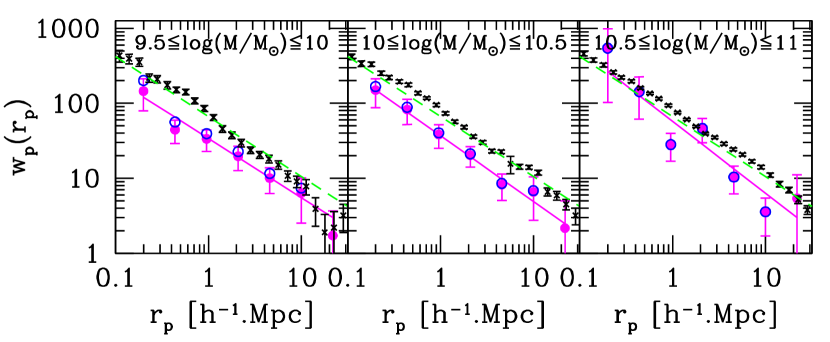
Figure 8: Comparison of the projected correlation function $w_{p}(r_{p})$ from SDSS data at z$\sim$0.15 (black cross; Li et al.,, 2006) to VVDS measurement at z$\sim$0.85 (magenta filled dots and solid lines) in 3 differential ranges of stellar masses. The green dashed line is a power-law reference line drawn with $r_{0}=5$ h^-1.Mpc and $\gamma=1.8$. Error bars on VVDS measurement have been estimated from the variance among 40 mock catalogues. Blue open circles indicate VVDS measurements corrected for stellar mass incompleteness.

Figure 8 not only shows the dependence of galaxy clustering on stellar mass at a given redshift but also, at the same time, the evolution of the amplitude and shape of the correlation function $w_{p}(r_{p})$ with redshift for a given stellar mass range. The observed evolution is apparently faster for low-mass objects than for massive ones: the amplitude of $w_{p}(r_{p})$ increases by a factor $\sim$2-3. Conversely, in the high-mass range, $\log(M/M_{\odot})=[10.5-11.0]$, the amplitudes at $z\sim 0.85$ and $z\sim 0.15$ are very similar, within the error bars. These results hold even when considering corrections to the projected function accounting for the stellar mass incompleteness (blue empty circles, Fig. 8).

6.3 Comparison to model predictions

So far, we have used the mock VVDS surveys built from the Millennium Simulation to assess where our results are reliable against the survey selection effects and established the range of stellar masses where this is plausibly the case. In this section we would like to exploit more fully their intrinsic scientific content. As discussed previously, these mock samples were constructed by populating dark matter halos from the Millennium Run (Springel et al.,, 2005), using the latest version of the Munich semi-analytic model (De Lucia & Blaizot,, 2007). We have shown this model is in quite agreement with a number of observational results. As we already discussed, the “ideal” light cones were “observed” to produce realistic replicas of the VVDS-Deep survey, with the same sampling, field pattern and incompleteness. They are therefore ideal for providing a direct comparison, under the same conditions, to the $w_{p}(r_{p})$measured from the VVDS data. This is shown in Fig. 9, where the data points are compared to the average of the measurements from the 40 observed mock samples (solid line), including a $\pm 1\sigma$ error corridor. The agreement of the data and the model predictions for the redshift range considered, $0.5<z<1.2$, is rather good for all three mass ranges explored. The VVDS points are consistent with the predictions of the semi-analytic model within $1\sigma$ or better. A more comprehensive comparison of these models with the clustering of VVDS galaxies as a function of different properties (luminosity, color, spectral type), will be presented in a separate paper.

Finally, we also note that a similar dependence on stellar mass is also predicted in the hydrodynamical simulations of Weinberg et al., (2004), in which the steepening of the correlation function is particularly marked on scales below $0.5h^{-1}Mpc$.

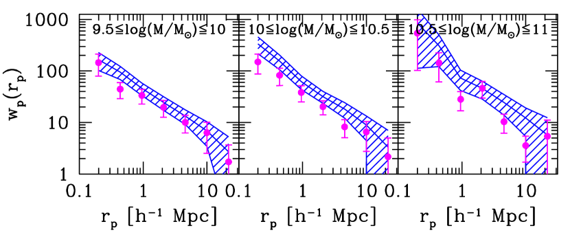
Figure 9: Comparison of the VVDS measurements of the projected correlation function $w_{p}(r_{p})$ as a function of stellar mass (filled circles), with that obtained from 40 mock VVDS surveys constructed from the Millennium Simulation. The dashed area describes the rms among the 40 simulated catalogues.

6.4 Evolution on galaxy bias

Our results suggest that the apparent evolution of clustering from $z\sim 1$ to the current epoch has been stronger for the less massive galaxies than for the most massive ones. In other words, the relative bias of massive to less-massive galaxies was larger at $z\sim 1$ than it is today. This behavior is also fairly well reproduced by the Millennium mocks.

In the currently standard scenario of galaxy formation, galaxies form and evolve inside dark matter haloes (White & Rees,, 1978), with the first objects appearing inside the most massive of these. These are expected to correspond to the highest, more rare fluctuations of the overall matter density field. On simple statistical grounds, it can be shown that these peaks will be more clustered than the general dark matter distribution, i.e. they will be biased (Kaiser,, 1984). Thus, from very simple considerations, if a larger stellar mass corresponds to a larger hosting dark matter halo mass, then the most massive galaxies at high redshift will correspond to the highest peaks and will be highly biased. Strong clustering and high bias are observed both for massive spheroidals at redshifts in the range $z\sim 1.5-2.5$, selected on the basis of their red optical-infrared colors (e.g. Daddi et al.,, 2003), and for strongly star-forming galaxies at $z\sim 3$ selected from their strong UV Lyman break (e.g. Steidel et al.,, 2004).

Another important piece of information is that, when selected on the basis of a fixed rest-frame luminosity, galaxies show an increase of their average bias as a function of redshift. Using the VVDS data, we have in particular shown that the bias of galaxies with $M_{b}\leq-20+5\log{\rm h}$ increases by a factor $\sim 1.5$ between $z=0$ and $z\sim 1.5$ (Marinoni et al.,, 2005). However, we also know that the typical luminosity of the general population of galaxies increases by more than a magnitude over the same redshift range, which implies that at a fixed absolute luminosity we are in fact looking at different populations of objects at different redshifts. Given that there is clear evidence for at most a factor of 2 increase in the stellar mass between $z=0$ and $z=1$ (Arnouts et al.,, 2007), the analysis presented here has the virtue of addressing the dependence of clustering with respect to a more physical and stable property of the galaxy population. Even by allowing for a factor of 2 increase in the mass (i.e. assuming that the progenitors of objects with mass $\bar{M}$ at $z\sim 0$ are galaxies with mass $\bar{M}/2$, at $z\sim 1$), our results would not change significantly.

It is therefore of interest to interpret in a more quantitative way our findings, by estimating the evolution of the linear bias for galaxies with similar mass at different redshifts. In Marinoni et al., (2005) we showed that the bias is in fact non-linear, at about the 10% level. This has very little effect on the present discussion, and we can safely assume here a linear bias model for $b_{L}$, where the galaxy rms fluctuations $\sigma_{R,g}$ on a given scale $R$ can be expressed as

$$\sigma_{R,g}=b_{L}\sigma_{R,m}\,\,\,\,.$$ (5)

with $\sigma_{R,m}$ the mass rms fluctuations on the same scale. We also make the further assumption that the bias $b_{L}$ is independent of scale, which is very reasonable on sufficiently large scales. It is customary to express the rms fluctuation of galaxies and mass in spheres of radius $R=8$ h^-1Mpc, with the value of $\sigma_{8,m}$ adopted as standard expression for the normalization of the mass power spectrum at the present epoch. Here we adopt the value $\sigma_{8,m}=0.76$ (Spergel et al.,, 2007). This value at $z=0$ can be scaled to the epochs of interest here by considering the growth of fluctuations in our assumed model, $\sigma_{8,m}(z)=\sigma_{8,m}(z=0)D(z)$, where $D(z)$ is the linear growth factor of density fluctuations, $D(z)=g(z)/[g(0)(1+z)]$, and the normalized growth factor $g(z)$ can be approximated as (Carroll et al.,, 1992; Mo & White,, 2002)

$$g(z)\approx{5\over 2}\Omega_{\rm m}\left[\Omega_{\rm m}^{4/7}-\Omega_{\Lambda}+(1+\Omega_{\rm m}/2)(1+\Omega_{\Lambda}/70)\right]^{-1}\,\,\,\,,$$ (6)

with $\Omega_{\rm m}$ and $\Omega_{\Lambda}$ the density parameters in non relativistic matter and cosmological constant. Note that in this expression,

$$\Omega_{\rm m}(z)={\Omega_{\rm m,0}(1+z)^{3}\over E^{2}(z)}\,,\leavevmode\nobreak\ \leavevmode\nobreak\ \leavevmode\nobreak\ \leavevmode\nobreak\ \leavevmode\nobreak\ \Omega_{\Lambda}\equiv\Omega_{\Lambda}(z)={\Omega_{\rm\Lambda,0}\over E^{2}(z)}\,.$$ (7)

with $\Omega_{\rm m,0}$ and $\Omega_{\rm\Lambda,0}$ their present-day values and

$$E^{2}(z)=\left[\Omega_{\rm\Lambda,0}+(1-\Omega_{0})(1+z)^{2}+\Omega_{\rm m,0}(1+z)^{3}\right]\,\,\,\,,$$ (8)

the normalized expansion factor.

The corresponding value of the rms galaxy fluctuations on the same scale can be estimated from the parameters of the correlation function under the assumption of a power-law form, $\xi(r)=(r_{0}/r)^{\gamma}$ (Peebles,, 1980), as

$$\sigma_{8,g}=\sqrt{C_{\gamma}\left(\frac{r_{0}}{8Mpc/h}\right)}\,\,\,\,,$$ (9)

where

$$C_{\gamma}=\frac{72}{(3-\gamma)(4-\gamma)(6-\gamma)2^{\gamma}}\,\,\,\,.$$ (10)

To be consistent with our work at $z=0.85$, we estimated the parameters $r_{0}$ and $\gamma$ for the SDSS at $z\sim 0.15$ from the published measurements of $w_{p}(r_{p})$ by Li et al., (2006), fitting over the same range used for the VVDS ($0.18\leq r_{p}\leq 17.9h^{-1}Mpc$). The resulting values of $b_{L}$ (with $\Omega_{\rm m,0}=0.3$ and $\Omega_{\rm\Lambda,0}=0.7$) over the three mass ranges and at the two redshifts considered are plotted in Fig. 10. The values are also reported for reference in Tab. 5.

Figure 10: The redshift evolution of the linear bias for galaxies of different stellar mass, obtained from the SDSS ($z\sim 0.15$, open squares, (Li et al.,, 2006)), and the VVDS ($z\sim 0.85$, filled squares, this work).

Table 5: Measured values of the linear bias for the VVDS and SDSS samples, within 3 stellar mass ranges (see text).

Sample	$\log(M/M_{\odot})$	b(z)
		SDSS ($z\sim 0.15$)	VVDS ($z\sim 0.85$)
D2	$\ \ 9.5-10.0$	$1.26\pm 0.03$	$1.29\pm 0.10$
D3	$10.0-10.5$	$1.37\pm 0.03$	$1.32\pm 0.12$
D4	$10.5-11.0$	$1.40\pm 0.03$	$1.62\pm 0.18$

Figure 10 shows that for galaxies in the highest-mass range considered here ($10.5\leq\log(M/M_{\odot})\leq 11$), the evolution of the linear bias between redshift 0.15 and 0.85 seems stronger than for the lower mass ranges, where it is substantially constant over the same redshift range. For the high mass range, the increase in the bias going back in time corresponds to a factor $\sim 1.2$ (from $b=1.40\pm 0.03$ to $b=1.62\pm 0.18$)

This kind of behavior is generally expected for the clustering evolution of dark-matter halos of different mass. (Mo & White,, 1996; Sheth et al.,, 2001; Mo & White,, 2002). More massive halos form near the peaks of the density field, whose distribution is strongly biased with respect to the overall mass distribution and displays a higher clustering amplitude (Kaiser,, 1984). Our result therefore suggests a direct relationship (as one would naively expect), between the total mass in stars accumulated today (or at $z\sim 1$) and that of the dark-matter halo within which the bulk of the baryonic material was originally assembled. Clearly, to be still observed at these redshifts, this proportionality needs to have been preserved also through the merging events experienced by the galaxy. These produce a merging of the dark-matter halo and a parallel full coalescence of the baryonic components, with the new baryonic remnant still sitting in the center of its new, more massive halo. This is not the case when the galaxy is accreted by a much larger halo (e.g. a cluster), becoming a satellite whose own halo will be significantly disturbed and modified in mass by dynamical friction. This scenario fits well with the results of recent simulations (Conroy et al.,, 2006; Wang et al.,, 2006), that are able to reproduce the observed clustering properties of galaxies as a function of luminosity at very different redshifts (up to $z\sim 3$) by simply assuming that each dark-matter sub-halo would generate a galaxy characterized by a B-band luminosity proportional to its original “infall” mass (i.e. mass before being last accreted into a larger halo).

7 Summary and conclusions

We have used the VVDS-Deep data (Le Fèvre et al., 2005a, ) to perform a first exploration of the dependence of galaxy clustering on stellar mass at a redshift approaching unity. This has only now become possible at these epochs, thanks to the large number of redshifts and extended wavelength coverage available from VVDS-Deep that allow us to compute reliable stellar masses. We started with a sample of 3218 galaxies with $M>10^{9}\leavevmode\nobreak\ M_{\odot}$ in the redshift range $z=[0.5-1.2]$. We thoroughly investigated the completeness limit in mass of the redshift catalogue, using mock samples built from the Millennium simulation coupled to semi-analytical recipes. We have found that there is a significant mass incompleteness induced by the flux-limit of the survey below $M=10^{10}\leavevmode\nobreak\ M_{\odot}$, whose effects on the measured clustering become particularly severe below $M=10^{9.5}\leavevmode\nobreak\ M_{\odot}$. We used the mock surveys to quantify this systematic effect and to estimate realistic statistical error bars that possibly include “cosmic” variance from fluctuations on scales larger than the explored volume. With these limitations in mind, we have obtained a series of results, that can be summarized as follows:

• We have measured for the first time a clear stellar mass-dependent clustering of galaxies with respect to their stellar mass at a redshift as high as $z\sim 0.85$, with the more massive objects being more clustered than less massive ones. In particular, the most massive objects show an increase in both amplitude and slope of the spatial correlation function.

• These clustering properties are very well reproduced (within 1-$\sigma$) in the same redshift and mass ranges, by the mock samples built from the Millennium run. Together with their realistic redshift distribution, this represents a remarkable achievement of the models.

• Comparison of our measurements to the similar ones obtained (with much better statistics) from the SDSS data at $z\sim 0.15$ (Li et al.,, 2006) show evidence for a more significant change in the apparent clustering amplitude for low-mass galaxies ($\log(M/M_{\odot})\leq 10$) than in the case of the most massive objects ($\log(M/M_{\odot})\sim 11$). The correlation function of the latter, in fact, remains roughly constant with time.

• Assuming a standard cosmology, we computed the expected evolution of the root-mean-squared fluctuation in the mass, $\sigma_{8}$, between the two epochs sampled by VVDS and SDSS. Using this value, we translated the observed evolution of $w_{p}(r_{p})$ into the corresponding linear bias, showing that the most massive galaxies display an evolution of the bias factor, from $b=1.40\pm 0.03$ at $z\sim 0.15$ to $b=1.62\pm 0.18$ at $z\sim 0.85$. This finding is not unexpected in a hierarchical scenario in which the most massive peaks of the mass density field collapse earlier and evolve faster (Mo & White,, 1996). This interpretation supports a scenario in which the stellar mass of a galaxy is essentially proportional to the mass of the dark-matter halo in which it was last the central object, consistent with recent simulations (Conroy et al.,, 2006; Wang et al.,, 2006).

The combination of these measurements of clustering as a function of stellar mass and as a function of luminosity at the same redshift (Pollo et al.,, 2006), together with the analogous SDSS results at $z\sim 0.15$, can provide very important complementary constraints to models describing how galaxies are distributed within dark matter halos (Zheng et al.,, 2007). This can help us to understand the evolution of galaxies of different mass below $z\sim 1$ and in particular on the role of mergers within this redshift range.