ASTE Submillimeter Observations of a Young Stellar Object Condensation in Cederblad 110

Abstract

We present results of submillimeter observations of a low-mass young stellar objects (YSOs) condensation in the Cederblad 110 region of the Chamaeleon I dark cloud with Atacama Submillimeter Telescope Experiment. Our HCO⁺($J$=4-3) map reveals a dense molecular gas with an extent of $\sim$ 0.1 pc, which is a complex of two envelopes associated with class I sources Ced110 IRS4 and IRS11 and a very young object Cha-MMS1. The other two class I sources in this region, IRS6 and NIR89, are located outside the clump and have no extended HCO⁺ emission. HCO⁺ abundance is calculated to be $2.6\times 10^{-10}$ for MMS1 and $3.4\times 10^{-9}$ for IRS4, which are comparable to the reported value for other young sources. Bipolar outflows from IRS4 and IRS6 are detected in our ¹²CO($J$=3-2) map. The outflow from IRS4 seems to collide with Cha-MMS1. The outflow has enough momentum to affect gas motion in MMS1, although no sign has been detected to indicate that a triggered star formation has occurred.

1 INTRODUCTION

1.1 Single Star Formation and Cluster Formation

A number of past observations and theoretical researches have revealed a rough scenario for the formation of isolated, single low-mass stars. That is, a gravitational collapse of a molecular cloud core is the starting point of star formation, then a protostar with a thick envelope and bipolar outflows (Bachiller, 1996) is born. The outflows blow off the protostellar envelope, which could have an impact on the mass assembling process of the star (e.g. Arce & Goodman, 2002), affect the motion of the cloud around the protostar (e.g. Takakuwa et al., 2003), and cause outflow-triggered star formation (Yokogawa et al., 2003), as well as generates turbulence and limit the efficiency of star formation (Nakano et al., 1995; Matzner & McKee, 2000).

It is still veiled how to form stars in a group or a cluster (Lada & Lada, 2003), although most stars are known to be born that way. If stars are forming in a group or cluster, impacts of outflows on the environment may be greater than in the formation of isolated stars. Therefore, it is important to study interactions between outflows and dense gas in cluster-forming regions for comprehensive understandings of star formation processes.

1.2 Cederblad 110 Region

The Cederblad (Ced) 110 region (Cederblad, 1946) is located in the center of the Chamaeleon (Cha) I dark cloud, one of the low-mass star formation regions in the solar vicinity ($D$=160pc; Whittet et al., 1997). Haikala et al. (2005) identified a C¹⁸O clump in the Ced 110 region, whose radius is 0.19 pc and mass is 11.7 $M_{\sun}$. This is the most massive clump in their samples. Infrared and millimeter continuum observations (Prusti et al., 1991; Reipurth et al., 1996; Zinnecker et al., 1999; Lehtinen et al., 2001; Persi et al., 2001) have revealed that seven YSOs at different evolutionary stages and one very young source are clustered within $\sim$0.2 pc. In Table ASTE Submillimeter Observations of a Young Stellar Object Condensation in Cederblad 110 we list the objects with their position, IR class, $T_{\rm bol}$ (Myers & Ladd, 1993), and $L_{\rm bol}$.

The youngest object in this region, Cha-MMS1, was detected by 1.3 mm continuum observations by Reipurth et al. (1996). At this position, Lehtinen et al. (2001) identified the far-IR object Ced 110 IRS10 by observations with the Infrared Space Observatory (ISO), while no corresponding source has been detected with near-IR observations. Thus, MMS1 is considered to be a ”real protostar” (Lehtinen et al., 2001). However, Lehtinen et al. (2003) could not detect 3 or 6 cm radio continuum emission. This result indicates MMS1 does not have any jets or outflows. They noted that MMS1 is still at a prestellar stage.

Ced110 IRS4, a class I object, is associated with a reflection nebula that is extended in a north-south direction and is divided by a thick edge-on dust disk (Zinnecker et al., 1999; Persi et al., 2001). Henning et al. (1993) detected 1.3 mm radio continuum emission from this object, while extended emission was not detected (Reipurth et al., 1996).

Molecular outflow was detected in this region by ¹²CO($J$=1-0) observations with the Swedish-ESO Submillimeter Telescope (SEST; Mattila et al., 1989; Prusti et al., 1991), but the identification of its driving source has been controversial. Originally, IRS4 was thought to be driving this outflow. However, Reipurth et al. (1996) detected MMS1 and suggested that MMS1 is the driving source of the outflow as well as the nearby Herbig-Haro (HH) objects HH49/50 (see also Kontinen et al., 2000). While Lehtinen et al. (2003) revealed that MMS1 is associated with no jets, Bally et al. (2006) suggested that a parsec-scale outflow is ejected from MMS1 based on the positional relationship among the HH objects and the YSOs in their large area shock survey. Lack of high-resolution mapping observations of the outflow (e.g. the mapping grid was 1$\arcmin$ in Mattila et al. 1989) have made it difficult to resolve this issue.

Ced110 IRS11 was first detected by Zinnecker et al. (1999) as IRS 4E in their near-IR image. Lehtinen et al. (2001) tentatively detected a far-IR source from ISO data, and identified IRS11 as ISO-ChaI 86 (Persi et al., 2000). The coordinates for IRS11 in Table ASTE Submillimeter Observations of a Young Stellar Object Condensation in Cederblad 110 are based on the position for ChaI 86 in Persi et al. (2001).

In this paper we focus on the following three points; (1) the distribution of dense gas in the YSO clustering region, (2) the influence of outflows from older protostars on newer ones and the surrounding gas, and (3) the ”blue asymmetry” line profile toward YSOs which indicates the existence of infalling gas (Leung & Brown, 1977; Zhou, 1992). To investigate them we observed CO($J$=3-2) and HCO⁺($J$=4-3) lines. The observations of the CO line can reveal the distribution of molecular outflows with high spatial resolution and enable us to distinguish the driving source of outflows. The HCO⁺ line has a high critical density of $9.7\times$10⁶ cm^-3 at the $J$=4-3 transition (Evans, 1999), and its observations can probe dense gas and also can detect gas infall in protostellar systems through detection of the blue asymmetry in line profiles. We also made observations of the optically thin H¹³CO⁺ line toward Ced110 IRS4 and Cha-MMS1 to obtain precise physical parameters. In addition, we observed CH₃OH($J$=$7_{K}$-$6_{K}$), SiO($J$=8-7), and SO ($J$=$8_{9}$-$7_{8}$) lines, whose upper energy levels are 70.5, 75.0, and 87.5 K, respectively. These high energy levels made these lines useful diagnostic tools of shocked regions.

We introduce the detail of our observations in §2, and the results of the observations are described in §3. In §4 we discuss molecular abundance, gas infall toward protostars, kinematics of outflows, and the interaction between MMS1 and the outflow from IRS4. Our conclusions are summarized in §5.

2 OBSERVATIONS

The CO($J$=3-2) and HCO⁺($J$=4-3) observations were performed in 2004 November with the 10 m Atacama Submillimeter Telescope Experiment (ASTE, Ezawa et al., 2004). Observations were remotely made from the ASTE operation rooms at San Pedro de Atacama, Chile and National Astronomical Observatory of Japan (NAOJ) Mitaka campus, Japan, using the network observation system N-COSMOS3 developed by NAOJ (Kamazaki et al., 2005). We used a 345 GHz (0.8 mm) band double side band (DSB) superconductor-insulator-superconductor mixer receiver using position switching. Taking advantage of the DSB observation, we simultaneously received ¹²CO($J$=3-2; 345.796 GHz) in the lower side band (LSB) and HCO⁺($J$=4-3; 356.734 GHz) in the upper side band (USB). With the same system, we observed H¹³CO⁺($J$=4-3; 346.999 GHz) line in 2005 June and the CH₃OH($J$=$7_{K}$-$6_{K}$; 338.344 GHz), SO ($J$=$8_{9}$-$7_{8}$; 346.529 GHz), and SiO($J$=8-7; 347.331 GHz) lines in 2006 December.

We used the XF digital spectrometer with a bandwidth and spectral resolution set to 128 MHz and 125 kHz, respectively, except for CH₃OH line observations made at 512 MHz bandwidth and 500 kHz resolution. The velocity resolution is 0.11 km s^-1 and 0.43 km s^-1 in 345 GHz. The half-power beamwidth (HPBW) was 22$\arcsec$ at 345 GHz.

In CO and HCO⁺ observations, the mapping grid spacing was 20$\arcsec$ (0.016 pc at the distance of Cha I). According to Mizuno et al. (1994), the typical size of a star-forming core is about 0.03 pc, thus the angular resolution of our observations is high enough to resolve this size of a core. With this grid spacing, we obtained spectra toward 136 points which resulted in 4$\arcmin\times 3\arcmin$ maps centered at IRS4. The observations were made by position switching every 20 or 30 s between the source and off positions. The off positions were ($\alpha,\delta$)(J2000) = (11${}^{\rm h}24^{\rm m}21\fs 2$, $-76\arcdeg 57\arcmin 39\farcs 1$) and ($11^{\rm h}42^{\rm m}9\fs 7$, $-78\arcdeg 03\arcmin 44\farcs 4$). These positions were checked to be free of emission.

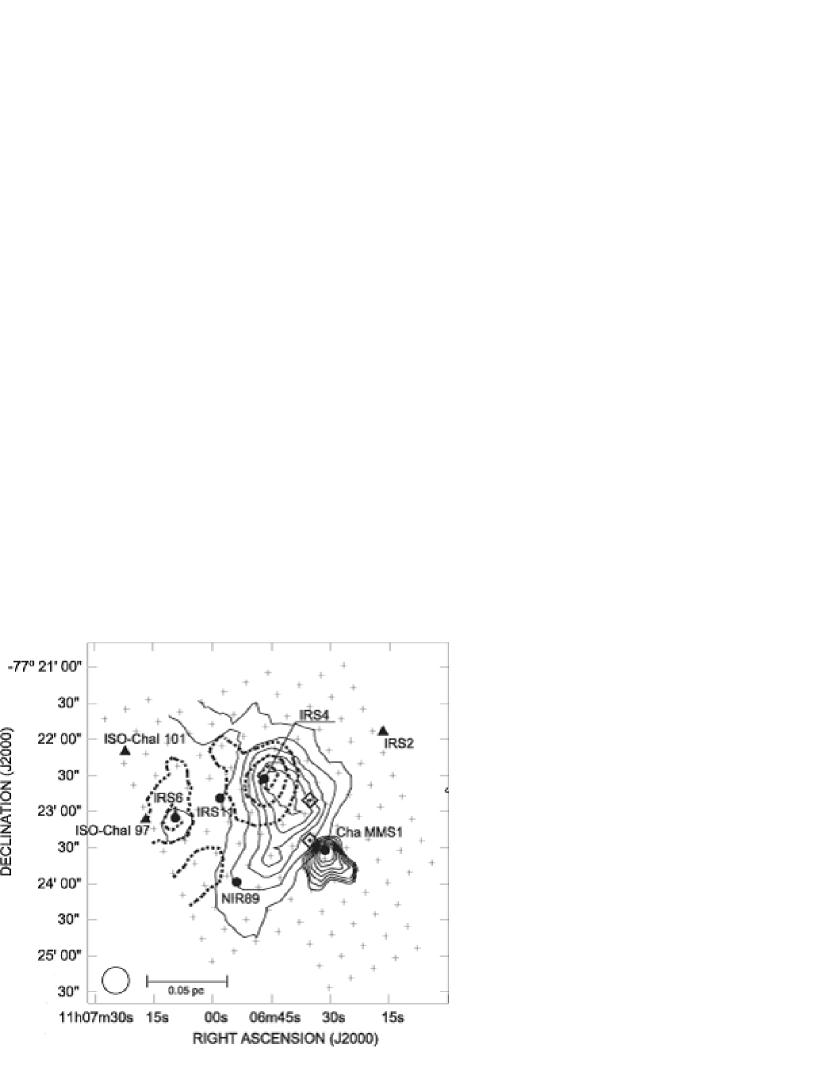
Figure 1: Distribution of high velocity component of CO($J$=3-2) line. The blueshifted (-4.0 km s^-1 $\leq V_{\rm LSR}\leq 3.0$ km s^-1) and the redshifted (6.3 km s^-1 $\leq V_{\rm LSR}\leq$ 10.3 km s^-1) components are drawn with solid and dotted lines, respectively. The first contour level and contour interval are 1.53 K km s^-1 for the blueshifted components and 1.1 K km s^-1 for redshifted components. Cha-MMS1 observed with a 1.3 mm continuum (Reipurth et al., 1996) is also shown with thick lines. The first contour level is 200 mJy, and the interval is 25 mJy. Small crosses indicate observed points. Each YSO is shown by filled circles (pre-stellar core and class I) or triangles (class II or III). The diamonds with the central dot denote the observed points of SO and SiO lines. The HPBW is indicated with an open circle.

We observed H¹³CO⁺ lines toward Ced110 IRS4 and Cha-MMS1. The CH₃OH line was observed along the line from IRS4 to MMS1 with $20\arcsec$ grid spacing. SO and SiO lines were observed simultaneously in opposite sidebands toward the Kontinen et al. (2000) SO northern peak, ($\alpha,\delta$)(J2000) = ($11^{\rm h}06^{\rm m}34\fs 7,-77\arcdeg 22\arcmin 50\farcs 7$), and the boundary point between IRS4 outflow and MMS1, ($\alpha,\delta$) (J2000) = ($11^{\rm h}06^{\rm m}34\fs 7,-77\arcdeg 23\arcmin 24\farcs 8$). The observed point for the shock-tracer molecules are indicated on Fig.1.

DSB system noise temperature at an elevation of 35$\arcdeg$ varied from $T_{\rm sys}=$ 300 to 600 K. For CO and HCO⁺ lines, on-source integration time for each point ranged from 1 to 5 minutes, and the typical rms noise was 0.3 and 0.15 K, respectively. We made additional integration toward the YSOs for improving signal-to-noise ratio in the HCO⁺ line, reaching a rms noise of 0.1 K. For other lines, we made the rms noise level go down to 0.05 K for H¹³CO⁺, 0.1 K for CH₃OH, 0.15 K for SiO, and 0.2 K for SO. Despite a careful inspection, no emissions from shock-tracing molecules such as CH₃OH, SiO, and SO were detected in our observations. All temperatures are reported in terms of the $T_{\rm MB}$ scale. The main beam efficiency was $\eta_{\rm MB}\sim 0.6$.

The telescope pointing was regularly checked by observing Jupiter, Saturn, or IRC+10216 every 1 or 2 hr during observations, and the error was estimated to be about 5$\arcsec$ peak to peak. Intensity calibration was carried out by the chopper-wheel method (Kutner & Ulich, 1981). The absolute intensity is calibrated by assuming that $T_{\rm MB}$ of IRC+10216 for CO ($J$=3-2) is 32.5 K (Wang et al., 1994). The daily variability was checked by observing L1551 IRS5 for HCO⁺ and by observing Ori KL for H¹³CO⁺, CH₃OH, SO, and SiO. The sideband ratio was assumed to be unity. The zenith 220 GHz opacity varied from $\tau\sim 0.05$ to $\sim 0.1$. Matsuo et al. (1998) reported the atmospheric transmission is 0.86 and 0.83 in 345 and 356 GHz, respectively, when the zenith 220 GHz opacity was 0.04. In this paper, we assume the atmospheric transmissions in the two side-bands are identical.

We reduced the data using the NEWSTAR software developed in the Nobeyama Radio Observatory. The baseline subtraction was done by a straight line in most cases.

3 RESULTS

3.1 Overview

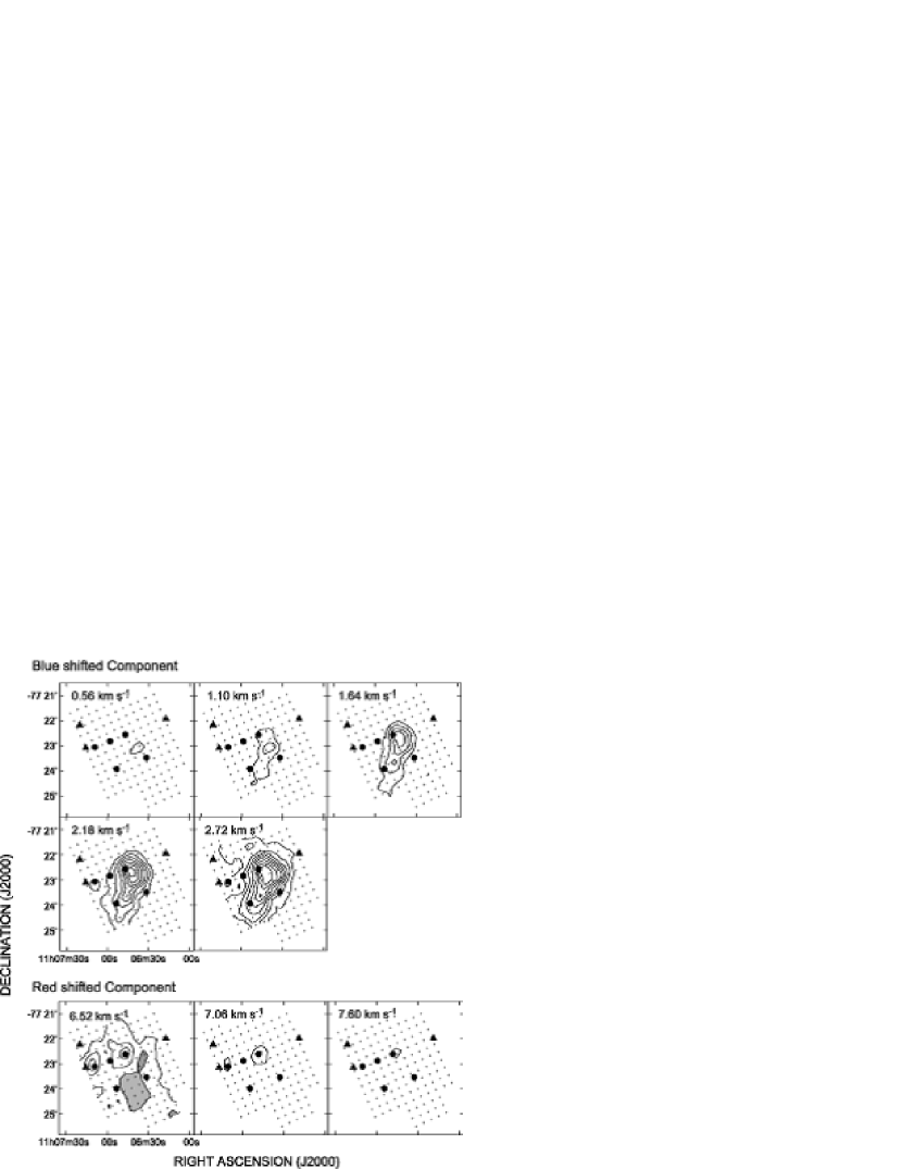
Figure 2: Velocity channel maps of CO($J$=3-2) in the outflow range. The central LSR velocity for each integral in units of km s^-1 is shown at the top left corner of each panel. The first contour level and contour interval are 0.8 K. The markers are the same as in Fig.1. The gray region represents local minimum.

Figures 1 and 2 show the observed maps of the CO($J$=3-2) emission. The CO($J$=3-2) emission was detected at all points within the 4$\arcmin\times 3\arcmin$ map with a varying degree of intensity. Around IRS4 and IRS6, we detected CO high-velocity components most probably caused by outflows. The details of the outflows are described in §3.3 and §4.3.

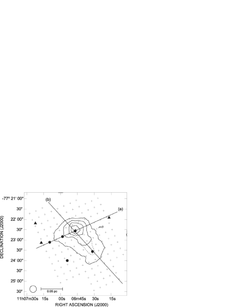
Figure 3: Integrated intensity map of Ced110 in HCO⁺($J$=4-3) and the distribution of YSOs. The integrated velocity range is 2.0 km s^-1 $\leq V_{\rm LSR}\leq$ 7.0 km s^-1. The first contour level and contour interval are 0.8 K km s^-1. Dashed line shows the ”absorption-free” integrated intensity contour (See §3.3.2). The open circle shows the HPBW. Filled circles and triangles indicate the positions of YSOs as in Fig.1. The straight lines are also shown along which the position-velocity diagrams in Fig.5 and 6 are taken.

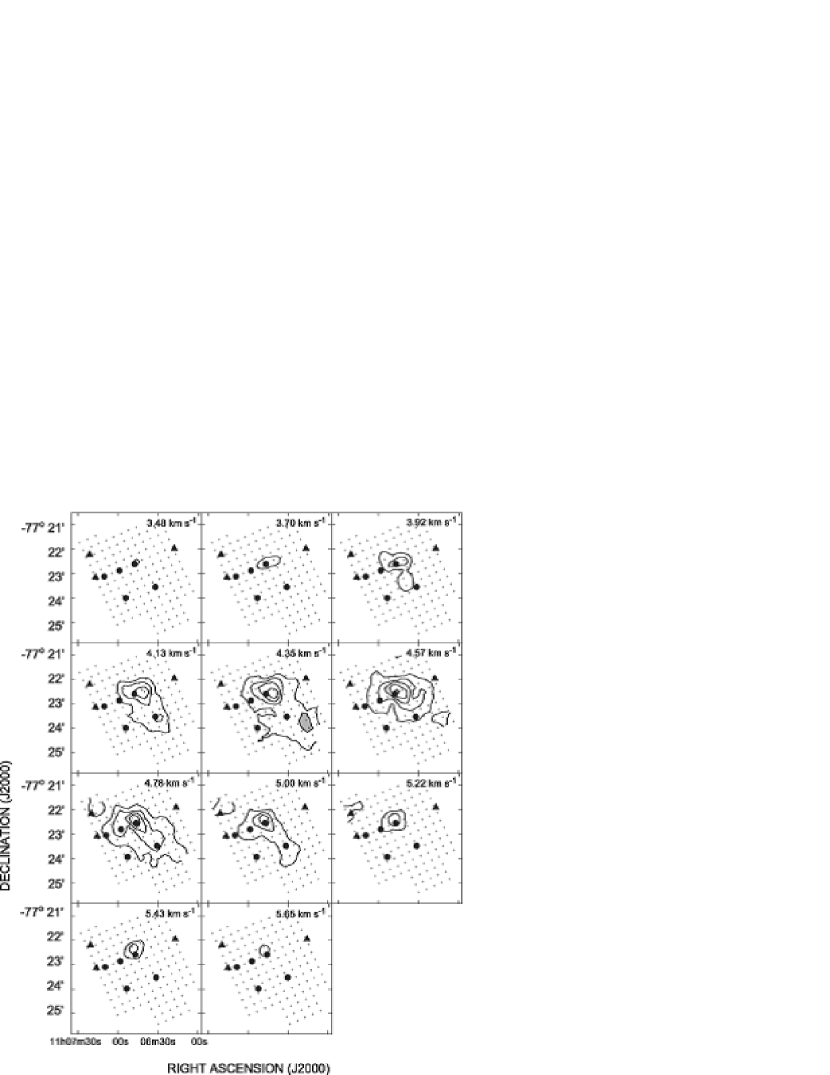
Figure 4: Velocity channel maps of HCO⁺($J$=4-3) transition. The central LSR velocity for each integral in units of km s^-1 is shown at the top right corner of each panel. The first contour level and contour interval are 0.5 K. The positions of YSOs are indicated with the same symbols as in Fig.1. The gray region represents local minimum.

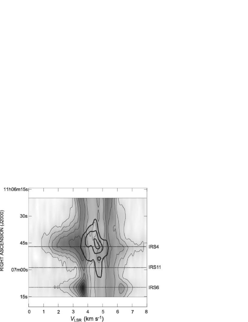
Figure 5: Position velocity diagram along the line (a) in Fig. 3. CO($J$=3-2) and HCO⁺($J$=4-3) are shown with thin and thick line, respectively. The first contour level and contour interval are 1.5 K for CO and 0.9 K for HCO⁺. The positions of IRS4, IRS6, and IRS11 are indicated with dashed lines.

Figure 3 shows the integrated intensity map of the HCO⁺($J$=4-3) line in the velocity range of 2.0 km s^-1 $\leq V_{\rm LSR}\leq$ 7.0 km s^-1. A HCO⁺ clump of dense gas is seen in Fig.3. This clump is an aggregate of three independent envelopes associated with Ced110 IRS4, IRS11, and Cha-MMS1. The envelope associated with IRS11 seems to be apart from the component associated with IRS4 in the $V_{\rm LSR}=$ 4.78 and 5.00 km s^-1 panels of Fig.4. MMS1 is also distinguishable in the $V_{\rm LSR}=$ 3.92 and 4.13 km s^-1 panels. Figure 5 and 6 are the position-velocity diagrams of CO and HCO⁺ lines along line A and B in Fig.3, respectively. In Fig.5 the components associated with IRS4 and IRS11 are marginally resolved with the viewpoint of line width, that is, the emission associated with IRS4 exhibits a distinctly larger linewidth than that for IRS11. The HCO⁺ clump covers $140\arcsec\times 110\arcsec$ (0.11 pc $\times$ 0.085 pc) above the 3 $\sigma$ noise level. The extension of the clump with a position angle $\sim 45$ deg corresponds well to the 200 $\mu$m ridge emission observed with ISO (Lehtinen et al., 2001).

3.2 CO and HCO⁺ Line Profiles

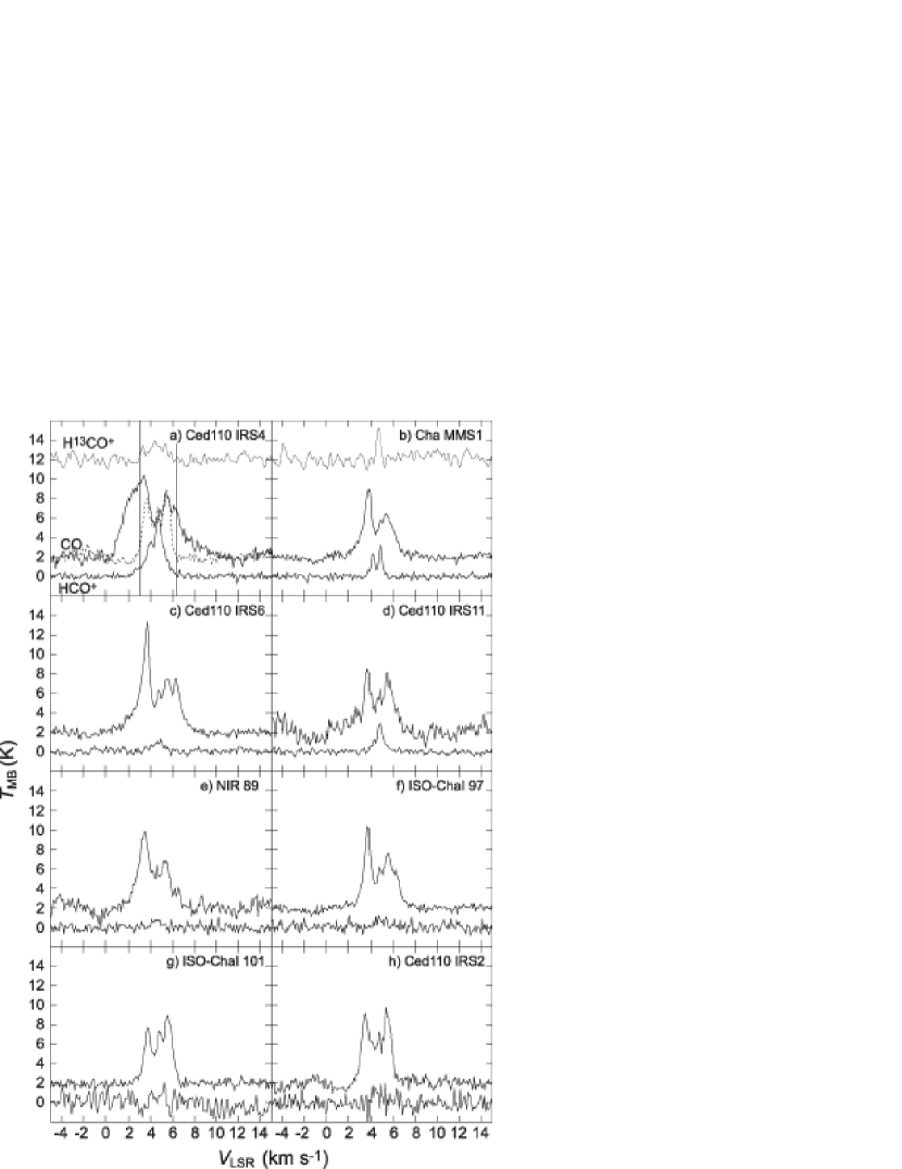
Figure 7: HCO⁺($J$=4-3) (multiplied by a factor of 2), CO($J$=3-2) (with 2 K offset), and H¹³CO⁺($J$=4-3) (only in IRS4 and MMS1 panels with 12 K offset and multiplied by a factor of 15) line profiles toward Cha-MMS1 and YSOs in Ced110 region. In panel a, the spectrum toward the edge of the map is indicated with a dotted line, and the borders between outflow and line core are shown with two vertical lines. We identified $V_{\rm LSR}\leq$ 3.0 km s^-1 and $V_{\rm LSR}\geq$ 6.3 km s^-1 as outflow.

The CO($J$=3-2), HCO⁺($J$=4-3), and H¹³CO⁺($J$=4-3) line profiles obtained at YSO positions are shown in Fig.7. The CO line profile from ambient gas is sampled at the boundary of the map and shown in Fig.7a by a dotted line.

Almost all CO line profiles have a dip at $V_{\rm LSR}\sim 4.3$ km s^-1. The dip also appears in some HCO⁺ line profiles at the same velocity. The velocity of the dip is identical to that of C¹⁸O clump number 3 identified in the Ced110 region by Haikala et al. (2005), and also gives close agreement with the velocities of optically thin lines observed by Kontinen et al. (2000). These correspondences mean that this dip is caused by self-absorption by less excited gas, not the result of two emission components with different velocities along the same line of sight. Since the observed region corresponds to one C¹⁸O clump, the outer gas of the clump in the lower excitation level would make the CO absorption. The dip in the HCO⁺($J$=4-3) line indicates a significant population of the $J=3$ level that requires a moderately high density, but with a lower $J$=4-3 excitation temperature than in the center of the clump. This is a reflection of the density gradient in the clump. We can find these dips in Fig. 5 and 6. This dip prevents the channel map (Fig.4) from representing the actual distribution of interstellar matter in the dip velocity. The indentations of contours located at the south of IRS4 and a lack of a peak around MMS1 in the panels of $V_{\rm LSR}=4.35$ and 4.57 km s^-1 of Fig.4 may be due to the self-absorption. It is conceivable that other reasons such as depletion and chemistry in the dense gas cause this lack of a peak. The issue of molecular depletion is discussed in §4.1.

The parameters of the lines detected at YSO positions are summarized in Tables 2, 3 and 4. We fitted the spectral data of HCO⁺ and H¹³CO⁺ with a Gaussian profile. The error estimates of the values in the tables come from the fit. In deriving the line parameters, the velocity ranges of outflows and self-absorption features in the lines are eliminated in the fitting processes. Although this may have some defectiveness, this is the optimal handling of our data.

3.3 Individual Sources

3.3.1 Ced110 IRS4 and the Outflow

Bipolar outflow from IRS4 is detected in our CO($J$=3-2) observations. This outflow had been also detected by Mattila et al. (1989) and Prusti et al. (1991) with their CO($J$=1-0) observations. We compared the line profiles toward IRS4 with that of the ambient gas obtained at the edge of the map in ($\alpha,\delta$)(J2000) = ($11^{\rm h}06^{\rm m}24\fs 3$, $-77\arcdeg 21\arcmin 16\farcs 7$). Judging from this comparison shown in Fig.7a, the line profile in the velocity ranges of $V_{\rm LSR}\leq 3.0$ km s^-1 and $V_{\rm LSR}\geq$6.3 km s^-1 are not affected by the ambient gas, and thus we identified these ranges as outflow components.

The distribution of the outflow components from IRS4 are shown in Fig.1 (integrated intensity map) and Fig.2 (channel map). The blueshifted and redshifted outflows show a different aspect. The spatial extent of the blueshifted outflow is considerably larger than that of the redshifted outflow. Furthermore, the highest velocity component of the blueshifted outflow lies midway between IRS4 and MMS1, while the velocity reaches its peak around IRS4 in the redshifted flow. The near-IR images (Zinnecker et al., 1999; Persi et al., 2001) indicate that IRS4 is seen nearly edge-on. The observed distribution of the blueshifted component of the outflow extending to the south suggests that the outflow axis slightly inclines with the southern side closer than the northern side. This configuration is in agreement with the previous remarks on the inclination of IRS4 based on the color gradient of the nebulae (Zinnecker et al., 1999). They found that the northern part of the reflection nebula is redder than the southern part, which suggests that the northern part is tilted away from us. Our integrated intensity map (Fig.1) does not show the redshifted component in the south of MMS1 reported in the literature (Mattila et al., 1989; Prusti et al., 1991). In the channel map (Fig.2), however, one can see the extended redshifted emission at $V_{\rm LSR}=6.52$ km s^-1, and this could be its counterpart.

Observations of the H¹³CO⁺($J$=4-3) line were also performed toward IRS4 (Fig.7a) with a 43 mK noise level. The FWHM of this line, $\Delta V=1.72\pm 0.29$ km s^-1, corresponds to that of the HCO⁺ line within the margin of error. This supports the detection of the line. With this result, we discuss molecular abundance in §4.1.

3.3.2 Cha-MMS1

In Fig.7b we show the CO, HCO⁺, and H¹³CO⁺ line profiles toward Cha-MMS1. The dip in the HCO⁺ line is deeper than that of IRS4. This deeper dip shows that MMS1 is deeply embedded in the densest part of C¹⁸O clump number 3 (Haikala et al., 2005), because MMS1 lies nearer to the position of the peak intensity of C¹⁸O than IRS4.

We calculated the HCO⁺ ”original” integrated intensity with a Gaussian fit using the line profiles in the velocity ranges which are free from self-absorption. These reconstructed ”absorption-free” contours are shown with dashed linea in Fig.3. The summit ridge of the contours extends south and reaches the position of MMS1. This result again supports the idea that MMS1 is deeply embedded and its outer envelope makes this absorption feature.

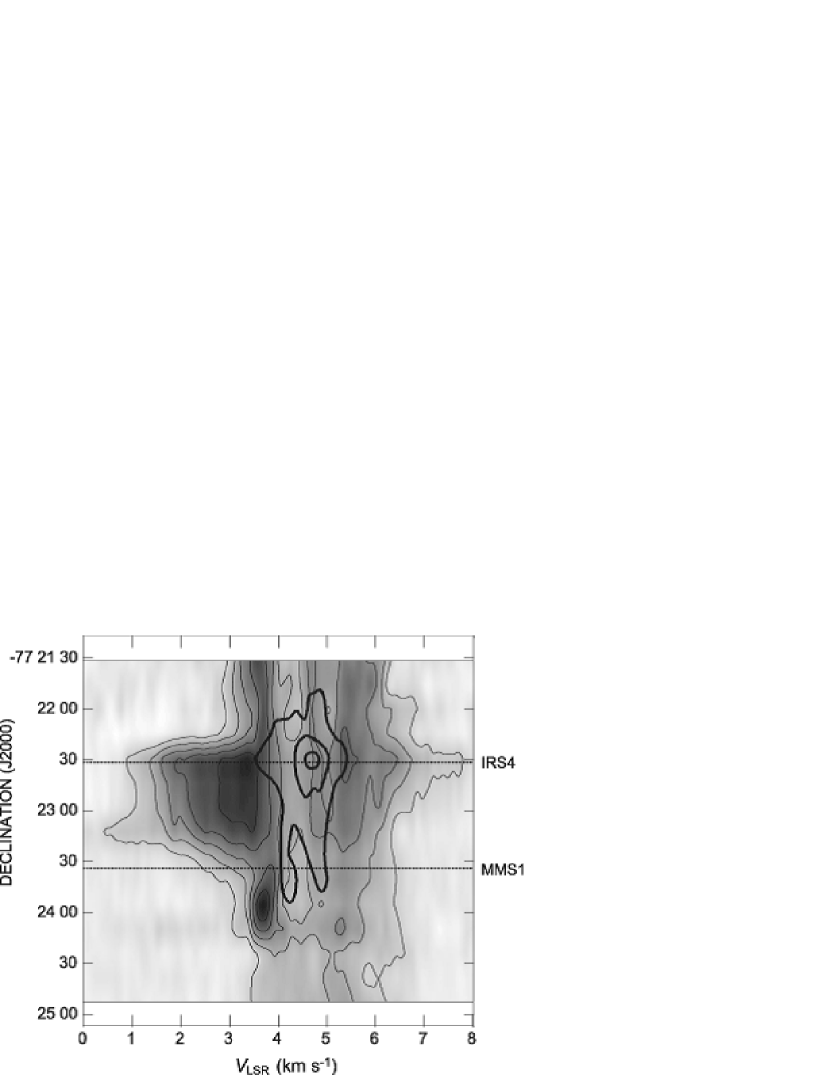
Figure 6: Same as Fig. 5, but for line (b) in Fig. 3.

Around MMS1, there are no conspicuous wide lines (Fig.6). This shows that no outflow is associated with MMS1, which is consistent with the lack of centimeter continuum emission from ionized jets (Lehtinen et al., 2003). Thus, MMS1 is rejected as a driving source of the outflows seen in CO ($J=1-0$) maps (Mattila et al., 1989; Prusti et al., 1991) as well as a launcher of HH49/50.

There are some literatures which summarized properties of class 0 objects (Gregersen et al., 1997; Mardones et al., 1997; Gregersen et al., 2000; Froebrich, 2005). We performed a literature survey about three aspects of the class 0 objects: centimeter continuum emission, CO outflows, and HH objects. All class 0 sources that appeared in the four papers had at least one aspect out of the three. On the other hand, MMS1 has no outflow, centimeter continuum emission, or HH objects. Our results show no evidence of protostar activity in MMS1.

The H¹³CO⁺($J$=4-3) line was detected toward MMS1. The width of the line, 0.36 km s^-1, is smaller than that of the same line toward IRS4. This optically thin line could reflect the cold innermost region of MMS1; thus, the narrow line shows there are no protostars formed yet in MMS1.

The virial mass of MMS1 is derived from the H¹³CO⁺ line width. Assuming the diameter of MMS1 is $40^{\prime\prime}=0.03$ pc (Reipurth et al., 1996), the virial mass is calculated to be 0.49 $M_{\sun}$. This is comparable to the mass (0.45 $M_{\sun}$) derived by Lehtinen et al. (2001) from 1.3 mm continuum observation.

3.3.3 Ced110 IRS6

IRS6 is a binary source (IRS6a and IRS6b), and the near-IR luminosity of IRS6a is a factor of 7 higher than the companion (Persi et al., 2001). This fact indicates that the features obtained toward the binary system mainly derive from IRS6a.

Toward IRS6, we found a weak outflow component in the CO line (Fig.1, 5, and 7c) which has not been detected in past radio observations. The redshifted component extends north, while the blueshifted component is tightly associated with IRS6. The kinematics of the outflow is described in §4.2.

We marginally detected a weak HCO⁺ line toward IRS6 (Fig.7c). In Fig.4 and 5, the IRS6 system does not seem to be surrounded by an extended HCO⁺ envelope. This result supports previous study by Henning et al. (1993) that IRS6 has no massive circumstellar envelope. The small envelope and high $T_{\rm bol}$ of 270 K suggest IRS6 is a relatively evolved protostar.

3.3.4 Ced110 IRS11

Toward IRS11, no high-velocity components were detected by either CO($J$=3-2) or HCO⁺($J$=4-3) lines. A small dense gas envelope associated with this object is detected with the HCO⁺ line (Fig.3, 4, and 5). The radius of the envelope appearing in Fig.5 is about 20^′′, which corresponds to 1.6 $\times 10^{-2}$ pc at the distance of the Cha I dark cloud.

3.3.5 NIR89 and Class II/III Sources

Though NIR89 is classified as a potential class I (Persi et al., 2001), no CO($J$=3-2) outflow was detected (Fig.7e). In addition, no HCO⁺($J$=4-3) emission was detected toward the source. Because this object is thought of as a ”good candidate young brown dwarf” with a stellar mass of 0.02 $M_{\sun}$ (Persi et al., 2001), the amount of the envelope associated with NIR89 should be too small to be detected by our HCO⁺ observations.

No CO outflow components or HCO⁺ emission were detected toward the class II/III objects, ISO-Cha I 97, ISO-ChaI101, and Ced110 IRS2 (Fig.7f - h). This lack of outflow is common among T Tauri stars in general. For HCO⁺ emission, van Zadelhoff et al. (2001) detected the line toward classical T Tauri star LkCa 15 in the Taurus region with a peak $T_{\rm mb}$ of 0.14 K using the James Clerk Maxwell Telescope. Although the line intensity could vary depending on the inclination of the circumstellar disks, in the case of class II/III objects, it is still plausible that we could not detect the HCO⁺ line toward those samples in our observations with 0.15 K sensitivity ($1\sigma$).

4 DISCUSSION

4.1 Molecular Abundance in Envelopes

In dense, cold gas envelopes of protostars and prestellar cores, molecules often freeze out onto dust grains (see e.g. J$\rm{\o}$rgensen et al., 2005). On the other hand, the abundance of some species like HCO⁺ are known to be enhanced in outflows (Rawlings et al., 2004).

We examined the abundance of HCO⁺ toward MMS1 and IRS4 by means of our H¹³CO⁺ ($J=4-3$) observations and 1.3 mm continuum observations (Henning et al., 1993; Reipurth et al., 1996). Assuming that the dust emission is optically thin, the column density of the H₂ molecule, $N$(H₂), is calculated with

$$N({\rm H}_{2})={{S^{\rm beam}_{\nu}}\over\Omega_{\rm beam}\mu m_{\rm H}\kappa_{\nu}B_{\nu}(T_{\rm D})},$$ (1)

where $S^{\rm beam}_{\nu}$ is the 1.3 mm flux density per beam, $\Omega_{\rm beam}$ is the beam solid angle, $\mu=2.3$ is the mean molecular weight, $m_{\rm H}$ is the mass of the H atom, $\kappa_{\rm 1.3mm}$ is the mass absorption coefficient per gram, and $B_{\nu}(T_{\rm D})$ is the Planck function at the dust temperature $T_{\rm D}$. We employed $\kappa_{\rm 1.3mm}=0.01$ cm² g^-1 for IRS4, which is the recommended value for very dense regions (Ossenkopf & Henning, 1994). Meanwhile, we applied the value of 0.005 cm² g^-1 for MMS1, which is the adopted value for prestellar core L1689B (Andr$\rm{\grave{e}}$ et al., 1996). The substituted values of $S^{\rm beam}_{\nu}$ are 370 mJy for MMS1 (Reipurth et al., 1996) and 101 mJy for IRS4 (Henning et al., 1993). We employed a dust temperature of 20 and 21 K for MMS1 and IRS4, respectively, based on Lehtinen et al. (2001). The resulting H₂ column density is $2.2\times 10^{23}$ cm^-2 for MMS1 and $2.8\times 10^{22}$ cm^-2 for IRS4.

We also calculated the column density of H¹³CO⁺ under LTE conditions and the assumption that the excitation temperature equals the dust temperature. Comparing $N$(H₂) obtained from dust observations with $N$(H¹³CO⁺), we estimated the abundance of HCO⁺ to be $X$(HCO⁺) = $2.6\times 10^{-10}$ for MMS1 and $3.4\times 10^{-9}$ for IRS4. We set the isotropy ratio of [H¹³CO⁺]/[HCO⁺] = 70. The results are summarized in Table ASTE Submillimeter Observations of a Young Stellar Object Condensation in Cederblad 110.

J$\rm{\o}$rgensen et al. (2004) reported average $X$(HCO⁺) $=8.0\times 10^{-10}$ for prestellar cores and $1.1\times 10^{-8}$ for class I sources. J$\rm{\o}$rgensen et al. (2005) pointed out that the molecular depletion in envelopes of class I objects is less significant because of heating by their central sources. Furthermore, Rawlings et al. (2004) reported that the abundance of HCO⁺ is enhanced in molecular outflows. Our results are not in contradiction with abundances reported in similar objects. However, it is not appropriate to investigate the results in more detail, because the mass absorption coefficient $\kappa$ and the LTE approximation have large uncertainties. $\kappa$ has different values depending on dust size, shape, structure, and so on (Henning et al., 1995). In addition, Mennella et al. (1998) show $\kappa$ has a dependence on temperature.

4.2 Gas Infall toward the Protostars

We show HCO⁺($J$=4-3) line profiles toward four class I sources in Fig. 7a, c, d and e. None of the profiles show the blue asymmetry which is one of the indicators of infalling gas toward protostars (Leung & Brown, 1977; Zhou, 1992). In a simplified model of an infalling envelope, the blueshifted line component is stronger than the redshifted component. This is because the redshifted component is absorbed by the cooler infalling material in the near half of the envelope along the line of sight. Do our results mean these objects have no infalling gas?

As mentioned in the previous sections, IRS4 and IRS6 obviously have outflows. This is clear evidence of the existence of infalling gas toward the protostars. Gregersen et al. (1997, 2000) have revealed that blue asymmetry line profiles do not appear in about half of class 0 and I sources, although they are thought to be in the active accretion phase.

Some reasons are suggested why blue asymmetry does not appear in all sources. One great problem is confusion with outflows. If a redshifted outflow exists in the telescope beam, the redshifted line components absorbed by the infalling envelope would be compensated. It is also difficult to separate the influence of other velocity components such as circumstellar disks and ambient gas in observations with a large beam of single dish radio telescopes. In our observations, as an example, a wing component is detected in the CO line profile toward IRS4. This profile obviously shows that our 22^′′ beam covers the outflowing component. In general, there are some possibilities to confuse not only outflow, but core rotation and other large-scale physical structures with infall, all of which affect obtained line profiles. Thus, it is difficult to investigate infall motion in targeted observations toward protostars without high-resolution spatial information about the envelope.

The other problem is optical depth. Choosing molecular lines with appropriate optical depth is necessary to detect infall motion of the inner portion of the envelope in general, not only for Ced110. When a protostar is highly embedded in a dense clump and an observed line becomes optically too thick, the line cannot convey information of the inner infalling region any more and reflects only properties of foreground components.

4.3 Kinematics of Outflows

We calculated the physical parameters of the outflows from IRS4 according to the procedures of Choi et al. (1993). In these procedures, the CO column density for each channel in units of cm^-2, $N^{\rm CO}_{i}$, and the mass per channel, $M_{i}$, are calculated from

$$N^{\rm CO}_{i} = 1.10\times 10^{15}{T_{\rm R3-2}\Delta V\over D(n,T_{\rm K})}{\tau_{32}\over 1-\exp(-\tau_{32})},$$ (2)

$$M_{i} = \mu m_{{\rm H}_{2}}d^{2}\Omega N^{\rm CO}_{i}{[{\rm H}]\over[{\rm C}]}{[{\rm C}]\over[{\rm CO}]},$$ (3)

where

$$D(n,T_{\rm K})=f_{2}[J_{\nu}(T_{\rm ex})-J_{\nu}(T_{\rm bk})][1-\exp(-16.597/T_{\rm ex})],$$ (4)

$T_{\rm R3-2}$ is the line intensity of the CO($J$=3-2) line, $\Delta V$ is the channel width in km s^-1, $f_{2}$ is the fraction of CO molecules in the $J=2$ state, $d$ = 160 pc is the distance to the Cha I cloud, $\Omega$ is the solid angle subtended by emission, [H]/[C]$=2.5\times 10^{3}$, [C]/[CO] $=8$, and $\tau_{32}$ is the optical depth of the line. We calculated $\tau_{32}\sim 0.4$ comparing with CO($J$=3-2) and CO($J$=1-0) line-wing intensity (Prusti et al., 1991). In this calculation, we assumed that the excitation temperatures $T_{\rm ex}$ of the two lines are equal to 20 K. According to large velocity gradiant simulations by Choi et al. (1993), $D(n,T_{\rm K})$ does not vary so much within the reasonable density and temperature range. Therefore, we set the same value of $D(n,T_{\rm K})=1.5$ as in Choi et al. (1993). The mass $M$, momentum $P$, and kinetic energy $E_{\rm k}$ can be estimated from

$$M = \Sigma_{i}M_{i},$$ (5)

$$P = \Sigma_{i}M_{i}|V_{i}-V_{0}|,$$ (6)

$$E_{\rm K} = \Sigma_{i}{1\over 2}M_{i}(V_{i}-V_{0})^{2},$$ (7)

where $V_{0}$ is the system velocity. We also calculated the dynamical timescale $t_{\rm d}=R/V_{\rm ch}$ where the characteristic velocity $V_{\rm ch}=P/M$, mass loss rate $\dot{M}=M/t_{\rm d}$, and average driving force $F=P/t_{\rm d}$.

The results are shown in Table 6. We adopted an inclination of the outflow axis from the line of sight of $i=72\arcdeg$ (Pontoppidan & Dullemond, 2005). They derived this value through comparing near-IR images with three-dimensional Monte Carlo radiative transfer code of a disk-shadow projection model. This value is consistent with the fact that the high-resolution infrared images (Zinnecker et al., 1999; Persi et al., 2001) clearly show the edge-on disklike silhouette of IRS4.

We compared the derived values with those in a statistical study of outflows (Wu et al., 2004) in which they show a correlation between the mass, $L_{\rm bol}$ and $F$ for 391 samples. The mass of IRS4’s blueshifted outflow is smaller by about 1 order of magnitude than the average of the same $L_{\rm bol}$ sources in Wu et al. (2004), but it is still within the range of variation of the data.

In contrast, the derived mass loss rate is rather large in IRS4 despite its small size. Generally, the mass loss rate by jets is about 1% and that by outflows is10 % of the mass accretion rate (Hartigan et al., 1995). The derived value of 1.1 $\times 10^{-6}M_{\sun}$ yr^-1 is comparable to the typical accretion rate for protostars, 10${}^{-6}M_{\sun}$ yr^-1, derived by the similarity solution for thermally supported clouds with 10 K (Hartmann, 1998).

HH49/50 is a group of knots located 10.5$\arcmin$ southwest of the Ced110 region. Studies of radial velocity and proper motion (Schwartz & Dopita, 1980; Schwartz et al., 1984) revealed the knots move toward the southwest and away from us. Mattila et al. (1989) and Prusti et al. (1991) identified Ced110 IRS4 as the driving source of these HH objects judging from their CO outflow map, because they found a diffuse redshifted component that extends in the southwest of IRS4 and the alignment of knots is almost parallel to the direction to IRS4. In our observations, we detected two components that extend to the south of IRS4. One is the prominent blueshifted outflow which has an opposite line-of-sight direction of movement from HH objects. The other is the diffuse redshifted component that appeared in Fig.2. This complicated morphology makes it difficult to discuss the relation between IRS4 and HH49/50. To resolve this issue, one should enlarge CO observations toward the southwest to know the larger structure of the outflow.

In Fig.5 and 6, the HCO⁺ line toward IRS4 indicates a wide profile as well as a CO line. Infalling and outflowing gas seem to be the causes of this wide line (Gregersen et al., 1997; Masunaga & Inutsuka, 2000), and perhaps, both the effects are blended. In both position-velocity diagrams, the blueshifted component of the HCO⁺ line is broader than redshifted component. This is identical to the tendency of CO outflow, which indicates the wide HCO⁺ line is mainly caused by the outflow. As in the HCO⁺ channel map (Fig.4), the blueshifted component extends to the west of IRS4, whereas redshifted component is elongated to the north. This aspect again corresponds with the morphology of the CO outflow (Fig.2).

Another method to use to determine what makes the wide line profile is to compare the velocity of infalling and outflowing gas. We calculated the free fall velocity of infalling gas, $v_{\rm ff}=0.31$ – 0.56 km s^-1, assuming the mass range of 0.10 – 0.32 $M_{\sun}$ derived by Persi et al. (2001), and a diameter of the envelope of $1.7\times 10^{-2}$ pc. These $v_{\rm ff}$ are smaller than the line width, which indicates the outflow has a larger contribution to the wide line profiles.

Toward IRS6, we derived some physical parameters of the outflow in the same procedure as for IRS4 and show the result in Table. 6. In the case of IRS6, we could not correct the effect of the inclination of the outflow axis because of a lack of information. Besides, there have been no CO($J$=1-0) observations toward IRS6 in previous years, so we could not derive $\tau_{32}$. Here we use the same $\tau_{32}$ as toward IRS4. Although there are ambiguities of inclination and optical depth, the outflow from IRS6 is more than 1 order of magnitude smaller than that from IRS4. This is consistent with our estimation of its evolved status with a small envelope. This interpretation is not consistent with the young age of the outflow; however, when the outflow is nearly in pole-on configuration, the dynamical timescale of the outflow will be calculated to be smaller than the true value. We need to know the inclination angle of this source to correct this mismatch.

4.4 Interaction between Cha-MMS1 and the Outflow from IRS4

Figure 1 shows the blueshifted component of the outflow from the IRS4 has negative spatial correlation with the continuum emission from Cha-MMS1. The outflow seems to change its direction at the edge of the MMS1. In Fig.2, the outflow component with the highest velocity is distributed at the midpoint between IRS4 and MMS1. In addition, the velocity of the outflow suddenly declines in front of MMS1 (Fig.6), i.e., the flow seems to be decelerated by MMS1. Do these characteristics indicate that MMS1 interacts with the outflow from IRS4?

There were no emissions detected from shock tracer molecules in submillimeter wavelength in our observations. However, considering IRS4’s low luminosity ($L_{\rm bol}=1.0L_{\odot}$; Lehtinen et al., 2001), weak outflow properties, and high upper energy levels of $>70$ K, it is conceivable that the outflow-core interaction could not increase the temperature enough to excite these molecules. We could not rule out that a weak interaction does occur. Kontinen et al. (2000) pointed out that outflows and radiation from the neighboring young stars have prospects for influencing the chemical processes in MMS1. Here we considered the impact of the interaction from following two view-points.

First we investigate momentum. Here we compare the momentum brought by the outflow with gas momentum in MMS1. When an outflow with density $\rho$ and velocity $v$ is colliding with a surface of radius $r$ for a time duration $t$, we can obtain the mass $\dot{M}_{\rm col}$ colliding in a unit of time and the momentum $P_{\rm outflow}$ as,

$$P_{\rm outflow}=\dot{M}_{\rm col}vt=\pi r^{2}v^{2}\rho t.$$ (8)

Now we estimate the density of the outflow. For simplicity, we assume the outflow has a cone shape with a base diameter of 40^′′ (= 3.1 $\times 10^{-2}$ pc) and a height of 60^′′ (= 4.7 $\times 10^{-2}$ pc) judging from Fig.1. Calculating the density $\rho$ of the outflow from this assumption with the derived mass, we obtain $\rho=6.5\times 10^{-20}$ g cm^-3. Assigning this density, radius $r=1.6\times 10^{-2}$ pc and $t$ which equals the dynamical timescale of the flow ($1.0\times 10^{4}$ yr) to equation (8), we derived a momentum of 0.88 $M_{\sun}$ km s^-1. Meanwhile, the momentum of gas in MMS1 is calculated to be $P_{\rm MMS1}=0.15$ $M_{\sun}$ km s^-1 from the mass of 0.45 $M_{\sun}$ and the velocity of 0.34 km s^-1 derived from the H¹³CO⁺ line profile, which is a combination of turbulence and thermal width, removing the contribution of the spectral resolution. As a result, $P_{\rm outflow}$ is much larger than $P_{\rm MMS1}$, which means the motion of the gas in MMS1 is easily affected when the outflow collide with the core.

Although the MMS1 contours in Reipurth et al. (1996) have an asymmetry, it is difficult to confirm the collisional impact on the geometry of MMS1 with their map. But in our HCO⁺ position-velocity diagram (Fig.6), we could find the sign of the kinematic motion of the outer gas of MMS1 caused by the collision. The dip in the northern side of MMS1 is slightly ($\sim$ 0.3 km s^-1) blueshifted, which results in the velocity gradient on the map. This gradient is consistent with the IRS4 outflow direction. Precise calculations of the momentum for this gradient is difficult with our data set, but in a rough upper limit estimation, the momentum for making this dip velocity gradient, $P_{\rm grad}$, should be less than the product of the velocity difference and the whole mass of MMS1, $P_{\rm grad}<0.14M_{\odot}$ km s^-1. The momentum provided by the outflow is larger than $P_{\rm grad}$; thus, this outer gas motion could be excited by the interactions with the outflow.

The other point of discussion is the time scale before induced star formation is triggered in MMS1. One example of outflow-triggered star formation is L1551 NE in Taurus (Yokogawa et al., 2003). In the case of MMS1, before star formation is triggered, it is necessary that a rise in pressure outside of MMS1 by colliding with the outflow reaches the center of the core. The velocity of this propagation equals the sound speed, or the shock speed if a shock has been excited. The sound speed under 10 K is 0.19 km s^-1. With this velocity, the signal of the collision arrives at the center in $7.2\times 10^{4}$ yr. This is about an order of magnitude longer than the dynamical timescale of the outflow. Under this condition, triggered star formation would not have occurred yet. Next, we also consider the case in which a shock exists. In order to derive the shock speed, we need to know the density structure around MMS1, because the shock speed depends on the difference between inner and outer density of MMS1. According to Reipurth et al. (1996), the difference between the 1.3 mm continuum intensity at the center and outside of the MMS1 is about a factor of 2. Under optically thin conditiona, the difference of the intensity is identical to that of density, and the shock speed equals half of the outflow speed, 5.3 km s^-1. With this speed, the shock would arrive at the center in $2.8\times 10^{3}$ yr from the point of the collision. Considering the time to reach the boundary of MMS1 from its departure from IRS4, the time for the outflow to arrive at the center of MMS1 is $8.5\times 10^{3}$ yr, about the same as the dynamical timescale of the outflow. If the estimate of density structure is correct, compression has just reached to the center of MMS1 and collapse would just be triggered. Considering that we could not detect any infall and outflow signature around the source, it is possible that MMS1 is in a very young stage of its evolution.

5 SUMMARY

We observed an YSO condensation in the Cederblad 110 region of the Chamaeleon I dark cloud by CO($J$=3-2), HCO⁺($J$=4-3), H¹³CO⁺($J$=4-3), CH₃OH($J$=$7_{K}$-$6_{K}$), SO($J$=$8_{9}$-$7_{8}$), and SiO($J$=8-7) submillimeter lines with the ASTE 10m telescope. Results are as follows.

1) We found a dense HCO⁺ clump. This clump is an aggregate made up of three components associated with IRS4, IRS11, and Cha-MMS1. Although these sub-components do not appear in the integrated intensity map, we can distinguish them in the channel map and the position-velocity diagrams.

2) We detected CO ($J=3-2$) outflow components around IRS4 and IRS6, but not around Cha-MMS1, IRS11, or NIR89. Our observations with high angular resolution show the outflows previously known in this region are launched by IRS4, not by MMS1. This result suggests MMS1 is not a protostar but still in the prestellar phase.

3) Each HCO⁺($J$=4-3) line profile toward IRS4, IRS11, and MMS1 all have ”red” asymmetry instead of blue asymmetry, which is a marker of infalling gas. However, our result does not necessarily mean there is no infall in these young sources, because the outflows from IRS4 and IRS6 are direct evidences of gas infall.

4) The blue-shifted outflow from IRS4 seems to collide against MMS1. The outflow veers and the velocity declines just in front of MMS1. Though emission lines from shock tracer molecules such as CH₃OH, SO, and SiO are not detected, it is plausible because the outflow from IRS4 is rather weak for excitation of these molecules.

5) Momentum calculations show the outflow from IRS4 is strong enough to affect gas motion in MMS1, although the outflow is so young that the star formation process has not been triggered yet, or has just been triggered. This is consistent with the very young status of MMS1 and the lack of any outflows, jets, and masers.

Table 1: YSOs in Cederblad 110 Region

Name	R.A. (J2000)	Dec. (J2000)	IR class	$T_{\rm bol}$	$L_{\rm bol}$	References
Cha-MMS1	11 06 31.7	-77 23 32	0	20	0.46	1
			0	36	0.38	2
Ced110 IRS4	11 06 47.1	-77 22 34	I	72	1.0	1
			0/I	59	1.0	2
Ced110 IRS6a	11 07 9.8	-77 23 05	I	260	0.8	1
Ced110 IRS11	11 06 58.8	-77 22 50	I	$\cdots$	0.17	3
NIR89	11 06 53.8	-77 24 00	I	$\cdots$	$\cdots$
ISO-Cha I 97	11 07 17.0	-77 23 08	II	$\cdots$	$\cdots$
ISO-Cha I 101	11 07 21.7	-77 22 12	II	$\cdots$	$\cdots$
Ced110 IRS2	11 06 16.8	-77 21 55	III	2700	3.4	1

References. — (1) Lehtinen et al. (2001); (2) Froebrich (2005); (3) Persi et al. (2001)

Table 2: CO($J$=3-2) Observations on YSOs

	$T_{\rm MB}$	$\int T_{\rm MB}{\rm d}v$
	(K)	(K km s-1)
Cha MMS1	6.94 $\pm$ 0.21	14.4 $\pm$ 0.1
Ced110 IRS4	8.39 $\pm$ 0.43	34.7 $\pm$ 0.1
Ced110 IRS6	11.37 $\pm$ 0.20	24.3 $\pm$ 0.1
Ced110 IRS11	6.50 $\pm$ 0.47	15.5 $\pm$ 0.1
NIR89	7.86 $\pm$ 0.41	17.6 $\pm$ 0.1
ISO-ChaI 97	8.22 $\pm$ 0.21	16.0 $\pm$ 0.1
ISO-ChaI 101	6.94 $\pm$ 0.27	14.1 $\pm$ 0.1
Ced110 IRS2	7.80 $\pm$ 0.38	14.9 $\pm$ 0.1

Table 3: HCO⁺($J$=4-3) Observations on YSOs

	$T_{\rm MB}$	$V_{\rm LSR}$	$\Delta V$	$\int T_{\rm MB}{\rm d}v$
	(K)	(km s-1)	(km s-1)	(K km s-1)
Cha MMS1	1.64 $\pm$ 0.09	4.49 $\pm$ 0.12	0.68 $\pm$ 0.14	1.11 $\pm$ 0.01
Ced110 IRS4	3.00 $\pm$ 0.09	4.46 $\pm$ 0.13	1.55 $\pm$ 0.15	4.58 $\pm$ 0.01
Ced110 IRS6	0.65 $\pm$ 0.09	4.62 $\pm$ 0.18	1.53 $\pm$ 0.28	0.73 $\pm$ 0.01
Ced110 IRS11	1.47 $\pm$ 0.08	4.67 $\pm$ 0.13	0.90 $\pm$ 0.15	1.35 $\pm$ 0.01
NIR89	$<$ 0.16	$\cdots$	$\cdots$	$<$ 0.35
ISO-ChaI 97	$<$ 0.17	$\cdots$	$\cdots$	$<$ 0.70
ISO-ChaI 101	$<$ 0.36	$\cdots$	$\cdots$	$<$ 0.54
Ced110 IRS2	$<$ 0.29	$\cdots$	$\cdots$	$<$ 0.30

Table 4: H¹³CO⁺($J$=4-3) Observations on YSOs

	$T_{\rm MB}$	$V_{\rm LSR}$	$\Delta V$	$\int T_{\rm MB}{\rm d}v$
	(K)	(km s-1)	(km s-1)	(K km s-1)
Cha MMS1	0.26 $\pm$ 0.03	4.63 $\pm$ 0.13	0.36 $\pm$ 0.16	0.11 $\pm$ 0.01
Ced110 IRS4	0.13 $\pm$ 0.03	4.53 $\pm$ 0.18	1.72 $\pm$ 0.29	0.18 $\pm$ 0.01

Table 5: H₂ Column Density and HCO⁺ Abundance toward IRS4 and MMS1

	$S^{\rm beam}_{\rm 1.3mm}$	$T_{\rm D}$	$N$(H2)	$X$(HCO+)
	(mJy)	(K)	(cm-2)
Cha MMS1	370	20	$2.2\times 10^{23}$	$2.6\times 10^{-10}$
Ced110 IRS4	101	21	$2.8\times 10^{22}$	$3.4\times 10^{-9}$

References. — (1) Reipurth et al. (1996); (2) Henning et al. (1993); (3) Lehtinen et al. (2001)

Table 6: Parameters for Outflows from Ced 110 IRS4 and IRS6

	$R_{\rm outflow}$	$M$	$t_{\rm d}$	$\dot{M}$	$P$	$E_{k}$	$F$
	(pc)	($M_{\sun}$)	(year)	($M_{\sun}$yr-1)	($M_{\sun}$km s-1)	($M_{\sun}$(km s-1)2)	($M_{\sun}$ km s-1 yr-1)
IRS4
Blue	6.5$\times 10^{-2}$	1.1$\times 10^{-2}$	1.0$\times 10^{4}$	1.1$\times 10^{-6}$	7.1$\times 10^{-2}$	2.4$\times 10^{-1}$	7.1 $\times 10^{-6}$
Red	2.5$\times 10^{-2}$	9.8$\times 10^{-4}$	2.9$\times 10^{3}$	3.4$\times 10^{-7}$	7.7$\times 10^{-3}$	3.1$\times 10^{-2}$	2.7 $\times 10^{-6}$
IRS6
Blue	1.6$\times 10^{-2}$	$3.3\times 10^{-4}$	7.8$\times 10^{3}$	4.3$\times 10^{-8}$	6.5$\times 10^{-4}$	6.7$\times 10^{-4}$	8.4 $\times 10^{-8}$
Red	3.1$\times 10^{-2}$	$5.7\times 10^{-4}$	1.3$\times 10^{4}$	4.3$\times 10^{-8}$	1.3$\times 10^{-3}$	1.5$\times 10^{-3}$	9.9 $\times 10^{-8}$

References

- Andr et al. (1996) Andr P., Ward-Thompson D., & Motte F. 1996, A&A, 314, 625
- Arce & Goodman (2002) Arce H. G., & Goodman A. A. 2002, ApJ, 575, 911
- Bachiller (1996) Bachiller R. 1996, ARAA, 34, 111
- Bally et al. (2006) Bally J., Walawender J., Luhman K. L., & Fazio G. 2006, ApJ, 132, 1923
- Cederblad (1946) Cederblad S. 1946, Lund Medd. Astron. Obs. Ser. II, 119, 1
- Choi et al. (1993) Choi M. H., Evans II N., J., & Jaffe D. T. 1993, ApJ, 417, 624
- Evans (1999) Evans II N. J. 1999, ARA&A, 37, 311
- Ezawa et al. (2004) Ezawa H., Kawabe R., Kohno K., & Yamamoto S. 2004, Proc. SPIE, 5489, 763
- Froebrich (2005) Froebrich D. 2005, ApJS, 156, 169
- Gregersen et al. (1997) Gregersen E. M., Evans N. J., Zhou S., & Choi M. 1997, ApJ, 484, 1997
- Gregersen et al. (2000) Gregersen E. M., Evans N. J., Mardones D., & Myers P. C. 2000, ApJ, 533, 440
- Haikala et al. (2005) Haikala L. K., Harju J., Mattila K., & Toriseva M. 2005, A&A, 431, 149
- Hartigan et al. (1995) Hartigan P., Edwards S., & Ghandor L., 1995 ApJ, 452, 736
- Hartmann (1998) Hartmann L. 1998, Accretion Processes in Star Formation (Cambridge: Cambridge University Press)
- Henning et al. (1995) Henning Th., Michel B., Stognienko R. 1995 P&SS, 43, 1333
- Henning et al. (1993) Henning Th., Pfau P., Zinnecker H., & Prusti T. 1993, A&A, 276, 129
- Jrgensen et al. (2004) Jrgensen, J. K., Schier F. L., & van Dishoeck E.F. 2004, A&A, 416, 603
- Jrgensen et al. (2005) Jrgensen, J. K., Schier F. L., & van Dishoeck E.F. 2005, A&A, 435, 177
- Kamazaki et al. (2005) Kamazaki T., et al. 2005, Astronomical Society of the Pacific Conference Series, 347, 533
- Kontinen et al. (2000) Kontinen S., Harju J., Heikkilä A., & Haikala L. K. 2000, A&A, 361, 704
- Kutner & Ulich (1981) Kutner, M., & Ulich, B. L. 1981, ApJ, 250, 341
- Lada & Lada (2003) Lada C. J.,& Lada E. A. 2003, ARA&A, 41, 57
- Lehtinen et al. (2001) Lehtinen K., Haikala L. K., Mattila K., & Lemke D. 2001, A&A, 367, 311
- Lehtinen et al. (2003) Lehtinen K., Harju J., Kontinen S., & Higdon J. L. 2003, A&A, 401, 1017
- Leung & Brown (1977) Leung C. M., & Brown R. L. 1977, ApJ, 214, L73
- Mardones et al. (1997) Mardones D, Myers P. C., Taffala M.,Wilner D. J.,Bachiller R., & Garay G. 1997, ApJ 489, 719
- Masunaga & Inutsuka (2000) Masunaga H., & Inutsuka S. 2000, ApJ, 536, 406
- Matsuo et al. (1998) Matsuo M., Sakamoto A., & Matsushita A. 1998, PASJ 50, 359
- Mattila et al. (1989) Mattila K., Liljestrom T., & Toriseva M. 1989, in ESO Conf. Proc., 33, Low Mass Star Formation and Pre-Main Sequence Objects, ed. B. Reipurth, 153
- Matzner & McKee (2000) Matzner C. D, & McKee C. F. 2000, ApJ, 545, 364
- Mennella et al. (1998) Mennella V., Brucato J. R., Colangeli L., Palumbo P.,Rotundi A., & Bussoletti E. 1998, ApJ, 496, 1058
- Mizuno et al. (1994) Mizuno A., Onishi T., Hayashi M., Ohashi N., Sunada K., Hasegawa T., & Fukui, Y. 1994, Nature, 368, 719
- Myers & Ladd (1993) Myers P. C., & Ladd E. F. 1993, ApJ, 413, L47
- Nakano et al. (1995) Nakano T., Hasegawa T., & Norman C. 1995, ApJ, 450, 183
- Ossenkopf & Henning (1994) Ossenkopf V., & Henning Th. 1994, A&A, 291, 943
- Persi et al. (2000) Persi P., et al. 2000, A&A, 357, 219
- Persi et al. (2001) Persi P., Marenzi A. R., Gómez M., & Olofsson G. 2001, A&A, 376, 907
- Pontoppidan & Dullemond (2005) Pontoppidan K. M., & Dullemond C. P. 2005, A&A, 435, 595
- Prusti et al. (1991) Prusti T., Clark F. O., Whittet D. C. B., Laureijs R. J., & Zhang. C. Y. 1991, MNRAS, 251, 303
- Rawlings et al. (2004) Rawlings J. M. C., Redman M. P., Keto E., & Williams D. A. 2004, MNRAS, 351, 1054
- Reipurth et al. (1996) Reipurth B., Nyman L.- ., & Chini R. 1996, A&A, 314, 258
- Schwartz & Dopita (1980) Schwartz R., & Dopita M. A. 1980, ApJ, 236, 543
- Schwartz et al. (1984) Schwartz R., Jones B.-F., & Sirk M. 1984, AJ, 89, 1735
- Takakuwa et al. (2003) Takakuwa S., Ohashi N., & Hirano N. 2003, ApJ, 590, 932
- Wang et al. (1994) Wang Y., Jaffe D. T., Graf U. U., & Evans N. J. 1994, ApJS, 95, 503
- Whittet et al. (1997) Whittet D. C. B., Prusti T., Franco G. A. P., Gerakines P. A., Larson K. A., & Wesselius P. R. 1997, A&A, 327, 1194
- Wu et al. (2004) Wu Y., Wei Y., Zhao M., Shi Y., Yu W., Qin S., & Huang M. 2004, A&A, 426, 503
- Yokogawa et al. (2003) Yokogawa S., Kitamura Y., Momose M., & Kawabe R. 2003, ApJ, 595, 266
- van Zadelhoff et al. (2001) van Zadelhoff G.-J., van Dishoeck E. F., Thi W.-F., & Blake G. A. 2001, A&A, 377, 566
- Zhou (1992) Zhou S. 1992, A&A, 394, 204
- Zinnecker et al. (1999) Zinnecker H., et al. 1999, A&A, 352, L73