Upper and lower bounds for the large polaron dispersion in $D=1,2,3$ dimensions

Abstract

Numerical results for the polaron dispersion are presented for an arbitrary number of space dimensions. Upper and lower bounds are calculated for the dispersion curves. They are rather close to each other in the cases of small electron-phonon couplings usual for real polar materials. To describe the dispersion in other materials, we suggest a simple fitting formula which can be applied at intermediate values of the Fröhlich electron-phonon coupling constant. Its validity is approved by the comparison with direct calculations and previously obtained results. This makes our results not only reliable and highly accurate but also easy reproducible.

I Introduction

The electron-phonon interaction influences the properties of charge carriers (electrons) in polar semiconductors or ionic crystals. An electron polarizes a medium and, being surrounded by a cloud of virtual phonons, is captured by a self-induced potential which can move in a material. Such a quasiparticle is called a polaron. The larger the value of the Fröhlich electron-phonon coupling constant $\alpha$, the more pronounced are polaron effects. In particular, the electron-phonon interaction results in an electron binding energy, in a renormalization of its mass and in a nonparabolic energy-momentum dependence.

In the present paper, we study the large polaron dispersion law that is the dependence of the polaron ground-state energy $E(\alpha,Q)$ on the total polaron momentum $Q$. The technological progress in man-made structures has caused a rapidly increasing literature on systems of reduced dimensionality, in particular, on the effects of electron-phonon interaction in quantum wells, wires and dots. Thus, the dimensionality $D$ of space in our study may be different: $D=1,2,3$.

Here and in what follows all quantities are dimensionless, the energy, mass and length units being $\hbar\omega$, $m$ and $\sqrt{\hbar/2m\omega}$, respectively, where $\omega$ is the longitudal optical (LO) phonon frequency and $m$ is the free electron band mass. For instance, the polaron kinetic energy $P^{2}/2m_{pol}$ at small momentum $P$ is written down as $Q^{2}/m(\alpha)$ in our dimensionless units where $m_{pol}$ is the polaron effective mass and $m(\alpha)=m_{pol}/m$.

The literature on polaron is enormous but it concerns mostly the energy $E(\alpha,0)$ of the bulk ($D=3$) polaron at rest. Nevertheless, the first results were obtained on a bulk polaron dispersion law even in a very early paper by Fröhlich, Pelzer and Zienau zienau where the authors used the first order of the Brillouin-Wigner perturbation theory. Later Whitfield and Puff whit suggested an improved version of the polaron energy-momentum relation in the weak-coupling regime. For these and other early papers see also the review article by Appelappel where qualitative considerations on the behavior of the dispersion curve were given. The results obtained demonstrate that the bulk polaron energy-momentum relation is quadratic for small $Q$ but then bends over and becomes horizontal when the energy approaches the continuum edge $E_{c}$ which is reached at some finite value $Q_{c}$ of the polaron momentum. At this momentum the moving polaron energy $E_{c}=E(\alpha,Q_{c})$ exceeds the ground-state energy $E(\alpha,0)$ of the polaron at rest exactly by the energy of a free phonon $\hbar\omega$ (which is just unity in our notation).

Below the continuum edge $E_{c}=E(\alpha,0)+1$ (that is at $Q<Q_{c}$) the ground-state energy $E(\alpha,Q)$ is an isolated and well defined eigenvalue. There are some important rigorous results concerning the properties of the dispersion $E(\alpha,Q)$ (see Ref. lowen ; spohn )

• $E(\alpha,Q)$ is a real analytic function of $\alpha$ and $Q$ for $0\leq\alpha<\infty,Q^{2}\leq 1$. The former constraint on $Q$ can be removed totally for $D=1,2$. For $D=3$ the domain of $Q$ can be extended up to a finite value $Q_{c}$, where the energy reaches the continuum edge.

• $E(\alpha,Q)$ decreases with $\alpha$ and increases with $Q$ below the continuum edge.

• The inequality $E(\alpha,0)<E(\alpha,Q)$ holds for $Q\neq 0$ and $0\leq\alpha<\infty$.

• The upper bound is given by the inequality

  $$E(\alpha,Q)\leq\min[E(\alpha,0)+Q^{2},E(\alpha,0)+1].$$ (1)

The simplest and seemingly the most natural way to describe the dispersion is the first order of the Raleigh-Schrödinger perturbation theory (RSPT). For $D=1,2,3$ it results in the well-known formulae:

$$E(\alpha,Q) = Q^{2}-\alpha{\pi\over 2\sqrt{1-Q^{2}}}\ {\rm for}\ D=1,$$ (2a)

$$E(\alpha,Q) = Q^{2}-\alpha K(Q^{2})\ {\rm for}\ D=2,$$ (2b)

$$E(\alpha,Q) = Q^{2}-\alpha{\arcsin Q\over Q}\ {\rm for}\ D=3.$$ (2c)

Here $K(m)$ is the complete elliptic integral of the first kind.

The results of the RSPT contradict the rigorous properties of the dispersion. For instance, all three functions of Eq. (2) have maxima at some momenta $Q_{m}<1$ so they are decreasing functions in the region $Q_{m}<Q<1$. Moreover, the expressions for $D=1,2$ diverge at $Q=1$, so the RSPT evidently fails to work near this value. At small $Q\ll 1$ RSPT leads however to correct (to the first order in $\alpha$) parabolic functions of the effective mass approximation.

After the above cited paperzienau different variational approaches were developed to calculate the polaron dispersion. The paper by Lee, Low and Pines lee should be mentioned among earlier articles on polarons. For sufficiently large $Q$ their variational result is weaker than the nonanalytical upper bound (1), the dispersion curve intersects the continuum edge and the deviation from the correct result is of the order $\alpha^{0}$, which does not provide the necessary accuracy of calculations.

More advanced variational calculations were performed by Larsenlarsen , and by Warmenbol, Peeters and Devreese warm2 ; warmenbol . These and some other papers will be discussed in more detail later.

Naturally, only upper bounds could be obtained with the variational methods of these papers. It is much more difficult to derive a lower bound, and it was found by Lieb and Yamazaki lieb but only for $Q=0$. The general procedure to obtain the $Q-$dependent lower bound was developed by Gerlach and Kalina gerl3 .

In the present paper, we combine the variational upper bound obtained with the expansion of the trial wave function in numbers of virtual phonons with the lower bound of Ref. gerl3 . In principle, our variational upper bound could lead to exact solutions but in practice we have to cut the expansion and work with an approximation obtained this way. For small values of the electron-phonon coupling constant $\alpha$ which are common for most of the polar materials the corridor between these two estimates is very narrow, so that we can pretend to finding numerically exact solutions.

The lower bound gives too poor results for intermediate values $\alpha\sim 1$. Besides the huge numerical job does not allow us to reach the necessary accuracy with the upper bound. To overcome these difficulties, we suggest simple fitting formulas to calculate the polaron dispersions in different dimensions for intermediate values of the coupling constant. This makes our results easy reproducible and reliable, which is demonstrated while comparing them with these by other authors.

II Basic Equations

The starting point is a Hamiltonian of Fröhlich type in the form which makes use of translation invariance to perform a projection onto a subspace of fixed total polaron momentum:

$$H({\mathbf{Q}}): = \left({\mathbf{Q}}-\sum_{\mathbf{k}}{\mathbf{k}}a^{{\dagger}}_{\mathbf{k}}a_{\mathbf{k}}\right)^{2}+\sum_{\mathbf{k}}a^{{\dagger}}_{\mathbf{k}}a_{\mathbf{k}}$$ (3)

$$+\sum_{\mathbf{k}}(g_{\mathbf{k}}a_{\mathbf{k}}+g^{*}_{\mathbf{k}}a^{{\dagger}}_{\mathbf{k}})\ \ .$$

The electron coordinates were eliminated with the well-known Lee-Low-Pines canonical transformation lee . This reflects the conservation of the total polaron momentum ${\mathbf{Q}}$ which is a c-number in Eq. (3). Here ${\mathbf{k}},g_{\mathbf{k}},a_{\mathbf{k}}$, and $a^{{\dagger}}_{\mathbf{k}}$ are the wave vector, coupling function, and the annihilation- and creation operator of the phonon under consideration. The coupling function is defined as

$$g_{\mathbf{k}}=\sqrt{\frac{\pi\alpha{\xi}_{D}}{Vk^{D-1}}}\ \ ,$$ (4)

where $V$ is the quantization volume and ${\xi}_{D}$ is a number. For $D=3$ and ${\xi}_{3}=4$ or $D=2$ and ${\xi}_{2}=2$ one recovers well-known models (see, e.g. Ref. peet1 ). At first glance, the case $D=1$ has to be excepted as, according to Ref. peet1 , ${\xi}_{1}$ diverges. Nevertheless, the coupling $g_{\mathbf{k}}$ is physically interesting for $D=1$ and finite ${\xi}_{1}$ - either in the sense of a regularized version of a polaron model, as discussed in Ref. peet2 , or in the sense of an effective model within the theory of the bulk ($D=3$) free polaron model gerl2 . We choose ${\xi}_{1}=1$ without loss of generality.

Summations in final formulae are replaced by integrations following the conventional rule:

$$\sum_{\mathbf{k}}\mid g_{\mathbf{k}}\mid^{2}F({\mathbf{k}})={\pi\alpha\xi_{D}\over(2\pi)^{D}}\int{d{\mathbf{k}}\over k^{D-1}}F({\mathbf{k}}).$$ (5)

The scheme to calculate the upper bound for $E(\alpha,{\bf{Q}})$ was presented in Ref. gerl3 . The variational principle of Ritz was used. Choosing an adjustable, normalized wave function $\mid\Phi>$ and calculating the minimum of $<\Phi\mid H({\mathbf{Q}})\mid\Phi>$, one gets an upper bound $z\equiv z(\alpha,Q)$ to $E(\alpha,Q)$. Our trial function is of the type

$$\mid\Phi>:=C\left[\mid 0>-\sum_{\mathbf{k}}g_{\mathbf{k}}B_{\mathbf{k}}a^{{\dagger}}_{\mathbf{k}}\mid 0>\right.$$

$$+ \left.\sum_{\mathbf{k},\mathbf{k^{\prime}}}g_{\mathbf{k}}g_{\mathbf{k^{\prime}}}B_{\mathbf{k},\mathbf{k^{\prime}}}a^{{\dagger}}_{\mathbf{k}}a^{{\dagger}}_{\mathbf{k^{\prime}}}\mid 0>-\right.$$

$$- \left.\sum_{\mathbf{k},\mathbf{k^{\prime}},\mathbf{k^{\prime\prime}}}g_{\mathbf{k}}g_{\mathbf{k^{\prime}}}g_{\mathbf{k^{\prime\prime}}}B_{\mathbf{k},\mathbf{k^{\prime}},\mathbf{k^{\prime\prime}}}a^{{\dagger}}_{\mathbf{k}}a^{{\dagger}}_{\mathbf{k^{\prime}}}a^{{\dagger}}_{\mathbf{k^{\prime\prime}}}\mid 0>+\ldots\right],$$

the two- and three-phonon amplitudes being totally symmetrical functions. The mean value $<\Phi\mid H({\mathbf{Q}})\mid\Phi>$ can be readily calculated from which we obtain the minimizing equations for the amplitudes. The more phonon amplitudes are included, the better is the upper bound. In principle, one can include an arbitrary number of phonons arriving at a subsequently large number of equations for the corresponding amplitudes.

In practice, one has to cut expansion (II). For example, restricting ourselves to the one-phonon amplitude we arrive at the Brillouin-Wigner perturbation result in the first order in $\alpha$:

$$z=Q^{2}-\sum_{\mathbf{k}}{|g_{\mathbf{k}}|^{2}\over(\mathbf{Q-k})^{2}+1-z}.$$ (7)

If we take into account the two-phonon contribution, the system of subsequent equations takes the form:

$$z=Q^{2}-\sum_{\mathbf{k}}|g_{\mathbf{k}}|^{2}B_{\mathbf{k}}$$ (8)

and

$$\left[(\mathbf{Q-k})^{2}+1-z\right]B_{\mathbf{k}}=1+2\sum_{\mathbf{k^{\prime}}}|g_{\mathbf{k^{\prime}}}|^{2}B_{{\mathbf{k}},{\mathbf{k^{\prime}}}},$$ (9)

$$2\left[(\mathbf{Q-k-k^{\prime}})^{2}+2-z\right]B_{\mathbf{k},\mathbf{k^{\prime}}}=B_{\mathbf{k}}+B_{\mathbf{k^{\prime}}}.$$ (10)

The quantity $B_{\mathbf{k,k^{\prime}}}$ can be readily found from Eq. (10). Inserting it into Eq. (9) and defining the function

$$d({\mathbf{x}};z)=\sum_{\mathbf{k^{\prime}}}{|g_{\mathbf{k^{\prime}}}|^{2}\over(\mathbf{x-k^{\prime}})^{2}+2-z}$$ (11)

we arrive at the equation for the quantity $B_{\mathbf{k}}$:

$$\left[(\mathbf{Q-k})^{2}+1-z-d(\mathbf{Q-k};z)\right]B_{\mathbf{k}}=$$

$$1+\sum_{\mathbf{k^{\prime}}}{|g_{\mathbf{k^{\prime}}}|^{2}B_{\mathbf{k}^{\prime}}\over(\mathbf{Q-k-k^{\prime}})^{2}+2-z}.$$ (12)

To keep the necessary accuracy of the solution, we iterate it twice and truncate the series:

$$B_{\mathbf{k}} = {1\over N(\mathbf{Q-k};z)}$$

$$+\sum_{\mathbf{k^{\prime}}}{|g_{\mathbf{k^{\prime}}}|^{2}\over N(\mathbf{Q-k};z)[(\mathbf{Q-k-k^{\prime}})^{2}+2-z]}.$$

where

$$N({\mathbf{x}};z)=x^{2}+1-z-d({\mathbf{x}};z).$$ (14)

Inserting Eq. (II) into Eq. (8) we obtain the upper bound:

$$z=Q^{2}-\sum_{\mathbf{k}}{|g_{\mathbf{k}}|^{2}\over N(\mathbf{Q-k};z)}$$ (15)

$$-\sum_{\mathbf{k,k^{\prime}}}{|g_{\mathbf{k}}|^{2}|g_{\mathbf{k^{\prime}}}|^{2}\over N(\mathbf{Q-k};z)[(\mathbf{Q-k-k^{\prime}})^{2}+2-z]N(\mathbf{Q-k^{\prime}};z)}.$$

Recall that the dispersion curve starts at the minimal value $E(\alpha,0)$ and reaches its maximal value at the continuum edge. The exact expression for the latter is as follows:

$$E_{c}=E(\alpha,0)+1.$$ (16)

In our variational estimates this formula is modified:

$$E_{c,n\,{\rm ph}}=E_{(n-1)\,{\rm ph}}(\alpha,0)+1,$$ (17)

where the lower indices show the number of phonon amplitudes taken into account. Here $n\geq 1$ and $E_{0\,{\rm ph}}(\alpha,0)=0$ (no electron-phonon interaction). The interpretation of Eq. (17) is clear: as we work with a fixed number of phonon amplitudes and one phonon becomes free at the continuum edge, the number of phonons which contribute to the polaron state decreases by one.

Therefore, in the one-phonon approximation we obtain for the continuum edge a rather trivial and poor estimate $E_{c,1\,{\rm ph}}=1$. If a three-phonon amplitude is included, we describe $z(\alpha,Q)$ with high accuracy (e.g., correct up to terms of order ${\alpha}^{2}$ near the continuum edge and up to terms of order ${\alpha}^{3}$ for the small-$Q$ behaviour). This would be enough for reasonable estimates in the weak coupling regime. The only problem is that the numerical job becomes time consuming and could be done only for the case $D=1$ (see Ref. kalina ).

To conclude this section we mention a qualitatively different behavior of the dispersion curves for $D=1,2$ and $D=3$. The continuum edge is an asymptote for $D=1,2$, and is approximated from below as $Q\to\infty$, whereas for $D=3$ the dispersion does meet the edge at a finite value of $Q=Q_{c}$, which depends on $\alpha$ (see Refs. whit ; spo2 ; gerl3 ). This distinction between the low-dimensional and bulk polaron dispersions is explained by properties of the interaction potential and may be readily understood. The total polaron energy $z$ is presented in the r.h.s. of Eq. (7) as a sum of a positive free polaron kinetic energy $Q^{2}$ and a negative interaction energy proportional to $\alpha$. At $D=1,2$ the latter becomes infinitely large when the total energy $z$ approaches the continuum edge (unity in this approximation) because the integral in Eq. (7) diverges. To compensate this and to keep the total energy finite, the kinetic energy (and the polaron momentum) should tend to infinity as well. This is not the case in 3D where the interaction energy stays finite at the continuum edge and so does the limiting value $Q_{c}$ of the total polaron momentum.

III The 1D Case

With only one-phonon exchange taken into account formulae (4) and (7) result in the following equation for the upper-bound $z(\alpha,{\mathbf{Q}})$ at $D=1$:

$$z=Q^{2}-\alpha{\pi\over 2\sqrt{1-z}}\ .$$ (18)

If we put $z=Q^{2}$ in the r.h.s. of Eq. (18), we immediately arrive at the expression for the first order of RSPT given by Eq. (2a).

An upper bound obtained with the inclusion of the two-phonon amplitude can also be presented in a closed analytical form:

$$z = Q^{2}-{\alpha\pi\over 2}{1\over\sqrt{1-z-d(z)}}-$$ (19)

$$-\left({\alpha\pi\over 2}\right)^{2}\left[1+2\sqrt{1-z-d(z)\over 2-z}\right]\cdot$$

$$\cdot{1\over Q^{2}+[\sqrt{2-z}+2\sqrt{1-z-d(z)}]^{2}}\ ,$$

where

$$d(z)=\alpha{\pi\over 2\sqrt{2-z}}\ .$$ (20)

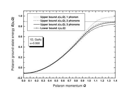
Figure 1: Dispersion of 1D polaron in GaAs

General formulae and some numerical results for a three-phonon exchange as well as a lower bound can be found in Ref. kalina . Here they are presented in Fig. 1 for a very small value of the coupling constant $\alpha=0.068$ corresponding to a real material (GaAs).

IV Fitting formula

To give an idea of typical values of the Fröhlich coupling constant for other materials, we present here some experimental data from Ref. karth : $\alpha=0.022$ for InSb, $\alpha=0.123$ for AlAs, $\alpha=0.65$ for ZnS, $\alpha=1.84$ for AgCl. It is well known that intermediate values $\alpha\sim 1$ and even larger can be tackled within conventional Raleigh-Schrödinger perturbations. This becomes possible because the coefficients $e_{n}$ in the expansion $E(\alpha,0)=\sum_{n}e_{n}\alpha^{n}$ of the polaron ground-state energy decrease very fast with $n$ so that the expansion is performed, roughly speaking, in powers of $\alpha/10$ or so. One can notice this tendency (although it is not proved rigorously) looking at Eq. (37). The famous Feynman approximation feynman clearly demonstrates this property as it follows from our calculations smond2 of first twelve (sic!) coefficients of the weak-coupling expansion for the 3D-polaron. Besides, the radius of convergence $R_{\alpha}$ of the RSPT for the bulk polaron ground-state energy was estimated in a number of papers: Larsen larsen2 found $R_{\alpha}\sim 6.2\div 6.5$, Klochikhin klochikhin argued that $R_{\alpha}\sim 3.4$, our estimate smond2 gave $R_{\alpha}\sim 6.9$.

Anyway, this explains why the weak coupling expansion can be applied for intermediate values $\alpha\sim 1$ or even larger. On the other hand, our lower bound gives very poor results for the intermediate coupling. In addition, the two-phonon approximation works not so well at these values of the coupling constant $\alpha$. The reason is that the edge point $E(\alpha,0)+1$ is then calculated within the one-phonon approximation, which is certainly not enough to reach appropriate accuracy.

Taking as an example 1D-polaron, $E_{1ph}(\alpha,0)$ is defined as $z$ of Eq. (18) at $Q=0$:

$$E_{1ph}(\alpha,0)\sqrt{1-E_{1ph}(\alpha,0)}=-\alpha{\pi\over 2}.$$ (21)

Expanding $E_{1ph}(\alpha,0)$ in powers of $\pi\alpha/2$ we obtain $E_{1ph}(\alpha,0)=-(\alpha\pi/2)+(1/2)(\alpha\pi/2)^{2}+{\cal{O}}(\alpha)^{3}$. Here the second order coefficient is positive and equals one-half, while in the correct result peet2

$$E_{1ph}(\alpha,0)=-\left({\alpha\pi\over 2}\right)-\left({3\sqrt{2}\over 4}-1\right)\left({\alpha\pi\over 2}\right)^{2}+{\cal{O}}(\alpha)^{3}$$

it is small (-0.06) and negative. From the point of view of diagrammatic technique for polaronssmond it means that only the disconnected Feynman diagram is taken into account in the one-phonon approximation. In this approximation the contribution of two connected diagrams is skipped which otherwise would compensate rather a large positive coefficient to give a small negative residue -0.06. An analogous fine tuning happens for flat ($D=2$) and bulk ($D=3$) polarons as well.

This explains why one needs to include three-phonon amplitudes to describe not only weak couplings but also intermediate values $\alpha\sim 1$. However, as was mentioned earlier, three-phonon calculations can be performed only in $D=1$, and the numerical job becomes enormous in other spatial dimensions. So we propose now a simple formula to fit the exact dispersion curves. We demonstrate its validity for $D=1$ by the comparison with the three-phonon approximation. In other sections of the current paper the fitting formula will be used instead of the absent numerical three-phonon calculations.

Let us stress that we are not going to proceed to the strong-coupling limit. We are still dealing with the weak couplings and our goal is to restore what is lost in approximations with partial summation of the perturbation series, that is to regain a possibility to use the weak-coupling results for the intermediate values of $\alpha$.

We start with the first term of the Brillouin-Wigner perturbation series (18) which reproduces the general behavior of the dispersion curve. As we already know, its main disadvantage is the lack of accuracy, especially in calculating the value of the continuum edge. Thus, we propose to remedy this weak point introducing correction terms ”by hand”.

First of all, we replace the first order expression for the ground-state energy (which equals $-\alpha\pi/2$ in this case) by its exact value $E(\alpha,0)$. Then we also replace the approximate edge point which is unity by its exact value $1+E(\alpha,0)$ in the propagator of the r.h.s. of Eq. (18). Note that actually this step is not an approximation: the energy can be arbitrarily shifted in the denominators of the Brillouin-Wigner expansion, as was mentioned in Ref. lindemann . This allows us to keep the correct gap between the zone’s bottom and the edge point. Finally, we scale the total momentum $Q$ by the factor $b_{1}$ to obtain the correct effective mass behavior of the type $E(\alpha,Q)\approx E(\alpha,0)+Q^{2}/m(\alpha)$ at small $Q$. This way we arrive at our fitting formula:

$$f = (b_{1}Q)^{2}+{E(\alpha,0)\over\sqrt{1+E(\alpha,0)-f}},$$

$$b_{1}^{2} = {1\over m(\alpha)}\left(1-{E(\alpha,0)\over 2}\right).$$

Later we apply a similar procedure to the cases $D=2,3$.

At small $Q$ the correct parabolic behaviour is guaranteed by the very construction of Eq. (LABEL:interp1d). When $Q$ is large it leads to the asymptotic behaviour

$$f\approx 1+E(\alpha,0)-{(E(\alpha,0))^{2}\over(b_{1}Q)^{4}}+\dots$$ (23)

Thus, the dispersion curve approaches the correct continuum edge rather fast.

The exact expressions for the polaron ground-state energy $E(\alpha,0)$ and its effective mass $m(\alpha)$ are unknown but they can be calculated numerically with the help of the perturbation series. The first two terms of the latter were found in Ref. peet2 and a few next terms were calculated by Khomyakovkhomyak :

$$E(\alpha,0) = -{\alpha\pi\over 2}-0.060660\left({\alpha\pi\over 2}\right)^{2}-0.00844437\left({\alpha\pi\over 2}\right)^{3}$$

$$-0.00151488\left({\alpha\pi\over 2}\right)^{4},$$

$$m(\alpha) = 1+0.5\left({\alpha\pi\over 2}\right)+0.191942\left({\alpha\pi\over 2}\right)^{2}$$ (24)

$$+0.0691096\left({\alpha\pi\over 2}\right)^{3}.$$

The results for $\alpha=0.5$ are presented in Fig. 2, where numerically exact ground-state energy $E(\alpha,0)$ and the edge-point $1+E(\alpha,0)$ are shown by solid thin straight lines.

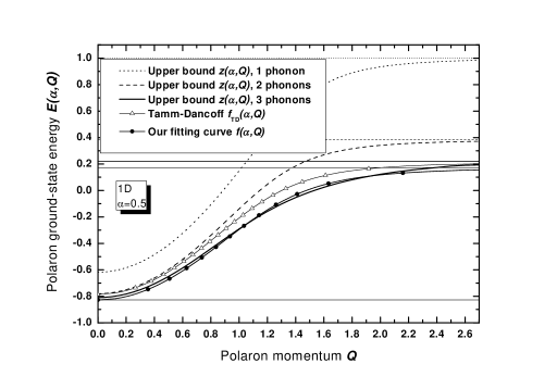
Figure 2: Dispersion of 1D polaron for $\alpha=0.5$

Our fitting formula is close to the so-called improved Brillouin-Wigner perturbation theory of Ref. lindemann which appears to be equivalent to the one-phonon Tamm-Dancoff approximation whit . Previously, this approximation was used for polarons in $D=2,3$ (the discussion and references will be given later). With these ideas being applied to the polaron in 1D, we obtain the following expression:

$$f_{TD} = Q^{2}-{\alpha\pi/2\over\sqrt{1-\alpha\pi/2-f_{TD}}}.$$ (25)

In comparison with our Eq. (LABEL:interp1d) only the first order in $\alpha$ is taken into account for the polaron ground state energy at rest and the effective mass (which gives $b_{1}=1$). The curve $f_{TD}$ is also plotted in Fig. 2.

Comparing with the three-phonon calculation one can notice that our fitting curve provides us with an excellent result which is also better than the Tamm-Dancoff approximation. This is not surprising because we used in our construction the RSPT expansions to rather high orders which work quite well for the intermediate values of $\alpha$. Thus, analogous fitting formulas will help us in the next sections where it is not possible technically to perform calculations within the three-phonon approximation to proceed to the region of intermediate couplings.

V The 2D case

With the one-phonon exchange taken into account (the same Eqs. (4) and (7) taken for $D=2$) we arrive at the equation for the upper bound:

$$z=Q^{2}-{\alpha\over\sqrt{Q^{2}+1-z}}\ K\left({Q^{2}\over Q^{2}+1-z}\right).$$ (26)

If we put $z=Q^{2}$ in the r.h.s. of Eq. (26), we get the expression for the first order of the RSPT given by Eq. (2b).

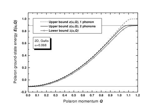
Figure 3: Dispersion of 2D polaron in GaAs

The results obtained with this formula and with the two-phonon exchange as well as the lower bound are presented in Fig. 3 for $\alpha=0.068$. Numerical calculations for the three-phonon exchange are very complicated and, therefore, will not be performed in this case. However, for such a small value of $\alpha$ the gap between the upper and lower bounds is very narrow.

To tackle intermediate values of $\alpha$, we apply the same idea to construct a fitting formula which reads in 2D as follows:

$$f = (b_{2}Q)^{2}+{2\over\pi}{E(\alpha,0)\over\sqrt{(b_{2}Q)^{2}+1+E(\alpha,0)-f}}$$

$$\times K\left({(b_{2}Q)^{2}\over(b_{2}Q)^{2}+1+E(\alpha,0)-f}\right),$$

$$b_{2}^{2} = {1\over m(\alpha)}\left(1-{E(\alpha,0)\over 4-E(\alpha,0)}\right).$$

Here again the correct parabolic behaviour at small $Q$ is reproduced by the very construction of the fitting formula. The asymptotic behavior of the complete elliptic integral $K(m)\sim-(1/2)\ln(1-m/16)$ when $m\to 1$ leads to the following asymptotics of the dispersion curve at large $Q$:

$$f\approx 1+E(\alpha,0)-16(b_{2}Q)^{2}\exp[-{\pi(b_{2}Q)^{3}\over|E(\alpha,0)|}]+\dots$$ (28)

Thus, the dispersion curve approaches the continuum edge extremely fast.

The expressions for the $2D$-polaron ground-state energy and effective mass can be taken from Ref. devr ; selugin :

$$E(\alpha,0) = -{\pi\over 2}\alpha-0.063974\alpha^{2},$$

$$m(\alpha) = 1+{\pi\over 8}\alpha+0.127235\alpha^{2}.$$ (29)

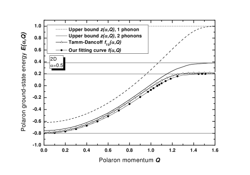
Figure 4: Dispersion of 2D polaron for $\alpha=0.5$

The Tamm-Dancoff approximation for the 2D polaron was calculated by the Antwerp groupwarmenbol . Again, the formula is very similar to our Eq. (LABEL:eq2dfit), where $b_{2}$ is replaced by unity and $E(\alpha,0)$ is put equal to $-\alpha\pi/2$:

$$f_{TD} = Q^{2}-{\alpha\over\sqrt{Q^{2}+1-\alpha\pi/2-f_{TD}}}$$ (30)

$$\times K\left({Q^{2}\over Q^{2}+1-\alpha\pi/2-f_{TD}}\right).$$

The numerical results are shown in Fig. 4.

VI The 3D case

With Eqs. (4) and (7) the result of the one-phonon approximation for the bulk polaron ($D=3$) reads as follows:

$$z=Q^{2}-{\alpha\over Q}\arcsin{Q\over\sqrt{Q^{2}+1-z}}.$$ (31)

This equation appeared at first in Ref.zienau . Putting $z=Q^{2}$ in the r.h.s. of Eq. (31) we get the expression for the first order of the RSPT given by Eq. (2c).

Being expanded in powers of the coupling constant this reproduces at $Q=0$ the exact results to the first order in $\alpha$:

$$z(\alpha,0)=-\alpha+{\cal O}(\alpha^{2}).$$ (32)

For the edge point we have again $z_{c}=1$. Inserting this value into Eq. (31) we obtain the equation for the value $Q_{c}$ at which the edge point is reached:

$$Q_{c}(Q_{c}^{2}-1)=\alpha{\pi\over 2}.$$ (33)

In this approximation the curve $z(\alpha,Q)$ approaches the edge point $z(\alpha,Q_{c})=1$ as an inverse parabola:

$$z(\alpha,Q)\approx 1-{Q_{c}^{2}(3Q_{c}^{2}-1)\over\alpha^{2}}(Q_{c}-Q)^{2}$$ (34)

at $Q\approx Q_{c},Q<Q_{c}$.

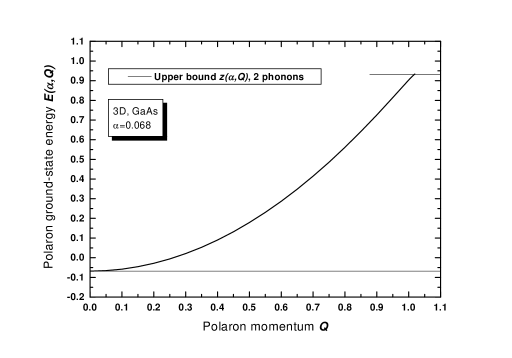
Figure 5: Dispersion of 3D polaron in GaAs

The curve for the upper bound which we calculated within the two-phonon approximation for GaAs is shown in Fig. 5. In the whole range of momentum $Q$ it is almost undistinguishable from the lower and upper bounds within the one-phonon approximation. Thus, it can be considered as a (numerically) exact result. All three curves are presented near the edge point in Fig. 6. The curvature of the dispersion near the edge point is very large at small $\alpha$, as it follows from Eq. (34), and the inverse parabola described by this equation can hardly be seen in these plots.

Again the gap between the edge point and the zone’s bottom is larger than the phonon energy (unity) in the one-phonon approximation. There is no physical reasons for that, and this disadvantage was removed in Ref. whit . However, the authors obtained wrong weak-coupling expansions for the polaron energy and effective mass at small momenta. A modification of Eq. (31) was given by Klochikhinklochikhin who studied the 3D polaron dispersion in the scope of the perturbation theory and took into account two-phonon amplitudes. This way he arrived at the following equation:

$$f_{TD}=Q^{2}-{\alpha\over Q}\arcsin{Q\over\sqrt{Q^{2}+1-\alpha-f_{TD}}},$$ (35)

which coincides with the Tamm-Dancoff approximation warm2 . This way he obtained the value $E_{c}\approx 1-\alpha$ for the continuum edge in the first order in $\alpha$ which is reached at $Q_{c}=1.16$. The correct energy shift was the advantage of these calculations in comparison with previously made in Ref. whit .

Figure 6: Dispersion of 3D polaron in GaAs near the edge point

For intermediate values of $\alpha$ (we present here examples with $\alpha=0.5,1$) the two-phonon exchange contribution does not provide us with impressive results. The three-phonon contribution requires a very large amount of computational work and, therefore, will not be given here. Besides, such values of $\alpha$ are outside the domain admissible for the lower bound, although the polaron is still in the weak-coupling regime. So we again construct our fitting formula which now takes the form:

$$f = (b_{3}Q)^{2}+{E(\alpha,0)\over b_{3}Q}\arcsin{b_{3}Q\over\sqrt{(b_{3}Q)^{2}+1+E(\alpha,0)-f}},$$

$$b_{3}^{2} = {1\over m(\alpha)}\left(1-{E(\alpha,0)\over 6-2E(\alpha,0)}\right).$$ (36)

Note that at $b_{3}=1$ and $E(\alpha,0)=-\alpha$ this equation reduces to Eq. (35).

The bulk polaron ground state energy and its effective mass are given by the known perturbation series (the second order in $\alpha$ was found in Ref. roseler and the third order was calculated in Ref. smond ; smond2 :

$$E(\alpha,0) = -\alpha-1.59196(\alpha/10)^{2}-0.80607(\alpha/10)^{3},$$

$$m(\alpha) = 1+\alpha/6+2.36276(\alpha/10)^{2}.$$ (37)

The maximal value $Q_{c}$ of the polaron momentum can be found from the fitting formula (36) if we put $f=1+E(\alpha,0)$. Then we arrive at the equation for $Q_{c}$:

$$Q_{c}=q_{c}/b_{3},$$

$$q_{c}\left(q_{c}^{2}-1-E(\alpha,0)\right)=-{\pi\over 2}E(\alpha,0).$$ (38)

The fitting dispersion curve $f(\alpha,Q)$ approaches the edge point also as an inverse parabola at $Q\approx Q_{c},Q<Q_{c}$:

$$f(\alpha,Q) \approx 1+E(\alpha,0)$$ (39)

$$- {q_{c}^{2}(3q_{c}^{2}-1-E(\alpha,0))^{2}\over E(\alpha,0)^{2}}(q_{c}-q)^{2},$$

where $q=b_{3}Q$.

This way we found $Q_{c}=1.02$ for $\alpha=0.068$, $Q_{c}=1.11$ for $\alpha=0.5$, and $Q_{c}=1.20$ for $\alpha=1$. The fitting curves obtained are shown in Figs. 7 and 8 together with one- and two-phonon calculations. Being applied at $\alpha=0.068$ this procedure leads practically to the same results as direct calculations.

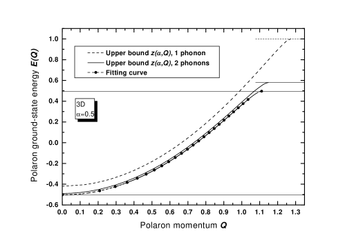
Figure 7: Dispersion of 3D polaron for $\alpha=0.5$

The results of the Monte-Carlo calculationsprokofiev ; prokofiev2 are shown also in Fig. 8. The relation $k=Q\sqrt{2}$ is used between our momentum $Q$ and their momentum $k$ (free electron energy reads as follows: $E=Q^{2}=k^{2}/2$). We see excellent agreement between our results almost in the whole range of momentum except for the vicinity of the edge point. The Monte-Carlo calculations give the value $Q_{c}^{MC}\approx 1.285$ while our fitting formula gives $Q_{c}^{fit}=1.20$. This discrepancy of 8% is responsible for the deviation of these curves. The authors of Refs. prokofiev ; prokofiev2 reported that their calculations were ”numerically exact” and the error bars were smaller than the size of points at the plot. Previously, kalina we criticized these statements, in particular, because the results obtained give the wrong coefficient even in the second order in $\alpha$ for the polaron ground state energy weak-coupling expansion. As we could see above, the correct second order calculations are crucial for the adequate description of the dispersion near the edge point.

The polaron dispersion $f(\alpha,Q)$ was also calculated by Larsen larsen who combined for his variational ansatz the one-phonon Tamm-Dancoff approximation and the Lee-Low-Pines transformation lee :

$${f_{L}+\alpha-Q^{2}\over f_{L}+\alpha+Q^{2}}={2\alpha\over\pi}F(\alpha,Q),$$

$$F(\alpha,Q)=\int_{0}^{\infty}dk{k^{2}\over(1+k^{2})^{2}}\cdot$$

$$\cdot\int_{-1}^{1}d\xi{\xi^{2}\over f_{L}+\alpha-1-Q^{2}-k^{2}+2Qk\xi}.$$ (40)

Both the Tamm-Dancoff approximation (35) and the calculations with Eq. (40) are shown in Fig. 8. Our curve is very close to Larsen’s one although they lead to different values of the edge point momentum ($Q_{c}^{Lar}\approx 1.25$). On the other hand, Larsen’s curve tends to a higher (and wrong) value of the polaron energy at the edge point and this is the main source of the discrepancy in calculating $Q_{c}$. However, if we recall that the correct edge point value $1+E(\alpha,0)$ is the rigorous upper bound for the dispersion (see Eq. (1)), we have to find the momentum at which Larsen’s curve reaches it. This way we found practically the same $Q_{c}\approx 1.20$ as given by our fitting formula. Thus, we arrive at the same results for $Q_{c}$ although Larsen’s Eq. (40) and our Eq. (36) do not look similar and were obtained in different ways. This gives hope that the value of $Q_{c}=1.20$ found for $\alpha=1$ fits the exact one quite well.

Figure 8: Dispersion of 3D polaron for $\alpha=1$

VII Conclusions

We have presented here the upper and lower bounds for the polaron dispersion in $D=1,2,3$. At small values of the electron-phonon coupling constant $\alpha$ the gap between our estimates is so narrow that we report in reality numerically exact results.

For intermediate values of $\alpha\approx 1$ we proposed the fitting formula which is simple to use in numerical calculations. Its validity is proved by comparing with the direct three-phonon calculations for the $1D$-polaron. For $D=2,3$ the comparison with the previously obtained results is also made, which allows us to conclude that the proposed formula fits the exact dispersion quite well in all space dimensions.

References

- (1) H. Fröhlich, H. Pelzer, and S. Zienau, Phil. Mag. 41, 221 (1950).
- (2) G. Whitfield, and R. D. Puff, Phys. Rev. 139, A338 (1965).
- (3) J. Appel, Polarons, in: Solid State Physics (Advances in Research and Applications), 21, ed. by F. Seitz, D. Turnbull and H. Ehrehreich (Academic Press, New York, 1968), p. 193.
- (4) B. Gerlach, and H. Löwen, Rev. Mod. Phys. 63, 63 (1991).
- (5) H. Spohn, Ann. Phys. 175, 278 (1987).
- (6) T. D. Lee, F. E. Low, and D. Pines, Phys. Rev. 90, 297 (1953); 91, 227 (1953).
- (7) D. M. Larsen, Phys. Rev. 144, 697 (1966). D. M. Larsen, in: Polarons in Ionic Crystals and Polar Semiconductors, ed. J. T. Devreese, (North-Holland, Amsterdam, 1972), p. 237.
- (8) P. Warmenbol, F. M. Peeters, and J. T. Devreese, Phys. Rev. B 33, 5590 (1986).
- (9) F. M. Peeters, P. Warmenbol, and J. T. Devreese, Europhys. Lett. 3, 1219 (1987).
- (10) E. Lieb, and K. Yamazaki, Phys. Rev. 111, A 728 (1958). See also E. Lieb, and L. Thomas, Comm. Math. Phys. 183, 511 (1997); Erratum: Comm. Math. Phys. 188, 499 (1997).
- (11) B. Gerlach, and F. Kalina Phys. Rev. B 60, 10886 (1999).
- (12) F. M. Peeters, Wu Xiaoguang, and J. T. Devreese, Phys. Rev. B 33, 3926 (1986).
- (13) F. M. Peeters, and M. A. Smondyrev, Phys. Rev. B 43, 4920 (1991).
- (14) B. Gerlach, and H. Löwen, Phys. Rev. B 35, 4291 (1987).
- (15) B. Gerlach, F. Kalina, and M. A. Smondyrev, phys. stat. sol. (b) 237, 204 (2003).
- (16) H. Spohn, J. Phys. A 21, 1199 (1988).
- (17) E. Kartheuser, in: Polarons in Ionic Crystals and Polar Semiconductors, ed. J. T. Devreese, (North-Holland, Amsterdam, 1972), p. 717.
- (18) R. P. Feyman. Phys. Rev. 84, 108 (1951).
- (19) O. V. Selyugin, and M. A. Smondyrev, phys. stat. sol. (b) 155, 155 (1989).
- (20) D. Larsen, Phys. Rev. 187, 1147 (1969).
- (21) A. A. Klochikhin, Fiz. Tverd. Tela 21, 3077 (1979) [Sov. Phys. - Solid State 21, 1770 (1980)].
- (22) M. A. Smondyrev, Teor. Mat. Fiz. 68, 29 (1986) [Theor. Math. Phys. 68, 653 (1987)].
- (23) G. Lindemann, R. Lassnig, W. Seidenbusch, and E. Gornik, Phys. Rev. B 28, 4693 (1983).
- (24) P. A. Khomyakov, Phys. Rev. B 63, 153405-1 (2001).
- (25) Wu Xiaoguang, F. M. Peeters, and J. T. Devreese, Phys. Rev. B 31, 3420 (1985).
- (26) O. V. Seljugin, and M. A. Smondyrev, Physica 142A, 555 (1987).
- (27) J. Röseler, phys. stat. sol. 25, 311 (1968).
- (28) N. V. Prokof’ev, and B. V. Svistunov, Phys. Rev. Lett. 81, 2514 (1998).
- (29) A. S. Mischenko, N. V. Prokof’ev, A. Sakamoto, and B. V. Svistunov, Phys. Rev. B 62, 6317 (2000).