Hierarchy of inequalities for quantitative duality

Abstract

We derive different relations quantifying duality in a generic two-way interferometer. These relations set different upper bounds to the visibility $\mathcal{V}$ of the fringes measured at the output port of the interferometer. A hierarchy of inequalities is presented which exhibits the influence of the availability to the experimenter of different sources of which-way information contributing to the total distinguishability $\mathcal{D}$ of the ways. For mixed states and unbalanced interferometers an inequality is derived, $\mathcal{V}^{2}+\Xi^{2}\leq 1$, which can be more stringent than the one associated with the distinguishability ($\mathcal{V}^{2}+\mathcal{D}^{2}\leq 1$).

I INTRODUCTION

The principle of complementarity is one of the mayor cornerstones of Quantum Mechanics Feynman65 . The implications of this principle continue to nurture debates in quantum theory Einstein . A new inequality has been introduced todos ; Jaeger95 ; Englert96 that quantifies the notion of duality in the context of two-way interferometers. This inequality has attracted great interest both theoretically Bjork98 ; Englert2000 and experimentally DurrNature98 ; Englert99 ; Durr2000 . The inequality establishes an upper bound to the fringe visibility $\mathcal{V}$ displayed by a two-level system (the “quanton”) at the output port of a two-way interferometer. This bound is given by the distinguishability $\mathcal{D}$, i.e., the maximum amount of which-way information (WWI) that can be potentially available to the experimenter Englert96 ; namely,

$$\mathcal{V}^{2}\leq 1-\mathcal{D}^{2}.$$ (1)

However, two different sources of WWI contributes to $\mathcal{D}$. One is the a-priori WWI given by the predictability $\mathcal{P}$ of the ways, i.e., the a priori which-way knowledge that the experimenter has about the ways stemming from the preparation of the beam splitter (BS) and the initial state of the quanton. $\mathcal{P}$ is a measure of WWI on its own. In fact, it satisfies the inequality todos ; Englert96

$$\mathcal{V}^{2}\leq 1-\mathcal{P}^{2}.$$ (2)

In addition, the experimenter may place a quantum memory system to interact with the quanton in order to acquire extra WWI, i.e., to serve as a which-way marker (WWM). Thus, the second source of WWI stems from the WWM’s ability to correlate its final states with the two ways, leading to the storage of some WWI. A measure of the quantum “quality” $\mathcal{Q}$ of the WWM has been introduced in Jesus04 . We will show that this quantity also obeys an inequality of the same type, i.e.,

$$\mathcal{V}^{2}\leq 1-\mathcal{Q}^{2}.$$ (3)

Moreover, the final visibility is limited by the availability of both kinds of WWI by the inequality

$$\mathcal{V}^{2}\leq\left(1-\mathcal{P}^{2}\right)\left(1-\mathcal{Q}^{2}\right).$$ (4)

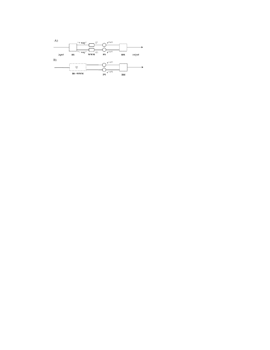
Figure 1: Schematic two-way interferometer setup composed of a beam splitter (BS), a quantum which-way marker (WWM), a phase shifter (PS), and a beam merger (BM). (a) The WWM is characterized by unitary $U_{\pm}$ evolution. (b) Quantized BS: in this general case the same physical interaction is used for both splitting the beam and marking the way.

Equation (4) has been derived in Jesus04 for the special case of unitary WWM evolution [Fig.1(a)]. Here we will prove it for a generic two-way interferometer, i.e., the general case where WWM evolution can be non unitary, so quantum optical Ramsey interferometers newHaroche2001 can also be analyzed [Fig.1(b)]. Then, we show that for two-level WWM systems Eq. (4) can be more stringent than Eq. (1).

This scheme sets the organization of the paper. First we describe in Sec. II the formalism for generic two-way interferometers with non-unitary WWM. Section III is devoted to the derivation of Eqs. (3) and (4). In Sec. IV Eq. (4) is interpreted as an inequality quantifying duality. Here we also prove the stringency statement. In Sec. V the results are illustrated with the help of a simple example: the symmetric quantum-detecton system (a particular quantum logic gate). Finally we end up with conclusion and a summary of the results.

II NONUNITARY WWM

Let us consider the generic two-way interferometer plotted in Fig.1(b). Following the notation of Jesus04 the quanton is prepared initially in the state

$$\rho_{Q}^{(0)}=\frac{1}{2}\left(1+\bm{s}_{Q}^{(0)}\cdot\bm{\sigma}\right),$$ (5)

where $\bm{\sigma}=(\sigma_{x},\sigma_{y},\sigma_{z})$ are the usual Pauli spin operators, and $\bm{s}_{Q}^{(0)}=(0,0,s)$ is the polarization vector of the state, characterized by the inversion $s\in(-1,1)$. We now consider the most general case and include BS and WWM action into the same global action characterized by the operator $U$. The combined quanton-WWM system is initially prepared in the state $\rho^{(0)}=\rho_{Q}^{(0)}\otimes\rho_{D}^{(0)}$, where $\rho_{D}^{(0)}$ is an arbitrary initial state of the WWM. After interaction between the quanton and WWM, the evolution of the entire system is given by the unitary map $\rho\rightarrow U^{{\dagger}}\,\rho U$. We follow Englert’s notation Englert96b and write the general evolution operator in the quanton $\sigma_{z}$ base as

$$U=\frac{1}{\sqrt{2}}\left(\begin{array}[]{cc}V_{++}&V_{+-}\\ -V_{-+}&V_{--}\end{array}\right),$$ (6)

with the matrix elements acting exclusively on the WWM. These four operators are not necessarily unitary, though they are restricted by the unitarity of $U$. Note that the particular case $V_{++}=V_{-+}=U_{+}$, $V_{+-}=V_{--}=U_{-}$, with $U_{\pm}U_{\pm}^{\dagger}=U_{\pm}^{\dagger}U_{\pm}=I$ brings us back to the unitary case of Fig.1(a) studied in Jesus04 . Thus, the results of this paper cover both situations schematized in Figs. 1a-b.

Now is the turn of the phase shifter (PS), that effects the transition

$$\rho_{Q}\rightarrow\exp\left(-i\frac{\phi}{2}\sigma_{z}\right)\rho_{Q}\;\exp\left(i\frac{\phi}{2}\sigma_{z}\right),$$ (7)

and subsequently the beam merger (BM)

$$\rho_{Q}\rightarrow\exp\left(-i\frac{\pi}{4}\sigma_{y}\right)\rho_{Q}\;\exp\left(i\frac{\pi}{4}\sigma_{y}\right).$$ (8)

Combining transformations (6), (7) and (8), the general final state comentario inversion at the output port of the interferometer given in Fig.1(b) is

$$\rho^{(f)}=\frac{1+s}{2}\;\rho^{(f)}_{\uparrow}+\frac{1-s}{2}\;\rho^{(f)}_{\downarrow},$$ (9)

where

$$\rho^{(f)}_{\uparrow} = \mbox{$\frac{(1+\sigma_{x})}{4}$}\;V_{++}^{{\dagger}}\rho_{D}^{(0)}V_{++}+\mbox{$\frac{(1-\sigma_{x})}{4}$}\;V_{+-}^{{\dagger}}\rho_{D}^{(0)}V_{+-}$$ (10)

$$+ \mbox{$\frac{(-\sigma_{z}+i\sigma_{y})}{4}$}\,V_{++}^{{\dagger}}\rho_{D}^{(0)}V_{+-}\;e^{-i\phi}$$

$$- \mbox{$\frac{(\sigma_{z}+i\sigma_{y})}{4}$}\,V_{+-}^{{\dagger}}\rho_{D}^{(0)}V_{++}\;e^{i\phi}\,,$$

and $\rho^{(f)}_{\downarrow}$ can be obtained from the above equation through the replacements

$$V_{++}\rightarrow-V_{-+};\>\;V_{+-}\rightarrow V_{--}\;.$$ (11)

After tracing over the WWM’s degrees of freedom, the final state of the quanton can be expressed in terms of a Bloch vector $\bm{\sigma}^{(f)}$ with components

$$S_{Qx}^{(f)} = w_{+}-w_{-}\,,$$

$$S_{Qz}^{(f)} = -\frac{1+s}{2}\;\Re e\left[\mathcal{C}_{\uparrow}e^{-i\phi}\right]-\frac{1-s}{2}\;\Re e\left[\mathcal{C}_{\downarrow}e^{-i\phi}\right],$$

$$S_{Qz}^{(f)}+iS_{Qy}^{(f)} = -\;e^{-i\phi}\mathcal{C},$$ (12)

where

$$w_{\pm}=\mbox{tr}\left\{\frac{1\pm\sigma_{x}}{2}\rho^{(f)}\right\},$$ (13)

$w_{+}+w_{-}=1$, are the probabilities for taking the two alternative ways at the central stage of the interferometer, and

$$\mathcal{C}=\frac{1+s}{2}\;\mathcal{C}_{\uparrow}+\frac{1-s}{2}\;\mathcal{C}_{\downarrow},$$ (14)

with

$$\mathcal{C}_{\uparrow} \equiv \mbox{tr}_{D}\,\left\{V_{++}^{{\dagger}}\rho_{D}^{(0)}V_{+-}\right\}=\left<V_{+-}V_{++}^{{\dagger}}\right>_{0},$$

$$\mathcal{C}_{\downarrow} \equiv -\mbox{tr}_{D}\,\left\{V_{-+}^{{\dagger}}\rho_{D}^{(0)}V_{--}\right\}=-\left<V_{--}V_{-+}^{{\dagger}}\right>_{0}.$$ (15)

Inserting Eq. (9) into Eq. (13) the transition probabilities are calculated to be

$$w_{+} = \frac{1+s}{4}\;\left<V_{++}V_{++}^{{\dagger}}\right>_{0}+\frac{1-s}{4}\;\left<V_{-+}V_{-+}^{{\dagger}}\right>_{0},$$

$$w_{-} = \frac{1+s}{4}\;\left<V_{+-}V_{+-}^{{\dagger}}\right>_{0}+\frac{1-s}{4}\;\left<V_{--}V_{--}^{{\dagger}}\right>_{0}.$$ (16)

The mean value of their difference is the predictability of the ways, i.e.,

$$\mathcal{P}=|w_{+}-w_{-}|.$$ (17)

$\mathcal{P}$ is a-priori WWI. The x component of the Bloch vector given in (12) represents a priori WWI. The other components give information about complementary wavelike aspects of the quanton. In order to see this, let us focus on the output port of the interferometer. The probability of measuring the upper or lower state of the quanton, after many repetitions of the experiments, displays an interference pattern versus variation of the phase in the PS. The visibility of the fringes can be rapidly calculated with the help of (12) to yield

$$\mathcal{V}=\mid\mathcal{C}\mid\leq 1.$$ (18)

$\mathcal{C}$ is therefore a contrast factor. Inserting Eqs. (18) and (17) into Eq. (12), it is easy to check that the duality relation given in Eq. (2) is also valid for non-unitary WWM.

More stringent inequalities than (2) can be derived for the system. Englert Englert96b derives the inequality given in Eq. (1) for the distinguishability

$$\mathcal{D}=\text{tr}_{D}\{|w_{+}\rho_{D}^{(+)}-w_{-}\;\rho_{D}^{(-)}|\},$$ (19)

where

$$w_{+}\rho_{D}^{(+)} = \text{tr}_{Q}\left\{\frac{1+\sigma_{x}}{2}\;\rho^{(f)}\right\}$$

$$= \frac{1+s}{4}\;V_{++}^{{\dagger}}\rho_{D}^{o}V_{++}+\frac{1-s}{4}\;V_{-+}^{{\dagger}}\rho_{D}^{o}V_{-+},$$

$$w_{-}\rho_{D}^{(-)} = \text{tr}_{Q}\left\{\frac{1-\sigma_{x}}{2}\;\rho^{(f)}\right\}$$ (20)

$$= \frac{1+s}{4}\;V_{+-}^{{\dagger}}\rho_{D}^{o}V_{+-}+\frac{1-s}{4}\;V_{--}^{{\dagger}}\rho_{D}^{o}V_{--}.$$

$\rho_{D}^{(\pm)}$ are the final states of the WWM associated with a measure of the $\sigma_{z}=\pm 1$ way comentario BM . These states are normalized, so $\rho_{D}^{(f)}=\text{tr}_{Q}\;\rho^{(f)}=w_{+}\rho_{D}^{(+)}+w_{-}\rho_{D}^{(-)}$ is the final state of the WWM provided no measure of the ways is taken.

Two kinds of WWI are represented in $\mathcal{D}$. One is the predictability of the ways, given in (17). The other one is given by the quantum “quality” of the WWM, i.e., its ability to establish quantum correlations with the quanton, leading to the storage of some WWI into the final state of the WWM. In Jesus04 the quality measure

$$\mathcal{Q}=\frac{1}{2}\;\text{tr}_{D}\{\mid\rho_{D}^{(+)}-\rho_{D}^{(-)}|\}$$ (21)

has been introduced. $\mathcal{Q}$ is a distance between the conditional probabilities $\rho_{D}^{(+)}$ and $\rho_{D}^{(-)}$ in the trace-class norm. Note that for balanced interferometers ($\mathcal{P}=0$), $\mathcal{Q}$ coincides with $\mathcal{D}$. Otherwise their value may substantially differ. In both cases $\mathcal{Q}$ is a quantitative measure of the WWM’s intrinsic ability to distinguish between the quanton’s alternatives. For $\mathcal{Q}=0$ the marker cannot distinguish the ways at all. Conversely, full WWI can be stored in the marker when $\mathcal{Q}=1$. The states $\rho_{D}^{(\pm)}$ can be prepared if we modify the interferometer such that the actual way taken by the quanton is measured rather than the fringe pattern. Thus, the value of $\mathcal{Q}$ can be experimentally measured along the same lines described in Englert96 ; Englert99 for measuring $\mathcal{D}$.

III More inequalities

In Jesus04 we restricted the analysis for the particular case of unitary matrix elements in (6), so (21) is a distance between projectors. Here, we release this condition and prove the validity of Eq. (4) in the general case.

The validity of Eq. (1) for nonunitary WWM has been given by Englert in Englert96b . Following Englert, we separate first both contributions on the right side of Eqs. (20) so

$$\mathcal{Q}_{\uparrow}=\frac{1}{4}\;\text{tr}_{D}\left\{\left|\frac{V_{++}^{{\dagger}}\rho_{D}^{(0)}V_{++}}{w_{+}}-\frac{V_{+-}^{{\dagger}}\rho_{D}^{(0)}V_{+-}}{w_{-}}\right|\right\},$$ (22)

gives the value of the quality $\mathcal{Q}$ for the $s=1$ case. For the $s=-1$ case, $\mathcal{Q}_{\downarrow}$ can be obtained from (22) by taking the replacements (11). The triangle inequality $\text{tr}\left\{\mid X+Y\mid\right\}\leq\text{tr}\left\{\mid X\mid\right\}+\text{tr}\left\{\mid Y\mid\right\}$ applied to (21) yields

$$\mathcal{Q}\leq\frac{1+s}{2}\;\mathcal{Q}_{\uparrow}+\frac{1-s}{2}\;\mathcal{Q}_{\downarrow}.$$ (23)

According to this notation and using (18), the duality relation given in (4) can be written for the particular cases $s=1$ ($\uparrow$) and $s=-1$ ($\downarrow$) as

$$\mathcal{Q}_{\uparrow\downarrow}^{2}+\frac{|C_{\uparrow\downarrow}|^{2}}{1-\mathcal{P}^{2}}\leq 1.$$ (24)

Here, we prove the $s=1$ case. The $s=-1$ case will follow straightforwardly, once the replacements (11) are taken. In order to do this, let us define the traceless operator

$$\Gamma=\frac{1}{2}\;\{\rho_{D}^{(+)}-\rho_{D}^{(-)}\},$$ (25)

Its eigenvalues are of the form $\pm\lambda$, so we can write

$$\mathcal{Q}=2|\lambda|.$$ (26)

To calculate $\lambda$, we use the relation $\text{tr}_{D}\,\Gamma^{2}=2\lambda^{2}$, and

$$4\text{tr}_{D}\,\Gamma^{2} = \text{tr}_{D}\{\rho_{D}^{(+)2}\}+\text{tr}_{D}\{\rho_{D}^{(-)2}\}$$ (27)

$$- \text{tr}_{D}\{\rho_{D}^{(+)}\rho_{D}^{(-)}\}-\text{tr}_{D}\{\rho_{D}^{(+)}\rho_{D}^{(-)}\}.$$

We particularize for the WWM’s pure state preparation, where we can work out explicitly the above four contributions. In fact, each of the first two terms is unity, in both the unitary and nonunitary cases. Next, we calculate the cross terms in (27). From the definitions (20) and (15) we have

$$\text{tr}_{D}\{\rho_{D}^{(+)}\rho_{D}^{(-)}\}=\frac{\mid C_{\uparrow}\mid^{2}}{4w_{+}w_{-}}=\text{tr}_{D}\{\rho_{D}^{(-)}\rho_{D}^{(+)}\}.$$ (28)

Collecting terms, we obtain

$$2\,\text{tr}_{D}\,\Gamma^{2}=1-\frac{\mid C_{\uparrow}\mid^{2}}{1-\mathcal{P}^{2}},$$ (29)

where the relation $1-\mathcal{P}^{2}=4w_{+}w_{-}$ has been used. Finally, using (29), (26) and (11) we obtain the pure state result

$$\mathcal{Q}_{\uparrow\downarrow}^{2}+\frac{\mid C_{\uparrow\downarrow}\mid^{2}}{1-\mathcal{P}^{2}}=1.$$ (30)

Now consider the general case where we prepare the WWM in a mixed state. Its spectral decomposition allow us to write it as a combination of pure states for which (30) can be applied; namely,

$$\rho_{D}^{(0)}=\sum_{k=1}^{N}D_{k}\mid d_{k}\rangle\langle d_{k}\mid,$$ (31)

where $\sum_{k}D_{k}=1$ and $\langle d_{k}\mid d_{j}\rangle=\delta_{kj}$. Inserting (31) into (22), and applying the triangular inequality we obtain

$$\mathcal{Q}_{\uparrow}\leq\sum_{k}D_{k}\;\mathcal{Q}_{\uparrow k},$$ (32)

where

$$\mathcal{Q}_{\uparrow k} = \text{tr}_{D}\left\{\left|\frac{V_{++}^{{\dagger}}\mid d_{k}\rangle\langle d_{k}\mid V_{++}}{w_{+}}-\frac{V_{+-}^{{\dagger}}\mid d_{k}\rangle\langle d_{k}\mid V_{+-}}{w_{-}}\right|\right\},$$

is the quality for pure state preparation and, thus, obeys (30). Therefore, Eq. (32) can be written as

$$\mathcal{Q}_{\uparrow}\leq\sum_{k}D_{k}\;\sqrt{1-\frac{\mid C_{\uparrow k}\mid^{2}}{1-\mathcal{P}^{2}}}\;,$$ (34)

where $C_{\uparrow k}=\langle d_{k}\mid V_{+-}V_{++}^{{\dagger}}\mid d_{k}\rangle$. We can also calculate $C_{\uparrow}$ in terms of pure state contributions. In fact, inserting (31) into (15) one obtains $C_{\uparrow}=\sum_{k}D_{k}\;C_{\uparrow k}$. Combining the two last summations, one gets

$$\mathcal{Q}_{\uparrow}^{2}+\frac{\mid C_{\uparrow}\mid^{2}}{1-\mathcal{P}^{2}}\leq\sum_{kj}D_{k}D_{j}\;$$

$$\times\left[\sqrt{1-\frac{\mid C_{\uparrow k}\mid^{2}}{1-\mathcal{P}^{2}}}\;\sqrt{1-\frac{\mid C_{\uparrow j}\mid^{2}}{1-\mathcal{P}^{2}}}+\frac{\mid C_{\uparrow k}\mid\mid C_{\uparrow j}\mid}{1-\mathcal{P}^{2}}\right].$$ (35)

Let us have a closer look on the matrix term in square brackets $[\;]_{kj}$ in the above equation. Its diagonal terms satisfy $[\;]_{kk}=1$, as can be checked by inspection. In order to prove that the non-diagonal terms are smaller than unity, let us define the numbers $\theta_{k}^{2}=|C_{\uparrow k}|^{2}/(1-\mathcal{P}^{2})$. Equation (30) implies $0\leq\theta_{k}\leq 1$, which are in turn duality relations of the type of Eq. (2). In terms of $\theta_{k}$, we can write $[\;]_{kj}=\sqrt{1-\theta_{k}^{2}}\sqrt{1-\theta_{j}^{2}}+\theta_{k}\theta_{j},$ which does not exceed unity. The calculation of the upper bound of (35) is now straightforward, namely,

$$\mathcal{Q}_{\uparrow}^{2}+\frac{\mid C_{\uparrow}\mid^{2}}{1-\mathcal{P}^{2}}\leq\sum_{kj}D_{k}D_{j}=1,$$ (36)

which completes the proof of the $s=1$ case of Eq. (24). Eq. (4) follows now directly from Eqs. (23) and (14). Moreover, Eq. (3) follows from Eq. (4), since $1-\mathcal{P}^{2}\leq 1$.

IV THE $\mathcal{V}_{\Xi}$ UPPER BOUND

We define the symmetric quantity

$$\Xi=\sqrt{\mathcal{Q}^{2}+\mathcal{P}^{2}-\mathcal{Q}^{2}\mathcal{P}^{2}}.$$ (37)

In terms of $\Xi$, Eq. (4) can be written as

$$\mathcal{V}^{2}+\Xi^{2}\leq 1.$$ (38)

Notice the high degree of symmetry inherent in the structure of Eq. (37). First, $\Xi$ is bounded by $\mathcal{Q}$ and $\mathcal{P}$. Actually, as can be rapidly checked in Eq. (37), $\Xi$ satisfies $0\leq\Xi\leq 1$, $\Xi\geq\mathcal{Q}$, $\Xi\geq\mathcal{P}$, $\Xi\geq\mathcal{Q}\;\mathcal{P}$, so is equal or greater than any of its two sources of WWI. This can be understood since $\Xi$ yields one kind of WWI, $\mathcal{Q}$ (or $\mathcal{P}$), when the other kind, $\mathcal{P}$ (or $\mathcal{Q}$), vanishes. For instance, for $\mathcal{P}=0$ we have $\mathcal{D}=\mathcal{Q}=\Xi$, i.e, for symmetric interferometers the inequalities given in Eqs. (38) and (3) reduces to the inequality given in Eq. (1).

Second, $\Xi$ reaches unity when any of its arguments $\mathcal{Q}$ (or $\mathcal{P})$ does, independently of the value of the other argument $\mathcal{P}$ (or $\mathcal{Q})$. In order to understand the importance of this property we note that Eq. (37) equals Eq. (19) in the case of pure state preparation ($|s|=1$, $\text{tr}_{D}\;\rho_{D}^{(0)2}=1$), i.e.,

$$\mathcal{D}^{2}=\Xi^{2}=\mathcal{P}^{2}+\mathcal{Q}^{2}(1-\mathcal{P}^{2}).$$ (39)

This can be shown by noting that in the pure-state case Eq. (30) turns into

$$\Xi^{2}+\mathcal{V}^{2}=1$$ (40)

and, on the other hand, Eq. (1) is satisfied as an equality Englert96b . Thus, for pure state preparation $\Xi$ coincides with $\mathcal{D}$, i.e., the total distinguishability of the ways. Equation (39) renders $\mathcal{P}$ and $\mathcal{Q}$ as two different contributions to the distinguishability. The condition $\mathcal{P}=1$ (or $\mathcal{Q}=1$) exhausts the amount of WWI needed to specify the actual path taken by the quanton, so $\mathcal{D}=1$ in each case, with independence of the value of the additional source of WWI.

Third, $\Xi$ treats on equal footing both sources of WWI since it is invariant under the permutation $\mathcal{P}\leftrightarrow\mathcal{Q}$. This fact, together with Eq. (40), tells us that for pure state preparation both sources of WWI stand on equal footing concerning wave-particle duality (WPD) degradation of fringe visibility.

Finally, Eq. (38) yields the following conditions

$$\mathcal{V}=1 \quad\Rightarrow\quad \Xi=\mathcal{P}=\mathcal{Q}=0,$$

$$\mathcal{P}=1 \quad\Rightarrow\quad \Xi=1,\mathcal{V}=0,$$

$$\mathcal{Q}=1 \quad\Rightarrow\quad \Xi=1,\mathcal{V}=0,$$

$$\Xi=1 \quad\Rightarrow\quad \mathcal{V}=0.$$ (41)

as demanded by duality. Thus, Eq. (38), like Eq. (1), is an inequality quantifying WPD. It devolves the extreme situations of Eqs. (41) showing that perfect fringe visibility and the acquisition of full path knowledge on any source of WWI are mutually exclusive. Intermediate situations of partial fringe visibility and partial WWI on each source are also contemplated in Eq. (38). Both equations (38) and (1) give quantitative statements about duality. Specifically, Eq. (38) allows one to trace the loss of coherence in asymmetric interferometers to the two reservoirs of WWI represented by $\mathcal{P}$ and $\mathcal{Q}$.

Now, the main result of the paper. We prove that there exists a wide class of systems where

$$\mathcal{V}^{2}\leq 1-\Xi^{2}\leq 1-\mathcal{D}^{2},$$ (42)

i.e., Eq. (4) (left-hand inequality above) can be more stringent than Eq. (1). In order to do so, we restrict ourselves to a generic two-level WWM [$N=2$ in Eq. (31)] and prove the inequality $\chi\equiv\mathcal{D}^{2}/\,\Xi^{2}\leq 1$, which is equivalent to the right hand side of (42). We use the relation $\mathcal{D}=\text{Max}\left\{\mathcal{P},\mathcal{R}\right\}$, with $\mathcal{R}^{2}=2\;\text{tr}_{D}\{\underline{\Delta}\}^{2}-\mathcal{P}^{2}$ and $\underline{\Delta}\equiv\omega_{+}\rho_{D}^{+}-\omega_{-}\rho_{D}^{-}$, which can be verified for $N=2$. For $\mathcal{P}\geq\mathcal{R}$, $\chi\leq 1$ follows trivially. For $\mathcal{P}<\mathcal{R}$ we compute explicitly both $\mathcal{D}$ and $\mathcal{Q}$ by diagonalizing Eqs. (19) and (21), respectively, along the same lines as used in the derivation of Eq. (30). After a rather lengthy calculation the result simplifies remarkably to the expression

$$\chi=1-\frac{4D_{1}D_{2}\mathcal{P}^{2}}{\Xi^{2}}\leq 1,$$ (43)

where we have taken for simplicity $|s|=1$ and $w_{\pm 12}=w_{\pm 21}^{*}=0$, $w_{\pm ij}$ being the matrix elements of the operators involved in Eq. (16).

Equation (42) defines two different upper bounds to the visibility, namely,

$$\mathcal{V}_{D} = \sqrt{1-\mathcal{D}^{2}},$$ (44)

$$\mathcal{V}_{\Xi} = \sqrt{1-\Xi^{2}}.$$ (45)

In terms of these bounds, Eqs. (1) and (38) can be rewritten as

$$\mathcal{V} \leq \mathcal{V}_{D},$$ (46)

$$\mathcal{V} \leq \mathcal{V}_{\Xi},$$ (47)

and Eq. (42) as

$$\mathcal{V}\leq\mathcal{V}_{\Xi}\leq\mathcal{V}_{D}.$$ (48)

Note that Eq. (46) does not saturate for mixed state preparation, so it is possible to find a stricter inequality. In fact, this is what has been accomplished in Eq. (48). Yet Eq. (47) does not saturate for mixed-state preparation comentario D=1 , so stricter inequalities could eventually still be found.

V AN EXAMPLE: THE SYMMETRIC DETECTON-QUANTON SYSTEM

In order to illustrate the formalism, we particularize it in this section to a concrete example: the symmetric quanton-detecton system (SQDS) Jesus04 . The SQDS is represented in Fig. 2. The system is basically a quantum logic gate in which each qubit (quanton and detecton) plays the role of which-way marker of the other. The conditional dynamics is achieved at the common phase shifter. The detecton phase shifter depends on the $\pm$ alternative ways of the quanton in the form

$$U_{PS}^{\pm}=\exp\left(\pm\frac{i}{2}\;\Phi\;\sigma_{Dz}\right),$$ (49)

where $\Phi$ is an entangling phase and $\sigma_{Dz}$ is the usual z component of the Pauli matrices for the detecton.

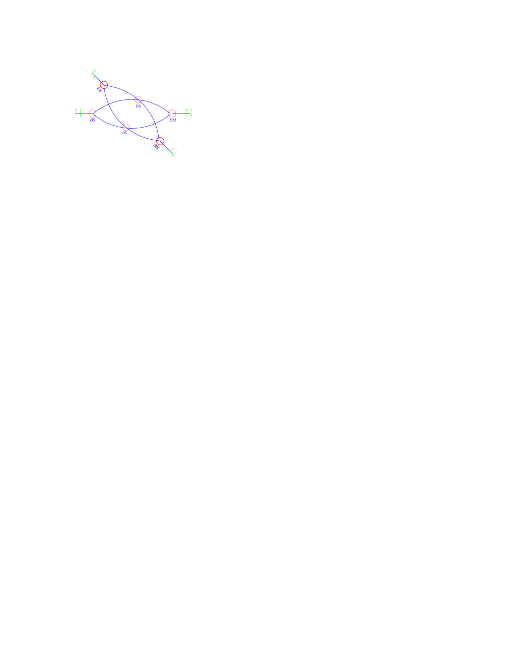
Figure 2: Schematic setup for the SQDS, showing the intrinsic symmetry between quanton and detecton.

On the other hand, the SQDS can be regarded as a pair of two-way interferometers coupled at their central stages by a dispersive interaction, trying to acquire WWI about each other. The detecton, like the quanton itself, is a two-way interferometer, likewise describable by a predictability $\mathcal{P}_{D}$ and a fringe visibility $\mathcal{V}_{D}^{o}$ satisfying

$$\mathcal{P}_{D}^{2}+\mathcal{V}_{D}^{o2}=|s_{D}^{(0)}|^{2}\leq 1,$$ (50)

where $\bm{s}_{D}^{(0)}$ is the Bloch vector describing the initial state of the detecton. We take the quanton prepared initially in a pure state so

$$\mathcal{P}_{Q}^{2}+\mathcal{V}_{Q}^{o2}=1.$$ (51)

The “quality” of the WWM is given in this model simply by

$$\mathcal{Q}_{D}=\mathcal{V}_{D}^{o}\;|\sin\Phi|.$$ (52)

$\mathcal{Q}_{D}$ characterizes “how good” the WWM is to establish quantum correlations leading to the acquisition of WWI about the quanton. Thus, the dependence of Eq. (52) on the entangling phase can be understood. The dependence on $\mathcal{V}_{D}^{o}$ is also important. As discussed in Jesus04 , as the detecton acquires WWI about the quanton it also degrades its own fringe visibility. This is due to the symmetric design of the SQDS, for which each qubit is the WWM of the other. According to duality in this reciprocal system, both qubits acquire WWI about each other and both degrade their visibility. Thus, the initial visibilities for quanton and detecton systems previous to their interaction act as limiting factors of their subsequent mutual transfer of WWI.

Now, we compute $\Xi$ for the quanton, i.e.,

$$\Xi_{Q}^{2}=\mathcal{P}_{Q}^{2}+\mathcal{Q}_{D}^{2}(1-\mathcal{P}_{Q}^{2}).$$ (53)

The distinguishability $\mathcal{D}$ of the ways is given in Eq. (50) of Jesus04 as

$$\mathcal{D}_{Q}=\text{Max}\left\{\mathcal{P}_{Q},\mathcal{R}_{Q}\right\},$$ (54)

where

$$\mathcal{R}_{Q}^{2}=\mathcal{P}_{Q}^{2}|\bm{s}_{D}^{o}|^{2}+\mathcal{Q}_{D}^{2}\left(1-\mathcal{P}_{Q}^{2}\right).$$ (55)

As can be seen from Eqs. (53) and (54), $\Xi$ equals $\mathcal{D}$ in the six cases where $\mathcal{Q}$ or $\mathcal{P}_{Q}$ or $|\bm{s}_{D}^{(0)}|$ reach their extreme values 0 or 1. In between, the visibility limit $\mathcal{V}_{\Xi}$ is always lesser than $\mathcal{V}_{\mathcal{D}}$. In order to show this, we define the deviation $\Delta=\mathcal{V}_{D}^{2}-\mathcal{V}_{\Xi}^{2}$. Inserting Eqs. (54) and (53) into Eqs. (44) and (45), respectively, $\Delta$ can be written as

$$\Delta=$$ {

,

.

Thus $\Delta\geq 0$ and $\mathcal{V}_{\Xi}\leq\mathcal{V}_{\mathcal{D}}$. In fact, as shown in the Appendix, Eqs. (56) coincide with Eq. (43).

$\Delta$ is plotted in Fig. 3 as a function of $|\bm{s}_{D}^{(0)}|$ and $\mathcal{P}_{Q}$ for maximal coupling ($\sin\Phi=1$). We take for simplicity a balanced detecton ($\mathcal{P}_{D}=0$) so, according to Eqs. (50) and (52), $\mathcal{Q}=|\bm{s}_{D}^{(0)}|$.

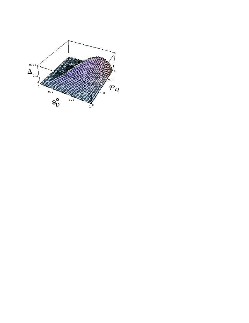
Figure 3: Difference $\Delta$ between the squares of the upper bounds of the visibility as a function of the norm of the Bloch vector $|\bm{s}_{D}^{(0)}|$ and the quanton predictability $\mathcal{P}_{Q}$. The plot is taken for a balanced detecton $\mathcal{P}_{D}=0$ coupled maximally to the quanton ($\mathcal{Q}=|\bm{s}_{D}^{(0)}|$).

As can be seen in the plot $\Delta=0$ for pure-state preparation ($|\bm{s}_{D}^{(0)}|=1$), since in this limit $\Xi$ always equals $\mathcal{D}$. The opposite limit of a totally unpolarized detecton ($|\bm{s}_{D}^{(0)}|=0$) leads to the limit of “bad” WWM ($\mathcal{Q}=0$) and $\Xi=\mathcal{D}$ since both quantities equal $\mathcal{P}_{Q}$. Conversely, for $\mathcal{P}_{\text{Q}}=0$ we have $\Xi=\mathcal{D}$ since both quantities equal $\mathcal{Q}$. This reciprocity stems from the symmetric structure of the right-hand side of Eq. (53) which yields $\mathcal{P}_{Q}$ ($\mathcal{Q}$) when $\mathcal{Q}$ ($\mathcal{P}_{Q}$) vanish. Thus, there is only deviation $\Delta\neq 0$ for unbalanced quanton interferometers ($\mathcal{P}_{Q}\neq 0$) and mixed state preparation. Finally, $\mathcal{P}_{Q}=1$ gives $\Xi=\mathcal{D}=1$ and the interference fringes are totally degraded so $\Delta=0$. In between, $\Delta$ can increase up to 0.25 for $\mathcal{P}_{Q}=\mathcal{Q}=|\bm{s}_{D}^{(0)}|=0.7$.

We have proved the right hand side of Eq. (48). Now we check the left-hand side. The quanton visibility is given in Eq. (57) of Jesus04 as

$$\mathcal{V}_{Q}=\mathcal{V}_{Q}^{o}\,\sqrt{\cos^{2}\Phi+\mathcal{P}_{D}^{2}\sin^{2}\Phi}.$$ (57)

Squaring and summing the above equation with Eq. (52) we have

$$\mathcal{Q}_{D}^{2}+\frac{\mathcal{V}_{Q}^{2}}{\mathcal{V}_{Q}^{o2}}=|\bm{s}_{D}^{o}|^{2}\sin^{2}\Phi+\cos^{2}\Phi\leq 1,$$ (58)

Now multiply Eq. (58) by $(1-\mathcal{P}_{Q}^{2})$ and simplify using Eqs. (51) and (53). We obtain

$$\mathcal{V}_{Q}^{2}+\Xi_{Q}^{2}\leq 1,$$ (59)

as we wanted to show.

This simple system illustrates different scenarios for Eq. (48). First take $\mathcal{P}_{D}=0$. Then, according to Eqs. (50) and (52), $\mathcal{Q}_{D}$ is proportional to the initial purity of the WWM given by the length of its Bloch vector, while $\mathcal{V}_{Q}/\mathcal{V}_{Q}^{o}$ depends only on the entangling phase. Lowering the initial purity of the WWM degrades the WWM’s ability to store WWI about the quanton. This action keeps $\mathcal{V}_{Q}$ unchanged but lowers both $\mathcal{D}_{Q}$ and $\Xi_{Q}$. Moreover, $\mathcal{D}_{Q}$ is lowered more than $\Xi_{Q}$, as can be seen by comparison of Eqs. (53) and (55), which yields $\mathcal{V}\leq\mathcal{V}_{\Xi}\leq\mathcal{V}_{\mathcal{D}}$. Now take $\mathcal{V}_{D}^{o}$ constant and $\mathcal{P}_{D}\neq 0$, so degrading the purity corresponds to lowering $\mathcal{P}_{D}$. In this case, this action keeps $\mathcal{Q}_{D}$ unchanged, but degrades $\mathcal{V}_{Q}/\mathcal{V}_{Q}^{o}$. Since $\mathcal{Q}_{D}$ and $\mathcal{P}_{Q}$ stay constant $\Xi_{Q}$ remains invariant, as can be seen from Eq. (53). However, $\mathcal{D}_{Q}$ degrades for $\mathcal{R}_{Q}\geq\mathcal{P}_{Q}$ since its value depends in this case explicitly on the value of the WWM’s purity, as can be seen from Eq. (55). The condition $\mathcal{V}\leq\mathcal{V}_{\Xi}\leq\mathcal{V}_{\mathcal{D}}$ is recovered, as can be seen in Fig. 4. Again, a maximum value of $\Delta=\mathcal{V}_{\mathcal{D}}^{2}-\mathcal{V}_{\Xi}^{2}=0.25$ can be obtained as in the previous case of the balanced detecton situation.

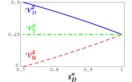
Figure 4: $\mathcal{V}_{\text{D}}^{2}$ (solid line), $\mathcal{V}_{\Xi}^{2}$ (dot-dashed line), and $\mathcal{V}_{\text{Q}}^{2}$ (thin dashed line) as a function of the detecton’s initial purity $|\bm{s}_{D}^{(0)}|$. The plot is taken for $\mathcal{V}_{\text{D}}^{o2}=\mathcal{P}_{\text{Q}}^{2}=0.5$ and a maximum entangling phase $\Phi=\pi/2$.

VI CONCLUSION

$\mathcal{V}^{2}+\Xi^{2}\leq 1$, like Eq. (1), is an inequality quantifying duality. Like Eq. (1), it devolves the same extreme cases given in Eqs. (41) which constitutes the usual statements about duality, i.e., concerning full WWI and no fringe visibility (particlelike aspects), or perfect fringe visibility and no WWI (wavelike aspects). In addition, both inequalities also quantify intermediate situations (not specified by the duality principle) where only partial WWI and partial fringe visibility are possible. In these situations the two inequalities yields two upper bounds for the visibility $\mathcal{V}_{\Xi}$ and $\mathcal{V}_{\mathcal{D}}$. For balanced interferometers ($\mathcal{P}=0$) $\mathcal{V}_{\Xi}=\mathcal{V}_{\mathcal{D}}$, since in this case $\Xi=\mathcal{Q}=\mathcal{D}$. For pure states, we also find that both visibility bounds coincide. However, for mixed states and unbalanced interferometers we obtain a remarkable result. We find that the visibility bound $\mathcal{V}_{\Xi}$ can be lower than $\mathcal{V}_{\mathcal{D}}$. Thus, $\mathcal{V}^{2}+\Xi^{2}\leq 1$ can be more stringent than $\mathcal{V}^{2}+\mathcal{D}^{2}\leq 1$.

Note that $\mathcal{D}$ is the largest possible value of the different knowledge $\mathcal{K}_{W}$ associated with a concrete betting strategy Englert96 ; Englert99 . Thus, $\mathcal{V}_{\mathcal{D}}$ in Eq. (46) is just the lowest upper bound to the visibility from all the bounds $\sqrt{1-\mathcal{K}_{W}^{2}}$ associated with different measurement choices of WWM’s observables $W$. On the other hand, since $\mathcal{V}\leq\mathcal{V}_{\mathcal{D}}$ does not saturate for mixed-state preparation, lower minima such as $\mathcal{V}_{\Xi}$ can still be found. The bound $\mathcal{V}_{\Xi}$ is not associated in general with the betting strategy mentioned before. Nevertheless, like $\mathcal{V}_{\mathcal{D}}$, $\mathcal{V}_{\Xi}$ is a manifestation of the quantum correlations established between the quanton and the WWM, derived through the algebraic properties of their Hilbert space.

We have particularized the results to a concrete example: the symmetric quanton-detecton system, which illustrates the different quantities introduced in the formalism. The inequalities $\mathcal{V}\leq\mathcal{V}_{\Xi}\leq\mathcal{V}_{\mathcal{D}}$ are shown to hold for this particular system. Actually, the difference between the visibility limits $\mathcal{V}_{\Xi}^{2}$ and $\mathcal{V}_{\mathcal{D}}^{2}$ in this system is significant and can reach a value of 0.25.

*

Appendix A

Here we show the connection between Eqs. (56) and the more general expression given in Eq. (43). In order to do that, consider the mixed state

$$\rho_{D}^{0}=D_{1}|\uparrow\rangle\langle\uparrow|+D_{2}|\downarrow\rangle\langle\downarrow|,$$ (60)

where

$$D_{1,2}=\frac{1}{2}(1\pm S_{Dz}^{0}),$$ (61)

and $\{|\uparrow\rangle,|\downarrow\rangle\}$ are the usual eigenvectors of $\sigma_{Dz}$. The quantity $\chi=\mathcal{D}^{2}/\Xi^{2}$ can be written in terms of $\Delta$ as

$$\chi=1-\frac{\Delta}{\Xi^{2}}.$$ (62)

With the help of the three previous equations, Eqs. (56) can be written

$$\chi=$$ {

,

.

which coincides with Eq. (43).

References

- (1) R. Feynman, R. Leighton, and M. Sands, The Feynman Lectures on Physics (Addison Wesley, Reading, MA, 1965), Vol. III.
- (2) Quantum Theory and Measurement, edited by J.A. Wheeler and W.H. Zurek (Princeton University Press, Princeton, NJ, 1983).
- (3) W.K. Wootters and W.H. Zurek, Phys. Rev. D 19, 473 (1979); R. Glauber, Ann. N.Y. Acad. Sci. 480, 336 (1986); D. Greenberger and A. Yasin, Phys. Lett. A128, 391 (1988); L. Mandel, Opt. Lett. 16, 1882 (1991).
- (4) G. Jaeger, A. Shimony, and L. Vaidman, Phys. Rev. A51, 54 (1995).
- (5) B.-G. Englert, Phys. Rev. Lett. 77, 2154 (1996).
- (6) G. Bjork and A. Karlsson, Phys. Rev. A 58, 3477 (1998).
- (7) B.-G. Englert and J. Bergou, Opt. Commun. 179, 337 (2000).
- (8) S. Durr, T. Nonn, and G. Rempe, Nature (London) 395, 33 (1998); S. Durr, T. Nonn, and G. Rempe, Phys. Rev. Lett. 81, 5705 (1998).
- (9) P.D.D. Schwindt, P.G. Kwiat, and B.-G. Englert, Phys. Rev. A 60, 4285 (1999).
- (10) S. Durr and G. Rempe, Opt. Commun. 179, 321 (2000).
- (11) J. Martinez-Linares and D.A. Harmin, Phys. Rev. A69, 062109 (2004).
- (12) P. Bertet, et al., Nature (London) 411, 166 (2001).
- (13) B.-G. Englert, Acta Phys. Slov. 46, 249 (1996).
- (14) As noted in Englert96b , there is no need to consider a more generic Bloch vector than that given in Eq. (5), since this just amounts to a redefinition of the operators in (6).
- (15) Or equivalently, after the BM.
- (16) We exclude the trivial case , where the three visibilities of Eq. (48) vanish.