A study of a local Monte Carlo technique for simulating systems of charged particles

Abstract

We study some aspects of a Monte Carlo method invented by Maggs and Rossetto for simulating systems of charged particles. It has the feature that the discretized electric field is updated locally when charges move. Results of simulations of the two dimensional one-component plasma are presented. Highly accurate results can be obtained very efficiently using this lattice method over a large temperature range. The method differs from global methods in having additional degrees of freedom which leads to the question of how a faster method can result. We argue that efficient sampling depends on charge mobility and find that the mobility is close to maximum for a low rate of independent plaquette updates for intermediate temperatures. We present a simple model to account for this behavior. We also report on the role of uniform electric field sampling using this method.

I Introduction

As an aid to understanding the behavior of statistical systems, it is common practice to carry out computer simulations of models that are invented to capture the physical behavior of interest because, even for unelaborate models, it is often extremely difficult to find approximate and especially exact analytical results. Both Monte Carlo and molecular dynamics methods work by generating large numbers of particle or field configurations from which correlation functions can be obtained that converge to thermal averages by design. In Monte Carlo, each new configuration is produced by making a pseudorandom change to the last one in the chain, testing the ratio of Boltzmann weights (which, in the canonical ensemble, amounts to a computation of the energy difference), and choosing either the new configuration or the old one. Molecular dynamics is a numerical evolution of a many-body system from the equations of motion of the component ’particles’ with some constraint depending on the ensemble - for example to maintain a constant temperature. The degree of approximation to thermal equilibrium in both cases is limited, in practice, by the efficiency with which the algorithm samples the regions of highest probability in the space of configurations, and the rate at which configurations can be produced. These two factors determine the range of system sizes that can be sampled effectively, though a compromise must often be made between obtaining large numbers of configurations based on the relaxation time of the combined model and algorithm and choosing large enough systems to lessen finite size effects that obscure the thermal equilibrium results required and which are usually poorly understood.

This work is a study of a Monte Carlo technique for simulating systems of thermalized classical charges. Most of the systems studied in soft condensed matter laboratories fall into this class. It includes simple liquids, polymers, colloids, liquid crystals, proteins and other biologically active molecules.

In many interesting cases, charged particle interactions can be screened by the charges themselves, giving an effective interaction of the Yukawa form with a screening length that can often be tuned in experiments. But there are also many cases where one must consider the exact Coulomb interaction. Because the Coulomb interaction is long-ranged, one must presumably either compute all pairwise interactions with the charge that is moved at a given step (in Monte Carlo) or one must solve the Poisson equation at each step. Consider a Monte Carlo simulation with $N$ charges. When a charge is moved, the energy difference between configurations requires $O(N)$ operations for all pairwise interactions. Each Monte Carlo sweep, which is defined to be $N$ charge moves or Monte Carlo steps, requires $O(N^{2})$ operations; this is how the simulation will slow down as the system size increases. With short range interactions, in contrast, we expect $O(N)$ operations for each sweep.

The order $O(N^{2})$ scaling for Coulomb interactions is a real problem and a great deal of effort has been devoted to improving the scaling and the prefactor that accompanies it. This study focuses on a relatively new method proposed by Maggs and Rossetto RossettoMaggs , which achieves $O(N)$ scaling and which has some promise as a competitive approach for simulating charged particles using either molecular dynamics or Monte Carlo.

I.1 Local Electrostatics

The gist of the method of Maggs and Rossetto is as follows. Rather than solving the Poisson equation (which follows from Gauss’ law supplemented with the condition that the electric field circulation vanish) at each step, one imposes only Gauss’ law. The electric field circulation decouples from the charges, so it averages out during the simulation and one obtains electrostatic averages. Gauss’ law can be imposed locally in the sense that when a charge moves, this divergence condition can be maintained by changing the electric field in the neighborhood of the charge only. Transposing this result to Monte Carlo, we see that each sweep requires only $O(N)$ operations.

Now we fill in details of the argument RossettoMaggs . Consider a number of charged particles with charge density $\rho(\mathbf{r})=\sum_{i}q_{i}\delta(\mathbf{r}-\mathbf{r}_{i})$. Suppose the electric field $\mathbf{E}$ is affected by the charge distribution only to the extent that Gauss’ law is satisfied

$$\mathbf{\nabla}\cdot\mathbf{E}=\rho(\mathbf{r}).$$

In other words we do not impose the further condition required for electrostatics that the curl of the electric field be equal to zero. The charged particle system is closed so that the amount of charge does not change and the whole system is immersed in a heat bath at inverse temperature $\beta$. The partition function in this canonical ensemble in two dimensions is

$$Z(\beta)=\int\prod_{i}d^{2}\mathbf{r}_{i}\int\mathcal{D}\mathbf{E}\,\delta(\mathbf{\nabla}\cdot\mathbf{E}-\rho(\mathbf{r}))\\ \times\exp\left(-\frac{\beta}{2}\int d^{2}\mathbf{r}\,\mathbf{E}^{2}(\mathbf{r})\right),$$ (1)

in which the factor resulting from the momentum integration over each particle has been left out. The electric field can be split into an irrotational or longitudinal part $\mathbf{E}_{\|}$ and a transverse part $\mathbf{E}_{\bot}$: $\mathbf{E}=\mathbf{E}_{\|}+\mathbf{E}_{\bot}$ satisfying

$$\begin{array}[]{ccc}\mathbf{\nabla}\cdot\mathbf{E}_{\bot}=0&\mbox{and}&\mathbf{\nabla}\times\mathbf{E}_{\|}=0.\end{array}$$

Gauss’s law can now be written as $\mathbf{\nabla}\cdot\mathbf{E}_{\|}=\rho(\mathbf{r})$ and with the condition on the longitudinal field that its curl vanish, $\mathbf{E}_{\|}$ is derivable from a scalar field $\phi(\mathbf{r})$ which obeys Poisson’s equation

$$\nabla^{2}\phi(\mathbf{r})=-\rho(\mathbf{r})$$

$$\mathbf{E}_{\|}=-\mathbf{\nabla}\phi(\mathbf{r}).$$

The solution to the Poisson equation in two dimensions is uniquely

$$\phi(\mathbf{r})=-\frac{1}{2\pi}\int d^{2}\mathbf{r}^{\prime}\rho(\mathbf{r}^{\prime})\ln|\mathbf{r}-\mathbf{r}^{\prime}|.$$

We return to the energy functional to see the effect of separating out the longitudinal and transverse contributions

$$\int d^{2}\mathbf{r}\,\mathbf{E}^{2}(\mathbf{r})=\int d^{2}\mathbf{r}\left[(\mathbf{\nabla}\phi)^{2}+\mathbf{E}_{\bot}^{2}-2\mathbf{\nabla}\phi\cdot\mathbf{E}_{\bot}\right].$$

Partially integrating the third term, we get

$$2\int d^{2}\mathbf{r}\,\phi(\mathbf{\nabla}\cdot\mathbf{E}_{\bot})=0.$$

The whole of the dependence of the energy on the charge positions is contained in the scalar potential so the partition function factorizes:

$$Z(\beta)=Z_{\mathbf{E}_{\bot}}(\beta)\times\int\prod_{i}d^{2}\mathbf{r}_{i}\,\exp\left(-\frac{\beta}{2}\int d^{2}\mathbf{r}\,(\mathbf{\nabla}\phi)^{2}\right)$$

where $Z_{\mathbf{E}_{\bot}}(\beta)$, which comes from the Gaussian integration over the transverse degrees of freedom, is independent of the charge configuration. So thermodynamic averages derived from the partition function (1) are the same as those that would be found from the partition function with the electrostatic energy functional.

Because Gauss’ law can be imposed locally, we ought to be able to run Monte Carlo simulations of systems of charged particles with local field updates and hence local energy computations at each step rather than solving Poisson’s equation to find the new unique global field configuration for each charge configuration. The advantage of having local energy computations at each step is an improvement in the scaling of the algorithm over methods involving direct evaluation of the pairwise interaction. Each particle move is a local operation involving $O(1)$ operations, so the scaling of the time per Monte Carlo sweep is $O(N)$. The transverse field must also be sampled, and yet one finds that this does not contribute significantly to the scaling. This latter fact is quite counterintuitive and we shall devote some more attention to it in the following.

It is worth pointing out that if we begin with Maxwell’s electrodynamics, a similar argument to the one given above shows that electrostatic averages follow in this case. This is not remarkable given the decoupling of the divergence and circulation of the electric field in the pure electric field case described above, but we set out this result in an appendix. One could therefore devise a molecular dynamics algorithm with the appropriate constraint for working at constant temperature that integrates Maxwell’s equations (which are local equations) at each time-step and with the speed of light as a variable, chosen to be small enough so that the algorithm is truly local, and obtain the same results that would be obtained directly from electrostatics. However, Maggs and Rossetto have shown that one is free to find the simplest local dynamics possible for the charges that simultaneously samples longitudinal and transverse degrees of freedom subject to Gauss’ law, and use this dynamics to perform much more efficient Monte Carlo or molecular dynamics simulations than would be possible with full Maxwell electrodynamics. In this paper, we shall use a charge and field dynamics invented by Rottler and Maggs RottlerMaggs that omits magnetic fields altogether.

I.2 Overview

In the next section, we provide a very short introduction to charge interactions in periodic media in the continuum limit and for the case where the electric field is discretized onto a lattice. Hence, we describe the conventional $O(N^{2})$ global Monte Carlo method we have used and give a practical account of the corrections that must be made to lattice simulations to better approximate the continuum pair-wise potential. Section III describes the implementation of the local $O(N)$ method for Monte Carlo simulations with charges moving off-lattice with particular attention to unusual features of the dynamics; I also present a continuum version of the local update method which shows some already known features very transparently. Global and local Monte Carlo methods are applied in Section IV.2 to the 2D OCP and we discuss the accuracy of the local methods and the effect of uniform field sampling. Then, we shall see that charge autocorrelation times are much greater for the local method than for global methods. Section IV.4 includes the autocorrelation data into a comparison of the speeds of the local method and a global method for typical system sizes. Results of an investigation into the effects of the transverse electric field on charge relaxation times are given in Section IV.5. We also discuss the problem of how additional degrees of freedom result in $O(N)$ scaling when the naive expectation is that transverse fields should be allowed to relax across the system at each step. The first appendix derives a useful result for corrections to 2D lattice-based simulations. The second appendix shows that the argument of Maggs and Rossetto given above carries over to Maxwell electrodynamics.

II Simulation methods

The Monte Carlo simulations that will be discussed below are based on the acceptance procedure of Metropolis and co-workers Metropolis . This involves the computation of a difference in energies of two field configurations at each step. The simulation methods we have used are distinguished by the ways in which this difference is found.

In this section, we discuss the interactions between charged particles in rectangular cells with periodic boundary conditions and the corrections that have to be made to the interaction when the electric field is put onto a lattice in order to better approximate the continuum potential energy. We describe the simulation methods we have used in turn, starting with the continuum case, then the problems of discretization, and leaving the special properties of the local algorithm until the next section. In the following, unless otherwise stated, we consider two dimensional electrostatics for notational simplicity and because this is most appropriate to the simulations that we have performed.

II.1 Periodic systems

The potential energy of a finite number of charges in a rectangular cell with periodic boundary conditions is a conditionally convergent series over all pairwise Coulomb energies for the charges in the infinite array of cells implied by the boundary conditions. Each cell must be charge neutral otherwise the series is divergent. And if the dipole moment in each cell is zero the sum is absolutely convergent. In general, the dipole moment in each cell is non-vanishing, so the problem is to devise a physically motivated summation of the series. A further problem is to identify the unique solution to the Poisson equation with periodic boundary conditions. These have been solved by Leeuw and Perram Leeuw2 by obtaining the potential for a large spherical cluster of identical cells embedded in a medium of dielectric constant $\epsilon$; their expression includes a term that depends on the net dipole moment of the elementary cell and the dielectric constant of the surrounding medium. The unique periodic solution to the Poisson equation is obtained in the limit as $\epsilon\rightarrow\infty$ and corresponds to the case of a large spherical cluster of identical rectangular cells of charges surrounded by a perfect conductor that perfectly cancels the dipole moment of the cluster of cells Fraser . The periodic potential, called the Ewald potential, ((13) given in the first appendix for the two dimensional case Leeuw2 ) is a pairwise potential for charges in a rectangular box that includes the direct Coulomb potential and also the potential due to all the image charges for the pair considered. The dipole moment term that is present for finite $\epsilon$ takes the form

$$U_{\mbox{dip}}=\frac{\pi}{2L_{x}L_{y}(\epsilon+1)}\left(\sum_{a=1}^{N}q_{a}\mathbf{r}_{a}\right)^{2}$$ (2)

for cell lengths $L_{x}$ and $L_{y}$ and with charge $q_{a}$ at position $\mathbf{r}_{a}$. This will be discussed further in connection with the local method.

The Ewald potential splits the calculation of the potential into short-range and long-range parts. The latter is performed in Fourier space. This forms the basis for molecular dynamics simulations. However, the Ewald potential is not always the most efficient starting point for computations. I have used the form found by Lekner Lekner1 ; Lekner2 and developed for rectangular periodic cells by Grønbech-Jensen GronJen . If the charges are separated by a vector with Cartesian components $x$ and $y$ and the cell lengths are, once again, $L_{x}$ and $L_{y}$, then the pairwise potential energy between unit charges is

$$2\pi V=K\left(\frac{L_{y}}{L_{x}}\right)+\frac{\pi L_{y}}{L_{x}}\left(\frac{y}{L_{y}}\right)^{2}\\ -\frac{1}{2}\ln\left\{\prod_{k=-\infty}^{\infty}\frac{\cosh\left(2\pi\frac{L_{y}}{L_{x}}\left(\frac{y}{L_{y}}+k\right)\right)-\cos\left(\frac{2\pi x}{L_{x}}\right)}{\cosh\left(2\pi\frac{L_{y}}{L_{x}}k\right)}\right\}$$ (3)

where $K$ is a constant that includes the interaction of the charges with the uniform background charge and with all their image charges and is given by

$$K\left(\frac{L_{y}}{L_{x}}\right)=\frac{\pi}{6}\frac{L_{y}}{L_{x}}-\frac{1}{2}\ln 2-\ln\prod_{k=1}^{\infty}\left(1+\exp\left(-4\pi\frac{L_{y}}{L_{x}}k\right)\right).$$

The advantage of this formula is that it is in terms of elementary functions; although it is an infinite product in its main part, the product converges very quickly - I take $|k|\leq 5$ which agrees with the exact result to machine precision.

II.2 Lattice simulations

The $O(N)$ Monte Carlo method that is the subject of this paper requires that we discretize the electric field so that it lives on the links of a square mesh with charges on the sites. Overall charge neutrality must be maintained (if necessary by having a uniform background charge). We consider the case of a two-dimensional square lattice with lattice spacing $a$, site labels $\{\mathbf{R}\equiv(n_{x},n_{y})\}$ and link directions $\mu=x,y$ such that charge $q(\mathbf{R})$ is assigned (in the way described above) to site $\mathbf{R}$ and electric fields are defined on the links of the lattice with $E(\mathbf{R},-\mu)=-E(\mathbf{R}-\mu,\mu)$ by convention. The lattice has $N_{x}=L_{x}/a$, $N_{y}=L_{y}/a$ plaquettes in the $x$ and $y$ directions respectively. Sites $n_{x}=0$ and $n_{x}=N_{x}$ are identified. Periodicity in the $y$ direction is implemented in the same way.

The discrete form of Gauss’ law is

$$\sum_{\mu=x,y}a(E(\mathbf{R},\mu)+E(\mathbf{R},-\mu))=q(\mathbf{R}).$$ (4)

When the Poisson equation is discretized onto the lattice, its solution can be written as

$$\phi(\mathbf{R})=\sum_{\mathbf{R}^{\prime}}G(\mathbf{R}-\mathbf{R}^{\prime})q(\mathbf{R}^{\prime}).$$

The charge at lattice site $\mathbf{R}$ is $q(\mathbf{R})$ and $G(\mathbf{R})=G(n_{x},n_{y})$ is the lattice Green’s function. One can show, by calculating the discrete Fourier transform of the Poisson equation with periodic boundary conditions, that

$$G(n_{x},n_{y})=\sum_{p_{x}=0}^{N_{x}-1}\exp\left(2\pi i\frac{p_{x}n_{x}}{N_{x}}\right)\sum_{p_{y}=0}^{N_{y}-1}\exp\left(2\pi i\frac{p_{y}n_{y}}{N_{y}}\right)\\ \times\frac{1}{N_{x}N_{y}}\frac{1}{4-2\cos(\frac{2\pi p_{x}}{N_{x}})-2\cos(\frac{2\pi p_{y}}{N_{y}})}$$ (5)

in two dimensions. The electric field is related to the potential on the lattice by $aE_{x}(n_{x},n_{y})=\phi(n_{x}+1,n_{y})-\phi(n_{x},n_{y})$ and similarly for the $y$ component.

The charged particles are not confined to the lattice sites in our simulations. In common with most molecular dynamics simulations of charged particles, charges are smoothly assigned to lattice sites in the neighborhood of each particle as a function of the particle position. Suppose that each charge $q_{a}$ at continuous position $\mathbf{r}_{a}$ is spread over lattice sites $\{\mathbf{R}_{i}\}$. The charge on site $\mathbf{R}_{k}$ is given by $q_{a}s(\mathbf{r}_{a},\mathbf{R}_{k})$. We call $s$ the charge assignment function which has the property

$$\sum_{j}s(\mathbf{r}_{a},\mathbf{R}_{j})=1.$$

Many choices of assignment function are possible and the choice may greatly affect the performance of the algorithm. Clearly, as the number of lattice sites over which each charge is distributed increases, the computational cost increases also. As for the accuracy, the overlap of lattice based charge clouds results in a deviation from the continuum potential for charge separations on the scale of the charge cloud. Because, for high accuracy, one should correct the energy for charges with overlapping charge clouds, there is a greater computational cost for higher order assignment functions. For Fourier transform methods, including most molecular dynamics methods Mesh , accuracy can increase as the radius of the charge cloud increases. This is because narrow charge clouds have a large spread in Fourier space and higher frequency modes can act as aliases for lower frequency ones in the sense that modes of different frequency can appear the same on the scale of the lattice if their values at the lattice sites coincide. To avoid this aliasing error, it is better, for these simulation methods, to have larger charge clouds so that frequency aliases have a smaller amplitude. We use a third order scheme due to Hockney and Eastwood HandE that spreads the charges over nine vertices in two dimensions. If $Dx$ and $Dy$ are the distances in units of the lattice spacing $a$ of the charge $q$ to the vertex $v_{0,0}$ closest to it, the weights for charge assignment in the $x$ direction are

$$\begin{array}[]{c}W^{x}_{-1}=(Dx-0.5)^{2}/2\\ W^{x}_{0}=0.75-Dx^{2}\\ W^{x}_{+1}=(Dx+0.5)^{2}/2\end{array}$$ (6)

with similar formulas for the $y$ direction assignment. The charge assignment function $s$ is a product of pairs of weights as shown in Figure 1.

The total energy of the system in terms of the Green’s function is

$$U=\frac{1}{2}\sum_{\mathbf{r}_{a}}\sum_{\mathbf{r}_{b}}\sum_{i,j}q^{2}G(\mathbf{R}_{i}-\mathbf{R}_{j})s(\mathbf{r}_{a},\mathbf{R}_{i})s(\mathbf{r}_{b},\mathbf{R}_{j}).$$ (7)

Alternatively, it is the sum of all the squared link electric fields

$$U=\frac{a^{2}}{2}\sum_{n_{x}=0}^{N_{x}-1}\sum_{n_{y}=0}^{N_{y}-1}\left(E^{2}((n_{x},n_{y}),x)+E^{2}((n_{x},n_{y}),y)\right).$$ (8)

This interaction is the one generated by the local simulation algorithm. At charge separations greater than about one lattice spacing (depending on the charge assignment scheme used) this interaction energy is an excellent approximation to the Ewald potential. At short range the interaction is weaker than in the continuum problem. In fact the limit of the interaction energy as the separation of two charges tends to zero is finite. For accurate simulation this must be corrected. For each charge move, charges in the neighborhood of the charge that is being moved are identified using the linked list method of Hockney and Eastwood HandE . The discretized interaction energy from equations (7) (with the sum suitably restricted) and (5) is subtracted off for each pair of neighboring charges and the Lekner potential $V$ from equation (3) or a good short range approximation to the Ewald potential is added on in its place. A suitable approximation for small charge separations $r$ is

$$U_{SRC}=-\dfrac{q^{2}}{2\pi}\ln r+\dfrac{q^{2}r^{2}}{4A}$$ (9)

where $A=L_{x}L_{y}$, which is derived in an appendix and presented with a calculation of the deviation from the Lekner potential for different charge separations. For very high accuracy or for low temperatures, the Lekner interaction is more appropriate. The linked list method is a local method so that the scaling of the local algorithm is preserved. The periodic cell is divided up into chaining cells - regions of $2\times 2$ plaquettes in our simulations. At the beginning of the simulation, the charges are given chaining cell labels and this information is put into a linked list. The linked list is composed of two arrays; the first gives a charge label given a chaining cell label - in other words it gives the label of one charge in a given chaining cell; the second array has particle labels as its contents and also as its indices in such a way that given a particle label, another particle in the same chaining cell is found using the previous element as an index, the new element being zero if there are no more charges in the chaining cell. For a more detailed explanation of this computer algorithm we refer to the book by Hockney and Eastwood HandE .

There is another problem associated with working on a lattice: the interaction includes finite self-energies for the charges: because each point charge is spread over several lattice sites, it interacts with itself with finite energy. The self-energy in this context is a one particle potential energy that has regular wells at positions relative to the lattice sites. This energy must be subtracted off, once again using (7) (with the sum taken over the sites over which each charge is spread) and (5). This subtraction is essential; without it, one finds that the charges become trapped within the lattice-induced potential wells at low temperatures, while higher temperature results are also strongly affected by this potential.

III Local method

III.1 Continuum update

The novelty of the local algorithm is in the way the field configuration changes. When a charge moves, the field changes in the vicinity of that charge so that Gauss’ law is preserved. We first consider charge moves in the continuum limit to illustrate some features of the dynamics. Because, in this subsection, we are not directly concerned with computations, we work with SI units and in three dimensions.

The electric field at time $t$ due to particle motion can be written as

$$\mathbf{E}(\mathbf{r},t)=\mathbf{E}(\mathbf{r},t_{0})-\sum_{i}\frac{q}{\epsilon_{0}}\int d\mathbf{r}_{i}\delta(\mathbf{r}-\mathbf{r}_{i}(t))$$

where $\mathbf{E}(\mathbf{r},t_{0})$ is the purely longitudinal electric field at time $t_{0}$ when the charges are in their starting positions. The electric field, according to this equation, evidently varies locally as the charges move. Each charge leaves a trail along its path as pointed out by Levrel and Maggs LevrelMaggs . If we take any closed surface around some charges at $t_{0}$, Gauss’ law is satisfied by the definition of $\mathbf{E}(\mathbf{r},t_{0})$. As time increases, charges may enter or leave this closed surface, whereupon the delta function ensures that flux is chopped out or added in at the cutting point to preserve Gauss’ law. If $F$ is the closed surface

$$-\frac{q}{\epsilon_{0}}\oint_{F}d\mathbf{S}\cdot\int d\mathbf{r}_{i}\delta(\mathbf{r}-\mathbf{r}_{i}(t))\\ =\left\{\begin{array}[]{ll}\pm q/\epsilon_{0}&\mbox{if the charge cuts $F$ an odd number of times}\\ 0&\mbox{otherwise}\end{array}\right.$$

where the sign on the right-hand-side depends on whether the charge is originally inside (minus sign) or outside $F$. The electric field trail term can be written as

$$-\sum_{i}\frac{q}{4\pi\epsilon_{0}}\int d\mathbf{r}_{i}\nabla^{2}\left(\frac{1}{|\mathbf{r}-\mathbf{r}_{i}(t)|}\right)$$

in three dimensions. Using the identity

$$\nabla^{2}\mathbf{V}=\mathbf{\nabla}(\mathbf{\nabla}\cdot\mathbf{V})-\nabla\times\nabla\times\mathbf{V}$$

for vector field $\mathbf{V}$ we notice that, in accordance with the Helmholtz theorem, the electric field can be split into longitudinal and transverse parts

$$\mathbf{E}=\mathbf{\nabla}\phi+\mathbf{\nabla}\times\mathbf{Q}$$

where

$$\phi(\mathbf{r})=\sum_{i}\frac{q}{4\pi\epsilon_{0}}\mathbf{\nabla}\cdot\int d\mathbf{r}_{i}\left(\frac{1}{|\mathbf{r}-\mathbf{r}_{i}(t)|}\right)+\phi(\left\{\mathbf{r}_{i}(t_{0})\right\})$$

and

$$\mathbf{Q}=\sum_{i}\frac{q}{4\pi\epsilon_{0}}\mathbf{\nabla}\times\int d\mathbf{r}_{i}\left(\frac{1}{|\mathbf{r}-\mathbf{r}_{i}(t)|}\right).$$

We can go further and write the scalar and vector potentials as

$$\phi(\mathbf{r})=\sum_{i}\frac{q}{4\pi\epsilon_{0}}\int\frac{d\mathbf{r}_{i}\cdot(\mathbf{r}-\mathbf{r}_{i}(t))}{|\mathbf{r}-\mathbf{r}_{i}(t)|^{3}}\\ =\sum_{i}\frac{q}{4\pi\epsilon_{0}}\int d\mathbf{r}_{i}\cdot\mathbf{\nabla}_{i}\left(\frac{1}{|\mathbf{r}-\mathbf{r}_{i}|}\right)+\phi(\left\{\mathbf{r}_{i}(t_{0})\right\})$$

which is recognizable is the ordinary electric scalar potential while

$$\mathbf{Q}=\sum_{i}\frac{q}{4\pi\epsilon_{0}}\int\frac{d\mathbf{r}_{i}\times(\mathbf{r}-\mathbf{r}_{i}(t))}{|\mathbf{r}-\mathbf{r}_{i}(t)|^{3}}$$

which is the Biot-Savart law. So, the electric field at each time $t$ is the Coulomb field due to the charges at time $t$ positions, and a circulation $\mathbf{\nabla}\times{\mathbf{Q}}$ where $\mathbf{\mathbf{Q}}$ is equivalent to the magnetic field produced by current-carrying wires along the trails left by the charges as they move - the current being $q/\mu_{0}\epsilon_{0}$.

We notice that if a charge makes a closed loop, there is no change in the longitudinal field as we should expect. Secondly, the transverse field is always zero for the closed loop except on the loop itself, in accordance with $\mathbf{\nabla}\times{\mathbf{Q}}$ being proportional to the current density in ordinary electromagnetism. When the path is not closed, this relationship breaks down; in terms of the current-carrying wires analogy, the endpoints imply that charge is not conserved so there is an additional magnetic field contribution, the curl of which is identical to the Coulomb field of the charge at the endpoints. We have demonstrated, that pure transverse field updates occur entirely by the motion of charges in closed loops.

III.2 Off-lattice charge move update

The O(N) Monte Carlo charge update requires us to maintain the discretized version of Gauss’ law, equation (4), at each charge move by changing a few links as possible for a given charge assignment function. The energy difference computation at each step from equation (8) involves only the link fields that have changed. There are many possible ways of updating the electric field locally. When charges are completely confined to the lattice sites, then hopping of charge $q$ across a link requires us to alter the electric field $E$ on that link by $E\rightarrow E-q/a$ to preserve the flux constraint. The charge leaves a trail of electric field, as we have already seen in the continuum case. I have used the following field update procedure for off-lattice simulations RossettoMaggs . Given the restrictions on charge motion and the assignment function, the number of vertices affected by the charge move must be either nine or twelve. Suppose that the nearest vertex to the charge $\mathbf{R}_{0}$ is the same before and after the move so that only nine vertices are affected; the other case is identical in principle. For each affected vertex $\mathbf{R}(p,q)\equiv\mathbf{R}_{0}+p\mathbf{x}+q\mathbf{y}$ with $p,q=-1,0,1$, the change in the charge is $\Delta q(\mathbf{R}(p,q))$. Beginning at the vertex $\mathbf{R}(-1,-1)$, we trace out an $S$ shape, updating the links along the path so that, at each site along the path, Gauss’ law is satisfied. Figure 1 shows the general idea.

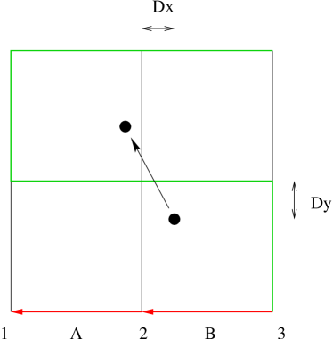
Figure 1: Charge update for charge move in neighborhood of a single plaquette. Completed link updates are shown in red. Those to be updated in green. The original charge position from the nearest vertex is given by $Dx$ and $Dy$ and the charge assignments on vertices $1$,$2$ and $3$ are initially given by $W^{y}_{-1}W^{x}_{-1}$, $W^{y}_{-1}W^{x}_{0}$ and $W^{y}_{-1}W^{x}_{1}$ respectively where the charge assignment weights $W$ are given in equation (6). If, when the charge moves, the change on vertex $i$ is $\Delta q(i)$ then the link field denoted A is updated by $E_{A}\rightarrow E_{A}+(\Delta q(1)/a)$ and for link B $E_{B}\rightarrow E_{B}+((\Delta q(1)+\Delta q(2))/a)$ and so on.

III.3 Other features

In continuum terms, the local update is responsible for generating an electric field of the form

$$\mathbf{E}=-\mathbf{\nabla}\phi+\mathbf{\nabla}\times\mathbf{Q}+\mathbf{E}_{b}$$ (10)

with $\mathbf{Q}$ and uniform field $\mathbf{E}_{b}$ non-vanishing at finite temperature. By definition, the potential produces an electric field with no net background field $\mathbf{E}_{b}$, but the local field update gives rise to fluctuations in this field. To see this, consider a charge that hops from one lattice site to a neighboring site. The simplest local field update produces a field trail that would restore the charge to its original position at zero temperature. If the uniform background were zero before the charge hopped between sites, then because the background field is the sum over the vectors at each site divided by the total number of links there must such a field in the final state. This field can be spread over the lattice by further field updates. From this kind of argument, we see that the background field that is generated depends on the distance of the charges from their original positions. More precisely, at time $t$, a single charge will be responsible for a uniform electric field that is proportional to $q(\mathbf{r}(0)-\mathbf{r}(t))$ where $\mathbf{r}(0)$ is the original position of the charge $q$ and $\mathbf{r}(t)$ is its position at time $t$. It should be emphasized that $\mathbf{r}$ is measured without any regard for the periodicity of the cell. In other words, the electric field increases as a charge winds around the cell so the charge experiences a restoring force towards its original position. With many charges, the uniform field is proportional to $\sum_{i}q_{i}(\mathbf{r_{i}}(0)-\mathbf{r_{i}}(t))$. So we should expect that fluctuations in the uniform field will cause charges to lose sense of their original positions.

It has been argued that the local update can produce, even after averaging, an interaction of the more general type considered by Leeuw and Perram - a periodic potential and a term that depends on the dipole moment of the cell RottlerMaggs and which is equivalent to the presence of a uniform electric field within the cell. We recall from Section II that the periodic interaction is recovered from a spherical cluster of identical cells by cladding the cluster with a perfect conductor. If the cladding has finite dielectric constant $\epsilon$, a dipole term is introduced as in equation (2). The dipole term in the cell is bounded because the cell is finite. In contrast, the uniform field produced by the local is unbounded and does not depend on the absolute dipole moment unless the dipole moment of the cell is zero at the beginning of the simulation. The argument RottlerMaggs is that at high temperatures, charge winding causes the uniform electric field to average out during the simulation. At low temperatures though, the field does make a difference to the effective interaction after thermally averaging.

One can see that the uniform field makes no difference to thermal averages provided it is sampled independently of charge positions. So one way of ensuring infinite $\epsilon$ is to introduce an independent background field update. This can be implemented locally. It has the disadvantage of slowing the simulation down. A more efficient means is to keep track of the uniform field locally and to subtract off its contribution to the energy. This can be done because the uniform field energy decouples from other contributions even before thermal averaging. We shall investigate the influence of the uniform field further in the next section.

Although charge updates do sample transverse electric field configurations, we expect to have to sample these circulations independently of the charge moves. For the circulation sampling, a plaquette is chosen at random from a uniform distribution over the whole lattice. A number $\Delta$ is then selected from a uniform distribution over the range $[-\nu,\nu]$ where $\nu$ is chosen so that the move has a $50\%$ acceptance rate. The circulation of the electric field around the chosen plaquette is changed by altering each of the links of the plaquette by $\Delta$ as shown in figure 2. The energy difference calculation therefore involves only four link variables.

Figure 2: Plaquette circulation update at lattice site (ij). The electric field divergence at each site is preserved.

III.4 Literature

Monte Carlo with O(N) scaling by the introduction of transverse field degrees of freedom may have charges confined to the lattice as introduced in RossettoMaggs ; LevrelMaggs , or allowed to move off-lattice with some smooth charge assignment onto the lattice vertices RottlerMaggs which we have followed in our simulations.

At first sight, we would expect that the transverse field degrees of freedom would have to be allowed to relax across the whole system for each particle move. Although the scaling of the speed varies as order $N$ when only particle moves are considered, one would naively expect order $N^{2}$ scaling when transverse field sampling is included. It turns out, however, Maggs1 that one can sample the transverse fields much less frequently than one would expect without spoiling the results. This is a surprising result. In connection with this issue, Maggs and coworkers Review have drawn attention to the fact that the transverse electric field is sampled by charge moves without requiring independent plaquette updates. In this paper we expand on this observation.

It has been found that for charges confined to a lattice, charges tend to freeze in their original positions. Two papers are devoted to various ways of removing this obstacle in on-lattice simulations LevrelMaggs ; Duncan by improving the efficiency of circulation updates or by spreading the charges over several sites. For off-lattice simulations, this problem can be present but one can avoid it by taking the step size to be small or by spreading charges over more sites.

The local update method has been developed by Maggs and collaborators for molecular dynamics RottlerMaggs2 ; Dunweg and in work by Pasichnyk and Dünweg Dunweg , the competitiveness of local molecular dynamics was remarked on in a comparison with a global $O(N)$ method.

The method has been applied in various test cases in the original papers. More recently however, it has been used by Maggs to carry out Monte Carlo simulations of a model of water Maggs2 .

IV Results of computer experiments

IV.1 The one-component plasma in two-dimensions.

Our simulations focus on the one-component plasma in two dimensions. This is a system of particles, all with charge $q$, on a fixed neutralizing background. In two dimensions the interaction between the charges is logarithmic. The phase diagram of this plasma depends only on the coupling $\Gamma$ where $2\pi\Gamma\equiv q^{2}\beta$. For $\Gamma=2$ the model can be solved exactly for the free energy and the $n$-point correlation functions. At around $\Gamma=140$, Monte Carlo simulations using periodic boundary conditions have revealed the existence of a first-order transition from a liquid to a crystalline phase. Most of the numerical work in the following focuses on this model. Firstly, the exact solution allows us to perform an objective test of the accuracy of the lattice based methods. Secondly, the plasma has long-ranged correlations for $\Gamma>2$ which form the basis for a stronger test of the achievable accuracies. Thirdly, the model has a simple formulation and is suitable for making clean tests of other properties of the new method including the effect of varying the rate of independent circulation updates.

IV.2 Simulations of the 2D OCP

I have carried out Monte Carlo simulations of the one-component plasma in two dimensions using the local electrostatic algorithm discussed at length in the previous section and also a continuum method using the Lekner form for the pairwise interaction. The simulation cell for the discrete methods is divided into $32\times 32$ plaquettes and each chaining cell is a $2\times 2$ plaquette region. The short range correction algorithm extends over a $6\times 6$ plaquette square with the charge that is moved in the central chaining cell. I used the approximation to the Lekner potential (9) as the correcting potential. All the results in this subsection were taken with $120$ charges in the simulation cell. The lattice spacing $a$ was chosen so that the number density of the particles was unity. The rate of plaquette updates was usually taken to be 40 for each charge move. Differences between the results obtained here and the correct thermal averages arise from small differences in the potential energy for small charge separations because an approximation to the correct potential is used (see appendix A) and also from imperfect sampling when the relaxation times are large which happens towards the lower temperature range we have investigated. If the approximation to the exact interaction were insufficiently accurate, one could use the exact potential instead.

For various values of the coupling $\Gamma$, I have computed the pair correlation function $g(\mathbf{r_{1}},\mathbf{r_{2}})$ which is defined as

$$g(\mathbf{r}_{1},\mathbf{r}_{2})\\ =(2\pi)^{2}\frac{1}{\pi^{N}}\frac{N!}{(N-2)!}\int\left(\prod_{i>2}^{N}d^{2}\mathbf{r}_{i}\right)P_{N}(\mathbf{r}_{1},\ldots,\mathbf{r}_{N})$$

where $P_{N}(\mathbf{r}_{1},\ldots,\mathbf{r}_{N})$ is the thermal probability distribution function for the 2D OCP with $N$ harmonically confined charges with the number density set to one. This quantity is proportional to the probability of finding charges in the neighborhood of positions $\mathbf{r}_{1}$ and $\mathbf{r}_{2}$. Because the liquid, in the thermodynamic limit, is homogeneous and isotropic, the pair correlation function depends only on $r\equiv|\mathbf{r}_{1}-\mathbf{r}_{2}|$. This definition for the pair correlation function has the property that it tends to unity for large values of its argument. For $\Gamma=2$, Ginibre Ginibre has found $g(r)$ exactly to be

$$g(r)=1-\exp(-\pi r^{2}).$$ (11)

This exact result exists because the partition function for $N$ charges is identical to the normalization of a wavefunction of free fermions with Gaussian wavepackets. In Figure 3, the exact Gaussian curve is plotted with results from the Monte Carlo simulations.There is only weak correlation for small charge separations; otherwise $g(r)$ is featureless. Both methods reproduce the correct behavior extremely well; for the case of the lattice method, the correlation function is correct at small separations between the charges provided the short range correction method is used. Without correcting the potential for small charge separations, the radial density does not tend to zero as $r$ tends to zero, but is close to the exact solution for charge separations greater than about one particle spacing.

At higher values of $\Gamma$, we make a direct comparison of pair correlation functions from Monte Carlo data. There is excellent agreement between the Monte Carlo methods for $\Gamma\leq 100$ as shown in Figure 4. As we should expect, correlations become more pronounced and longer-ranged as $\Gamma$ increases. For lower temperatures, discrepancies between the radial densities for simulations using the Lekner potential and the local simulation appear. They are small at $\Gamma=100$ but become very pronounced for $\Gamma\sim 140$ which roughly corresponds to the reported onset of the crystalline phase. Correlations are consistently weaker for the local method.

By increasing the range of the short-range correction, the results for the local method can be brought arbitrarily close to those for the Lekner summation at the expense of slowing down the energy computations. For example, if we extend the range of the short-range correction from $6\times 6$ to $12\times 12$ plaquettes, we can obtain a perfect match between the Lekner correlation function and the local method result as shown in Figure 5.

Because the agreement between the Lekner potential and local method results is excellent even down to very low temperatures, we rule out the possibility that the background field can make a significant contribution to the potential. As a further test, we have included an explicit uniform field sampling term in our simulations. The results are shown in Figure 5. The pair correlation functions match the Lekner result with or without the extra update when the $12\times 12$ correction region is used. A difference does show up within the smaller correction region but the result with the extra update is less correlated than the result without the field update. I believe that one cannot rule out the winding of the electric field at any temperature provided the charges are mobile and that therefore, the uniform field will average out in most cases.

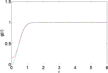
Figure 3: Pair correlation functions for the 2D one-component plasma at $\Gamma=2$ with (red) and without (green) short-range potential correction. When the short-range potential is corrected the exact solution (also plotted) and simulation result overlap.

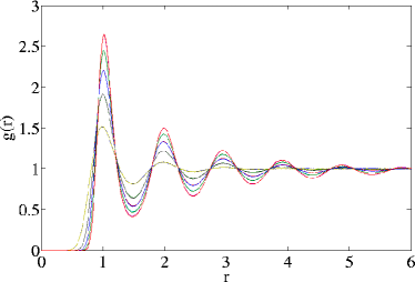
Figure 4: Pair correlation function $g(r)$ for the 2D one-component plasma for $\Gamma$ equal to $20$,$40$,$60$,$80$,$100$. Results plotted for simulations with local update, and with the potential energy computed as a Lekner summation.

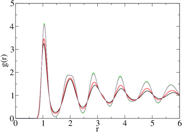
Figure 5: Pair correlation function $g(r)$ for the 2D one-component plasma for $\Gamma=140$. Five curves are shown. The gray curve is for a global continuum method. The green and blue curves that match it were found using the local method with a short-range correction extending about $1/3$ of the total distance across the system from each charge. They are distinguished by either including independent uniform field sampling (green) or not (blue). The two less correlated curves (red and black) are respectively with and without uniform field sampling. They are less correlated than the other three curves because the corrections to the potential extend only half of the distance from each charge compared to the more correlated case.

I have also computed the average energies of the charged particle system using the Lekner summation as a further test of the local method. Of course, global energy calculations at each step defeat the object of the local algorithm, which is most efficient if we are only interested in charge correlations. Anyway, the energies from this work agree temperature for temperature with results obtained by Leeuw and Perram Leeuw2 to their degree of accuracy.

IV.3 Autocorrelation times of charges

In this section and the following, we present various autocorrelation times denoted $\tau$ which are characteristic times of the autocorrelation function

$$A(k)=\frac{\langle O_{i}O_{i+k}\rangle-\langle O_{i}\rangle^{2}}{\langle O_{i}^{2}\rangle-\langle O_{i}\rangle^{2}}$$

where $O_{i}$ for $i=1,\ldots,N$ is a sequence of data obtained from the Monte Carlo simulation and the angled brackets denote a thermal average. These times provide a measure for the rate of relaxation of different observables over the course of the simulation. They depend on the update method, on the nature of the particles and their interaction and on the choice of $O$. We measure these using both a binning procedure Janke ; Sokal and by integrating the autocorrelation function. We find the numbers are consistent with one another, though the former method is preferable because it signals convergence to $\tau$. We present results in this section for two typical observables at various temperatures. After an equilibration process from a hot start, the algorithm is allowed to adjust the maximum step size $\Delta\mathbf{r}$ that each charge can make from its original position so that the acceptance rate for charge moves is $50\%$ . The sampling is performed with this fixed maximum step size. A similar and simultaneous procedure is adopted for the plaquette update step in the local simulation. Because we are concerned with charge observables in this section, we measure autocorrelation times in units of charge move trials; in other words independent transverse field updates are not included in the estimates.

Figure 6 shows a rise in the energy autocorrelation time as $\Gamma$ increases; as the temperature is lowered, energy fluctuations become more improbable so the step size $\Delta\mathbf{r}$ falls to retain the fixed acceptance rate. The autocorrelation time falls coincidently. Over the range $\Gamma=2$ to $\Gamma=80$ there is roughly a tenfold increase in $\tau$ for both the Lekner and local methods. The autocorrelation times are consistently much larger for the local method than for the Lekner method. That the local simulation $\Delta\mathbf{r}$ should be smaller than that for the Lekner simulation is to be expected on the following grounds. In the absence of charges, a single charge has to overcome an energy barrier, on average, to make a move using the local method. This is because it has to move in its own field which relaxes locally to maintain Gauss’ law. This can be seen most easily in the case of a single charge confined to a lattice vertex. If we ignore field circulation changes which only produce fluctuations about the average that we consider here, a step in the position of the charge takes a single link field from $E$ to $E-(q/a)$ where $E=q/4a$ (in 2D) on average; the energy difference is then $q^{2}/4>0$. In contrast, a single charge in a periodic cell in the Lekner simulation has no barrier to overcome to make a move on average. The qualitative observation that the energy barrier for a given step size is higher in the local method than in the global method is true regardless of the number of charges present in the cell.

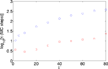
Figure 6: Autocorrelation times for the energy on a logarithmic scale varying with $\Gamma$. The circles are data for the local method, squares for the Lekner simulation.

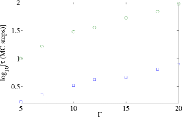
Figure 7: Variation of $\log_{10}(\tau)$ of the structure factor for $\mathbf{k}$ vector $(10,6)$ (close to the first reciprocal lattice vector) with inverse temperature $\Gamma$ in the liquid phase which exhibits short-range correlations. The local simulation (circles) relaxes more slowly than the global simulation method with a Lekner potential.

I have also computed the structure factor for $k$ vector close to the first reciprocal lattice vector for our two different simulation methods. As correlation develops in the sample, a peak forms in the structure factor at reciprocal lattice vectors. The structure factor at these values of $k$ are the slowest to relax so we have concentrated on high temperatures compared to the reported phase transition temperature to ensure good results. Once again, we find that $\tau$ is much larger for the local simulation method than for the global method as can be seen from Figure 7, which uses a logarithmic scale to represent the autocorrelation times.

IV.4 The relative speed of the local algorithms

In previous works, the $O(N)$ scaling of the local method has been pointed out. But, such scaling cannot be of much use if the scaling prefactor or, in other words, the absolute times are prohibitively large even for small systems. In this section, we shall see that in comparison with the Lekner summation simulations, the local method fares very well even when the differing autocorrelation times are included. The autocorrelation time provides a measure for the efficiency with which simulation methods can sample configuration space. Specifically, if a single run gives a sequence of $n$ values of some observable with variance $\sigma_{O_{i}}^{2}$, the variance of the data about the ensemble average for that observable is given by Janke ; Sokal

$$\sigma_{\mbox{\={O}}}^{2}=\sigma_{O_{i}}^{2}\frac{2\tau}{n}.$$ (12)

We use the autocorrelation time of some observable to find the number of sweeps required to bring the variance about the ensemble mean down to some value and hence obtain the absolute simulation times taking into account the differing charge relaxation times. Different observables have different autocorrelation times in general but to make a comparison of absolute speeds in this way we have to choose one. We have chosen $S(\mathbf{k}=\mathbf{G})$, because, as a charge correlation function, it is a quantity that is both interesting and which the local algorithm is particularly suited to computing. Also, the reciprocal lattice vector is likely to give the slowest relaxation of charge observables, so the test will provide something of an upper bound on times. It should be emphasized that the autocorrelation time for sufficiently high temperatures or sufficiently large system sizes, is independent of system size provided it is measured in Monte Carlo sweeps. So, the comparison made in this section does not affect the scaling of the algorithms. This is not the case close to phase transitions, which would require a separate analysis, or for very small system sizes.

I have measured the time taken for both the local and Lekner algorithms to complete a given number of particle moves for two system sizes $N=120$ and $N=1000$. This time depends, of course, on the code, the compiler and the machine that is used so we don’t expect the numbers presented here to demonstrate any more than trends in the absolute and relative speeds and rough estimates for the absolute speed. The Lekner method scales as $O(N^{2})$ but it has the advantage that it is easy to implement and the time taken for a charge move should be smaller than in $O(N)$ molecular dynamics methods for typical system sizes.

The code with local updates has a short-range potential correction routine with a $6\times 6$ plaquette region within which the correction is performed. The simulation cell is a $32\times 32$ mesh. The number of plaquette updates per particle move is maintained at $40$ so that the mobility is close to maximum as we shall see in Section IV.5. The cell size is chosen so that the charge density is one.

The raw speed of the local code before including the correlation in the data is obviously much greater than that of the global code because the overheads are so much smaller when just a few links need to be changed. We also find that the times scale as $N$ for the Lekner code as expected. The time interval for a fixed number of steps in the local code does vary with $N$ only because the number of particles captured by the short-range correction routine increases with $N$. In fact, the short-range correction makes a very significant contribution to the speed: for a cell with $200$ charges, switching off the correction routine halves the time interval. When the number of plaquettes increases holding the number of particles per plaquette constant, the speed of the local update code does not change significantly.

In the previous section, the variation of $\tau$ for $S(\mathbf{k}=\mathbf{G})$ with temperature was given. We have also measured the mean and variance of the structure factor for each temperature from the data. Suppose we want to estimate $S(\mathbf{k}=\mathbf{G})$ to within $1\%$. We obtain the required number of configurations $n$ from equation (12).

$\Gamma$	5.0	7.0	10.0	12.0	15.0	18.0	20.0
$\tau$	1.7	2.25	3.3	4.2	4.6	6.5	7.9
/MC sweeps	10.0	16.4	30.0	35.6	53.2	68.4	94.4
No.MC sweeps for	7.7	11.0	17.8	23.7	27.8	42.8	53.9
$1\%$ s.d./ $10^{3}$	45.6	80.7	162.6	199.4	325.6	446.0	641.9
Simulation time	10.7	15.4	24.9	33.2	38.9	60.0	75.0
120 charges/min	4.9	8.6	17.3	21.2	34.7	47.5	68.3
Simulation time	12.6	18.1	29.2	39.0	45.7	70.5	88.7
1000 charges/hr	3.2	5.7	11.5	14.0	23.0	31.5	45.3

Table 1: Table of speeds of the Lekner and local simulation methods taking into account the fact that their autocorrelation times differ. We used a 1004MHz, AMD Athlon x86 64 bit processor with Linux operating system and suitably optimized gcc compilation. The upper figure in each box is for the Lekner summation Monte Carlo, the lower number for the local method.

Table 1 gives, for seven temperatures, the autocorrelation time of the first reciprocal lattice peak of the structure factor (which has already appeared in Figure 7), the variance in the configuration values about the mean and hence the number of sweeps required to get the error of $S(\mathbf{k}=\mathbf{G})$ to $1\%$ of the mean value. From our measurements of the speed of each piece of code, we estimate the minimum amount of time the global and local simulations should be allowed to run to obtain data of this quality for $N=120$ and $1000$. The effect of including the autocorrelation times is contained in the two lowest rows. The local code remains the faster of the two, for both system sizes and for all temperatures but inclusion of the relaxation times has narrowed the gap considerably. For $\Gamma=20$ and $N=120$ the necessary times are brief (as we would expect at these fairly high temperatures compared to the phase transition) and similar. The scaling of the speeds with the number of charges implies a larger difference for $N=1000$ but the absolute times are becoming inconveniently large.

IV.5 Transverse field relaxation

The unique feature of the local simulation method is the introduction of transverse field degrees of freedom. These degrees of freedom should scale roughly with $N$, the number of charges in the system to preserve the accuracy of results. One might expect that the transverse electric field should be allowed to relax all the way across the system at each charge move, with the result that the algorithm should scale as $O(N^{2})$. In practice, we find that a very low rate of independent plaquette updates $O(1)$ is all that is required per charge move to obtain good sampling at intermediate temperatures $2<\Gamma<140$ and, at higher temperatures, plaquette updates can be switched off altogether. At lower temperatures, we find that one must sample the transverse field at a higher rate per charge move.

In this section, we investigate these properties. To do this, we have measured the autocorrelation time $\tau$ of the background uniform electric field as the rate of plaquette updates is changed. The uniform field does not depend directly on the plaquette circulation; it varies as charges move by the local update method as discussed in Section II, so this quantity provides a measure for the charge relaxation times that is particularly straightforward to investigate compared to relaxation times of charge correlation functions.

Figure 8 shows how $\tau$ varies when the plaquette update rate is varied. The horizontal axis in the figure is

$$\frac{\mbox{Rate of plaquette updates}}{\mbox{Rate of particle updates}}\equiv\alpha.$$

We find that, as $\alpha$ increases from zero for intermediate temperatures, $\tau$ decreases sharply and reaches a vale. Over the temperature range $5\leq\Gamma\leq 140$ that we have investigated, the behavior of $\tau$ is so weakly dependent on temperature that the data almost collapse. A similar behavior is seen in the mobility of charges,(defined here as the gradient taken from the plot of RMS distances of charges from their original positions against simulation time measured in Monte Carlo sweeps). The mobility is close to maximum for a very low rate of plaquette updates: just one update per particle move on average although there are $32\times 32$ plaquettes and roughly one particle for nine plaquettes. We have also looked directly at the autocorrelation times of different modes of the transverse field with the same temperature independence even close to the transition. At higher temperatures $\Gamma<20$, we see a significant change in the behavior of $\tau$ for the uniform field. The same figure 8 shows data for $\Gamma=2$ for which $\tau$ falls below the lower temperature data at $\Gamma=5$ at small $\alpha$. We have also been able to obtain the $\alpha=0$ point for $\Gamma=2$ which is too large at lower temperatures to obtain accurately. This high temperature behavior matches the qualitative result that good averages are obtained at high temperatures $\Gamma\leq 2$ without plaquette updates.

We can understand this behavior qualitatively as follows. We have already pointed out that in the absence of plaquette updates, the electric field is altered by the motion of charges, which leave trails of altered field along their paths. The effect of the trail on each charge is to restore it to its original position. So, at least, at low temperatures, we expect charges to be trapped in their original positions with a correspondingly long autocorrelation time of the uniform field which oscillates with the charges. When the electric field is allowed to relax by changing the circulation around plaquettes, the string is smeared across the system and the restoring force on each charge falls on the average and hence the charges become mobile. There must be some limiting mobility at a fixed temperature. We expect that smearing of the trails can also take place purely by the motion of charges - an effect which is presumably enhanced by spreading charges over more lattice sites. But this smearing of trails by charges is contingent on at least some independent plaquette updates. At high temperatures, charges can overcome the potential barriers around their initial positions so $\tau$ for the uniform field is small.

We would like to understand why the maximum mobility is attained with such a low update rate at intermediate temperatures. We shall see that a simple probability model for the update process exhibits a similar feature. Suppose there are $N$ plaquettes, each one inhabited, on average, by a charge. At each step, the probability of choosing a plaquette is $P_{p}$ and the probability of choosing a charge $P_{c}$. The ratio $P_{p}/P_{c}\equiv\alpha$. So

$$\begin{array}[]{lr}P_{p}=\dfrac{\alpha}{\alpha+1}&P_{c}=\dfrac{1}{\alpha+1}.\end{array}$$

A plaquette is said to be free if a charge on that plaquette can move freely (it does not leave an electric field trail). Otherwise, it is trapped. The number of free plaquettes is $N_{F}$. The following processes are possible

1. Plaquette move frees plaquette: $N_{F}(t_{i-1})+1=N_{F}(t_{i})$

2. Plaquette move traps plaquette: $N_{F}(t_{i-1})-1=N_{F}(t_{i})$

3. Particle move on trapped plaquette: $N_{F}(t_{i-1})=N_{F}(t_{i})$

4. Particle move on free plaquette: $N_{F}(t_{i-1})-1=N_{F}(t_{i})$.

The fourth rule that a charge moving on a free plaquette causes the plaquette to become trapped has its basis in the fact that a moving charge leaves a line of electric field when it moves. The probability distribution function of the number of free plaquettes satisfies a master equation

$$\frac{\partial P(N_{F},t)}{\partial t}=J(N_{F})-J(N_{F}+1,t)$$

where

$$J(N_{F})=\frac{\alpha}{\alpha+1}\frac{N-N_{F}+1}{N}P(N_{F}-1,t)-\frac{N_{F}}{N}P(N_{F},t).$$

We solve for the stationary (time-independent) probability distribution in the usual way Gardiner . Form the summation

$$\sum_{i=0}^{M-1}\left[J(i+1)-J(i)\right]=J(M)-J(0).$$

The boundary conditions on the rates give $J(0)=0$ and hence

$$P(N_{F})=\frac{\alpha}{\alpha+1}\frac{N-N_{F}+1}{N_{F}}P(N_{F}-1).$$

We compute the mean number of free plaquettes $\langle N_{F}\rangle$ as the ratio $\alpha$ is changed. The mean number of free plaquettes is essentially equivalent to the number of free charges and is therefore indicative of the mobility. We find that $\langle N_{F}\rangle$ tends rapidly to a maximum of half of $N$ as $\alpha$ is increased (see Figure 9). Around $10$ plaquette updates per particle move are sufficient to bring $\langle N_{F}\rangle$ within $5\%$ of maximum just as is the case for mobilities in the simulations presented above. Of course, this model is hugely oversimplified. There are many ways in which the simulation updates differ from the processes in this model. For example, the simulation uses a Monte Carlo test to carry out updates, charges are spread over four plaquettes and we have simulated at a particle density of about $1$ particle to $9$ plaquettes (neglecting spreading). Also, a charge can erase a trail by moving along it: a trapped plaquette can be freed up by charge motion. Nevertheless, the model captures the important feature of the changing mobility: if more than one plaquette is freed per particle move, $N_{F}$ increases until limited by the unfreeing operation. We therefore expect the limiting number of free plaquettes to be half of the total.

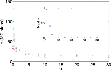
Figure 8: Variation of the integrated autocorrelation time of the uniform background field with plaquette update rate measured in average number of plaquette moves per particle move. Results for four different temperatures are shown: $\Gamma=2$,$5$, $20$,$40$, $60$ and $140$ (circles,stars,crosses,squares,diamonds and triangles respectively). The definition of $\alpha$ is given in the main text. The inset shows the gradient of RMS distance of particles from their original positions varying with $\Gamma$.

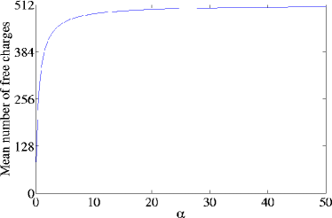
Figure 9: $\langle N_{F}\rangle$ as a function of $\alpha$ showing the rapid approach to $512$ where there are $1024$ plaquettes in total.

We turn now to the behavior at low temperatures around the transition temperature. We find that a high rate of plaquette updates is necessary to achieve the same degree of correlation one finds with the Lekner summation method. For $\Gamma=120$ and $140$, I have obtained pair correlation functions at different values of $\alpha$ in the range $\alpha=2$ to $\alpha=100$. All the $\Gamma=120$ results are identical and match the pair correlation function using the Lekner Monte Carlo method. The $\Gamma=140$ results differ, with convergence onto the Lekner result for around $\alpha=40$. I have not investigated this further but it is worth pointing out that the slower convergence to the correct result as $\alpha$ is varied happens close to the transition temperature where one would expect charge relaxation times to be longer than in the fluid phase. There is no remarkable behavior close to the transition temperature in the uniform field relaxation time nor in the transverse field relaxation time. For practical purposes at such low temperatures, the unbiased plaquettes updates are inefficient and it may be sensible to use a worm update to sample transverse degrees of freedom Review which involves the creation of a pair of equal and opposite charges, at intervals during the simulation, which wander around the simulation cell and eventually annihilate.

We conclude this section with three observations. The first concerns the relationship between the mobility (defined above) and the autocorrelation time of the uniform field $\tau$. We have found that as $\tau$ falls, the mobility rises. For low $\alpha$, this is consistent with the picture of charges trapped by their electric field trails. However, the mobility is also temperature dependent as can be seen in the inset plot of Figure 8. At low temperatures, the mobility is small although the uniform field may relax quickly. So, $\tau$ appears to be independent of the mobility. Notice however, that the greatest temperature change in the mobility and in $\tau$ occurs for $\Gamma<20$ whereas for $\Gamma>20$ both are only weakly temperature dependent, so they are more (anti)correlated for low $\alpha$.

The second observation is that the curve of uniform field $\tau(\alpha)$ depends on the number of charges $N$ and the number of plaquettes $P$ only in the ratio $P/N$. If the number of plaquettes increases, holding the number of charges constant, the autocorrelation time increases because the fraction of plaquettes updated per particle move drops. When $N$ increases in proportion to $P$, the data collapses onto the curve in Figure 8.

Finally, the results described in this section lead to the conclusion that if charges can overcome the impetus to retrace the electric field trails they produce (which will typically be at high temperatures), then thermal averages will be electrostatic averages even in the absence of independent plaquette updates. After all, the Metropolis algorithm guarantees that averages from computer generated configurations will converge to thermal averages (which in this case are electrostatic averages) provided that all of configuration space can be sampled in principle. In practice, reasonable mobilities can be achieved at high temperature with no plaquette updates. At lower temperatures, a few plaquette updates are required to overcome bottlenecks while electric field trails are altered by charge motion and charges can cooperate in freeing other charges provided they are dense enough that charge clouds overlap to some extent.

Although charge dynamics depends on electric field circulation and vice versa, the factorization of transverse and longitudinal energies ensures that these contributions to the fields are importance sampled independently and simultaneously. Relaxation of transverse fields across the periodic sample at each charge step is unnecessary because we are interested in averages over many configurations. It is sufficient that relaxation can occur over a number of charge steps. At the end of the simulation with no information discarded, one can ’project’ onto each link transverse field to find it has been sampled adequately. Each transverse field is a harmonic oscillator for which good thermal averages are easily obtained and even with a separate transverse degree of freedom of each link, most of the work goes into sampling charge configurations.

If this conclusion is correct, one would expect that the charge dynamics introduced in Section III.1 in the presence of thermal noise should be sufficient to recover electrostatic averages. Unfortunately, the evolution of the electric field configuration is not a Markov process so further analysis is difficult.

V Summary and conclusions

We have made a study of a local Monte Carlo method developed by Rottler and Maggs RottlerMaggs for simulating systems of charged particles. The unrefined method is limited in the accuracy it can achieve, because the electric field is discretized onto a lattice. One must remove self-energy contributions due to charge spreading and correct the short-range interaction. All these can be done locally, so the scaling of the method is $O(N)$ where $N$ is the number of charges.

1. Simulations of the 2D one-component plasma have been carried out in one of the first applications of the local off-lattice Monte Carlo method. With a short-range interaction correction extending a distance of about a tenth of the length $L$ of each simulation cell from each charge, excellent results are obtained for the pair correlation function for $\Gamma\leq 100$. By making the method less local results can be obtained to lower temperatures. For example, with short-range correction a distance of $L/5$ from each charge, good results can be obtained at least down to the transition temperature $\Gamma\sim 140$.

2. Although there is a non-vanishing uniform electric field during our local simulation which is a consequence of the charge move update, we find that this produces no significant deviation from results obtained from an Ewald potential for which the dipole term is zero. It is not certain from this study whether this result will generalize to all systems containing many mobile charges but I suspect that the electric field will indeed average out because charge winding, which gives an electric field that cannot be inferred from the particle positions, is always important.

3. In order to obtain accurate results at low temperatures ($\Gamma\sim 140$), a much larger rate of plaquette updates is necessary than at lower temperatures. This is correlated with the fluid-crystal transition. Plaquette updates are completed much more quickly than charge moves so this effect does not substantially alter the speed though of course charge autocorrelation times are larger at lower temperatures so simulations should be longer anyway. One might introduce a worm update to sample the transverse electric field more efficiently at low temperatures though it would seem to be unnecessary otherwise, at least for the 2D OCP.

4. The charge autocorrelation times for the local method are much larger than for global methods. This is because there is, on average, a larger energy barrier to charge motion when Gauss’ law is maintained locally.

5. The autocorrelation times should be included in calculations of the effective speed. When this is done for system sizes that are typically simulated, we find that the gap between the local method and the $O(N^{2})$ global method is considerably narrowed compared to the raw speeds, but that the local method remains significantly faster and the gap widens as the number of charges increases. We have not studied molecular dynamics methods which in some cases have $O(N)$ scaling. Preliminary results by Pasichnyk and Dünweg Dunweg suggest that molecular dynamics adapted from the local Monte Carlo we have discussed here is a promising alternative to the P³M method. But, we expect Monte Carlo to have the advantage of relative ease of implementation and smaller scaling prefactor. The most significant contributions to the prefactor are charge assignment, local field updates and especially corrections to the lattice potential. Except at low temperatures, plaquette updates are not a significant factor in the speed.

6. We also looked at the question of how the introduction of extra degrees of freedom can result in a faster method when naively we would expect the transverse degrees of freedom should be allowed to relax across the simulation cell for each charge move. Charge mobility for intermediate temperatures is seen to increase sharply as the rate of plaquette updates is increased from zero. We have provided a simple model that, from a reasonable premise, reproduces this qualitative behavior. For high temperatures $\Gamma\leq 2$, the charge mobility is large even when independent plaquette moves are switched off. The fact that plaquette updates can be switched off at high temperatures strongly suggests that importance sampling of the simple transverse degrees of freedom can be accomplished entirely by charge moves, provided they are sufficiently mobile.

7. We have introduced a continuum version of the charge move electric field update which allows us to see more rigorously that charge moves alter the transverse electric field. Following from the observation in the previous point, an interesting problem is to carry out the average over electric fields using this dynamics alone and hence recover electrostatic averages.

8. In an appendix, we have showed that a thermal average over Maxwell electrodynamics for a system of charges gives the same charge correlation functions one would obtain from electrostatics alone. As is well-known, the magnetic field has no effect on correlation functions. Also, the transverse part of the electric field averages out as in the original discussion by Maggs and Rossetto.

Appendix A Approximation to the Ewald potential in two dimensions

In this section, we find a good approximation to the Ewald potential in two dimensions for small charge separations. Consider 2 charges $q$ in a rectangular periodic cell with side lengths $L_{x}$ and $L_{y}$. The whole system is charge neutral because a neutralizing charge is smeared uniformly over the cell. Leeuw and Perram Leeuw have found that the total energy can be expressed as

$$2\pi U=\frac{q^{2}}{4}\sum_{\mathbf{n}}\sum_{i,j=1}^{2}\star E_{1}\left(\alpha^{2}(\mathbf{r}_{ij}+\mathbf{n})^{2}\right)\\ +\frac{q^{2}}{2\pi A}\sum_{\mathbf{k}\neq 0}\frac{\exp(-\pi^{2}\mathbf{k}^{2}/\alpha^{2})}{\mathbf{k}^{2}}\left[1-\cos(2\pi\mathbf{k}\cdot\mathbf{r}_{12})\right]\\ -\frac{q^{2}}{2}\left(\gamma+\ln\alpha^{2}A\right)-\frac{q^{2}\pi}{\alpha^{2}A}$$ (13)

where the $\star$ means that we should not include the charge self energy in the summation over $\mathbf{n}=(n_{x},n_{y})$ and $n_{i}$ are integers. The area of the system is $A=L_{x}L_{y}$ and $\gamma$ is Euler’s constant. The energy does not depend on constant $\alpha$ but the rate of convergence of the summations does. This is the energy of the interaction between the charges and their periodic images, interaction of the charges with the background charge and the self-energy of the background. We would like to subtract off the background contributions. The interaction between two charges without images is just $(q^{2}/2\pi)\ln(1/r)$. So we compute

$$U_{\mbox{\small bkg}}=\lim_{r\rightarrow 0}{U+\dfrac{q^{2}}{2\pi}\ln r}$$

because the interaction of the charges with their images are guaranteed to vanish in the limit. Hence the interaction between the charges is given by $U_{int}=U-U_{bkg}$. We find

$$2\pi U_{int}=\frac{q^{2}}{2}E_{1}(\alpha^{2}\mathbf{r}^{2})\\ +\frac{q^{2}}{2\pi A}\sum_{\mathbf{k}\neq 0}\frac{\exp(-\pi^{2}\mathbf{k}^{2}/\alpha^{2})}{\mathbf{k}^{2}}\left[-1+\cos(2\pi\mathbf{k}\cdot\mathbf{r})\right]\\ -\frac{q^{2}}{2}(\gamma+\ln\alpha^{2})$$ (14)

where the distance between the charges is denoted $r$. We approximate the exponential integral for small $r$

$$E_{1}(\alpha^{2}r^{2})=-\gamma-2\ln\alpha r+\alpha^{2}r^{2}+\dots$$

We now turn to the $k$ space summation which, for small $r$ is

$$-\frac{q^{2}}{4\pi A}\sum_{\mathbf{k}\neq 0}\frac{\exp(-\pi^{2}\mathbf{k}^{2}/\alpha^{2})}{\mathbf{k}^{2}}\left(2\pi\mathbf{k}\cdot\mathbf{r}\right)^{2}-\frac{q^{2}}{2}(\gamma+\ln\alpha^{2}).$$

The cross-terms in $\mathbf{k}\cdot\mathbf{r}$ vanish because the summation is over positive and negative integers. We can also remove a factor of $r^{2}$ because the terms in the summation are identical. Then we use the identity

$$\sum_{\mathbf{k}}\exp{-\pi^{2}\mathbf{k}^{2}/\alpha^{2}}=\frac{\alpha^{2}A}{\pi}\sum_{\mathbf{n}}\exp{-\alpha^{2}A\mathbf{n}^{2}}$$

and approximate the exponential for large $A$, retaining the terms to order $A$. We find that the short range correction energy $U_{SRC}$, which approximates $U_{int}$, is

$$U_{SRC}=-\dfrac{q^{2}}{2\pi}\ln r+\dfrac{q^{2}r^{2}}{4A}$$ (15)

the terms depending on $\alpha$ cancel. The calculation in three dimensions is given in an appendix to Fraser .

We compare this result with the Ewald potential. The figure (10) shows how the approximation to the short range correction given by equation (15) differs from the Lekner interaction $V$ from equation (3) as the charge separation increases. The measure we use is

$$\frac{\Delta V(x)-\Delta U_{SRC}(x)}{\Delta V(x)}$$

where $\Delta U_{SRC}(x)$ and $\Delta V(x)$ are energy differences as a charge steps outwards by half a lattice spacing from separation $x$. The error is within $1\%$ for charge separations of $1/5$ of the cell width $L_{x}$ and for the highest accuracy low temperature simulations we performed, up to $2\%$.

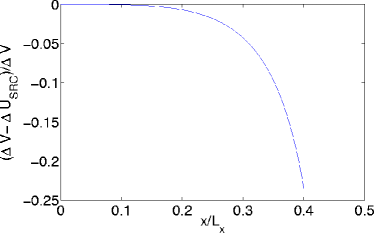
Figure 10: Plot of the normalized error between energy differences calculated using the Lekner potential and the short range interaction potential (15). We have used parameters appropriate to the simulations we have performed, with $32\times 32$ square plaquettes covering the cell and lattice spacing $a=0.342$. The energy differences are for charge steps in the $x$ direction through a distance of one-half of the lattice spacing. $L_{x}$ is the width of the periodic cell in the $x$ direction.

Appendix B Electrostatics from thermal electrodynamics

In this part we wish to demonstrate that the argument Maggs and Rottler have made for their rather unphysical energy function holds also for full Maxwell electrodynamics. That is to say that even though the charges do not influence one another by instantaneous action at a distance, they nevertheless generate thermodynamic averages as though they do. This result has already been found by Alastuey and Appel Alastuey but I believe it would be useful to present the argument in this context. The main difficulty is in finding an energy functional that includes the constraints that depend on the static configuration of charged particles.

The charges are not subject to an external field but are influenced by other charges in our hypothetical box in a heat bath. Since the fields are dynamical quantities we must include them in our discussion. So, the Lagrangian for a system of $N$ relativistic charges $q_{i}$ for $i=1,2,\ldots,N$ interacting electrodynamically is

$$L=\sum_{i=1}^{N}-m_{0i}\sqrt{1-\mathbf{v}_{i}^{2}}+\int d^{3}\mathbf{r}\left(-\frac{1}{4}F_{\mu\nu}F^{\mu\nu}+J_{\mu}A^{\mu}\right)$$

where $\{\mathbf{v}_{i}\}$ are the particle velocities and $\{m_{0i}\}$ their rest masses. $F_{\mu\nu}\equiv\partial_{\mu}A_{\nu}-\partial_{\nu}A_{\mu}$ is the electromagnetic field tensor defined in terms of $4$-vector potential $A_{\mu}$. The $4$-vector current has components $J^{0}$ which is the charge density and spatial components in $3$-vector $\mathbf{J}=\sum_{i}\delta(\mathbf{r}-\mathbf{r}_{i})q_{i}\mathbf{v}_{i}$. We have taken $c=1$.

The form of the Lagrangian ensures that the homogeneous Maxwell equations are obeyed

$$\partial_{\mu}F_{\nu\sigma}+\partial_{\sigma}F_{\mu\nu}+\partial_{\nu}F_{\sigma\mu}=0\left\{\begin{array}[]{r}\mathbf{\nabla}\cdot\mathbf{B}=0\\ \mathbf{\nabla}\times\mathbf{E}=-\frac{\partial\mathbf{B}}{\partial t}\end{array}\right.$$

The first step in getting a Hamiltonian is to find the conjugate momenta from the Lagrangian. For the charges, the momenta are

$$\mathbf{p}_{i}=\frac{\partial L}{\partial\mathbf{v}_{i}}=\frac{m_{0i}\mathbf{v}_{i}}{\sqrt{1-\mathbf{v}_{i}^{2}}}+q_{i}\mathbf{A}_{i}$$

where $\mathbf{A}_{i}=\mathbf{A}(\mathbf{r}_{i})$ and for the fields

$$\Pi^{\mu}=\frac{\partial\mathcal{L}}{\partial_{0}\mathbf{A}_{\mu}}=-F_{0\mu}$$

where $\mathcal{L}$ is the Lagrangian density. We notice that $\Pi^{0}$ vanishes because $F^{\mu\nu}$ is antisymmetric. The equations of motion are

$$\partial_{\mu}F^{\mu\nu}+J^{\nu}=0.$$

If we go straight ahead and find the Hamiltonian for the fields and the interaction term

$$H_{F}=\int d^{3}\mathbf{r}\,\mathbf{\Pi}\cdot\dot{\mathbf{A}}-\int d^{3}\mathbf{r}\left(-\frac{1}{4}F_{\mu\nu}F_{\mu\nu}+J_{\mu}A^{\mu}\right)$$

we get

$$H_{F}=\int d^{3}\mathbf{r}\,\left(\frac{1}{2}\left(\mathbf{B}^{2}+\mathbf{E}^{2}\right)-\mathbf{J}\cdot\mathbf{A}\right)$$

in terms of the electric and magnetic fields having used an equation of motion after partial integration to write

$$\mathbf{\Pi}\cdot\dot{\mathbf{A}}=F_{0i}F_{0i}+A_{0}J^{0}.$$

In this form, we cannot perform an average over the electric field because it is constrained by Gauss’ law

$$\mathbf{\nabla}\cdot\mathbf{E}=J^{0}$$

which is formally an equation of motion although it is a static constraint on the field. We shall now render the Hamiltonian in a form that brings out the important constraints. To do this, we first notice that the electric field can be split into rotational and irrotational parts, exactly as we did in the introduction. Using the same notation as before

$$\mathbf{E}=\mathbf{E}_{\|}+\mathbf{E}_{\bot}.$$

We also recall that the Lagrangian for electrodynamics is gauge invariant. We can fix the gauge to reduce the arbitrariness in $\mathbf{A}$. For our purposes it is useful to choose the so-called Coulomb gauge $\mathbf{\nabla}\cdot\mathbf{A}=0$. This can always be done. The reason for choosing this gauge is that the splitting of the electric field into transverse and longitudinal parts is mirrored in the vector potential in the following nice way

$$\begin{array}[]{cc}\mathbf{E}_{\|}=-\mathbf{\nabla}A^{0}&\mathbf{E}_{\bot}=-\dfrac{\partial\mathbf{A}}{\partial t}.\end{array}$$

We see that Gauss’ law in terms of $A_{0}$ is Poisson’s equation which has the solution

$$A^{0}(\mathbf{r},t)=\int d^{3}\mathbf{r}^{\prime}\ \frac{J^{0}(\mathbf{r}^{\prime},t)}{4\pi|\mathbf{r}-\mathbf{r}^{\prime}|}$$

which is the instantaneous Coulomb interaction. The transverse field is independent of the Gauss’ law constraint. It is also significant that, as before, the electric field energy splits into independent transverse and longitudinal energies

$$\frac{1}{2}\int d^{3}\mathbf{r}\ \mathbf{E}^{2}=\frac{1}{2}\int d^{3}\mathbf{r}\ \mathbf{E}_{\bot}^{2}+\frac{1}{2}\int d^{3}\mathbf{r}d^{3}\mathbf{r}^{\prime}\ \frac{J^{0}(\mathbf{r})J^{0}(\mathbf{r}^{\prime})}{4\pi|\mathbf{r}-\mathbf{r}^{\prime}|}.$$

Henceforth we denote the longitudinal field energy by $V$. Now that we have put the longitudinal dependence into $A^{0}$ we would like to have a momentum variable that is independent of $A^{0}$. We choose $\mathbf{\Pi}_{\bot}=\mathbf{\Pi}-\mathbf{\nabla}A^{0}$ which must satisfy the constraint $\mathbf{\nabla}\cdot\mathbf{\Pi}_{\bot}=0$ that follows directly from the gauge constraint. We must get the Hamiltonian from this new momentum. For the field quantities

$$H_{F}=\left(\int d^{3}\mathbf{r}\ \mathbf{\Pi}_{\bot}\cdot\dot{\mathbf{A}}\right)-L_{F},$$

where $L_{F}$ is the Lagrangian excluding the field-independent parts, so that the complete energy function (including the free particle and interaction terms) is

$$H=\sum_{i}\sqrt{\left(\mathbf{p}_{i}-q_{i}\mathbf{A}_{i}\right)^{2}+m_{0i}^{2}}\\ +\int d^{3}\mathbf{r}\left[\frac{1}{2}\mathbf{\Pi}_{\bot}^{2}+\frac{1}{2}(\mathbf{\nabla}\times\mathbf{A})^{2}+V\right].$$

The partition function in the canonical ensemble with inverse temperature $\beta$ is

$$Z(\beta)=\int\prod_{i}d^{3}\mathbf{p}_{i}\int\prod_{i}d^{3}\mathbf{r}_{i}\int\mathcal{D}\mathbf{\Pi}_{\bot}\delta(\mathbf{\nabla}\cdot\mathbf{\Pi}_{\bot})\\ \times\int\mathcal{D}\mathbf{A}\delta(\mathbf{\nabla}\cdot\mathbf{A})\exp(-\beta H)$$

and the limits of the particle momentum integrations are infinite. The field momentum integration factorizes from the rest. Then we make the change of variables $\mathbf{P}_{i}=\mathbf{p}_{i}-q_{i}\mathbf{A}_{i}$ for each particle. The Jacobian for this transformation is unity because the vector potential does not depend on the momenta. So, the integral over the vector potential also factorizes and we are left with

$$Z(\beta)=Z(\beta)_{\mathbf{P}}Z(\beta)_{\mathbf{\Pi}}Z(\beta)_{\mathbf{A}}\int\prod_{i}d^{3}\mathbf{r}_{i}\exp(-\beta V)$$

which, up to a configuration independent factor is the electrostatic partition function. This is essentially a generalized version of the well-known Bohr-van Leeuwen theorem (see, for example vanvleck ).

References

- (1) A. C. Maggs and V. Rossetto, Phys. Rev. Lett. , 88, 196402 (2002).
- (2) J. Rottler and A. C. Maggs,J. Chem. Phys. , 120, 3119 (2004).
- (3) Metropolis, A. W. Rosenbluth and M. N. Rosenbluth, A. H. Teller and E. Teller, J. Chem. Phys. 21, 1087 (1953).
- (4) J. W. Perram and S. W. de Leeuw, Physica, 103A, 237 (1981).
- (5) L. M. Fraser et al. , Phys. Rev. B, 53, 1814 (1996).
- (6) J. Lekner, Physica, A157, 826 (1989).
- (7) J. Lekner, Physica, A176, 485 (1991).
- (8) N. Grønbech-Jensen, Int. J. Mod. Phys. , C7, 873 (1996).
- (9) M. Deserno and C. Holm, J. Chem. Phys. , 109, 7678 (1998).
- (10) R. W. Hockney and J. W. Eastwood, Computer simulation using particles , McGraw-Hill Inc. (1981).
- (11) L. Levrel and A. C. Maggs, Phys. Rev. E, 72, 016715 (2005).
- (12) A. C. Maggs, J. Chem. Phys. , 120, 3108 (2004).
- (13) L. Levrel, F. Alet, J. Rottler, A. C. Maggs, Pramana, 64, 1001 (2005).
- (14) A.Duncan, R. D. Sedgewick, R. D. Coalson, Phys. Rev. E, 71, 046702 (2005).
- (15) J. Rottler and A. C. Maggs,Phys. Rev. Lett. , 93, 170201 (2004).
- (16) I. Pasichnyk and Dünweg, J. Phys. : condensed matter, 16, S3999 (2004).
- (17) A. C. Maggs, Phys. Rev. E, 72, 040201(R) (2005).
- (18) J. Ginibre, J. Math. Phys. , 6, 440 (1965).
- (19) W. Janke in Proceedings of the Euro Winter School Quantum Simulations of Complex Many-Body Systems: From Theory to Algorithms,Ed. J. Grotendorst, D. Marx and A. Muramatsu, (2002).
- (20) A. D. Sokal in Functional Integration:Basics and Applications (1996 Cargèse summer school ),Ed. DeWitt-Morette, C. , Cartier, P. and Folacci, A. , Plenum, New York, (1997).
- (21) C. W. Gardiner, Handbook of stochastic methods. 3rd edition ,Springer (2004).
- (22) S. W. de Leeuw, J. W. Perram and E. R Smith, Proc. Roy. Soc. , A373, 27 (1980).
- (23) A. Alastuey and W. Appel, Physica A 276, 508 (2000).
- (24) J. H. van Vleck, Rev. Mod. Phys. , 50, 181 (1978).