Large $|V_{ub}|$: A challenge for
the Minimal Flavour Violating MSSM

Abstract:

Under the assumption of Minimal Flavour Violation (MFV), the Unitarity Triangle (UT) can be determined by using only angle measurements and tree-level observables. In this respect, the most accurate quantities today available are $\sin 2\beta_{\psi K_{S}}$, $|V_{cb}|$ and $|V_{ub}|$. Among the latter, $|V_{ub}|$ is at present the quantity suffering from largest systematic uncertainties, given the discrepancy between the inclusive and the exclusive determinations.

We show with a numerical fit how sensitively the MFV-UT determination depends on the choice of $|V_{ub}|$. In addition, we focus on the implications of the inclusive value for $|V_{ub}|$, which favors two non-SM like solutions in the $\overline{\rho}-\overline{\eta}$ plane. We study in detail the possibility of reproducing such solutions within the MFV MSSM. Our findings indicate that the case for the MFV MSSM is in this respect quite problematic, unless the non-perturbative parameters $\xi$ and $B_{K}$ are significantly different from those obtained by lattice methods. As a byproduct, we point out that scenarios with 200 GeV $\lesssim M_{A}\lesssim$ 500 GeV and $\tan\beta\simeq 50$ that predict a significant suppression for $\Delta M_{s}$ in correlation with an enhancement for BR$(B_{s}\to\mu^{+}\mu^{-})$ have to be fine-tuned in order not to violate the new combined bound on the latter decay mode from the CDF and DØ collaborations. Relatively large correlated effects can however still occur for negative values of $\mu$ and large values for $M_{A}\gtrsim 500$ GeV, increasing with increasing $\tan\beta\gtrsim 30$.

1 Introduction

Most of the calculable models of low-energy New Physics (NP) available at present tend to be invasive in the sector of flavour violation and to destroy the very specific pattern of flavour changing neutral current (FCNC) effects predicted by the SM. In the example of SUSY, this happens because of its soft sector. In fact, in absence of compelling symmetries restricting the form of the soft terms, the latter must be parameterized most generally. However, when calculating SUSY contributions to flavour observables with such generic soft terms, it is hard to hide simultaneously all their effects behind the already small SM predictions, which agree rather well with the experimental data. The soft terms parameter space that turns out to survive FCNC constraints looks then very fine tuned and this raises the SUSY flavour problem.

A different, phenomenologically coherent approach, is to assume – on the basis of the success of the SM description of FCNC processes – that the flavour sector of any NP model maintains a natural mechanism of “near-flavour-conservation” [1]. The latter would then allow small effects in exact analogy with what happens for the SM.

This idea has been first elucidated as a meaningful requirement for models of NP at the EW scale by the authors of Refs. [2, 1]. It has then been formalized in [3] as a consistent effective field theory framework, called Minimal Flavour Violation (MFV). In this framework, the SM mechanism of near-flavour-conservation is extended to NP by means of the SM Yukawa couplings. Since the latter are in the SM the only sources of flavour breaking, in MFV they play the role of fundamental “building blocks” of flavour violation and every new source of flavour violation, entering the NP Lagrangian, becomes function of them.

This approach is more general than the so-called constrained MFV (CMFV) [4, 5, 6], in which one also imposes the same operator structure as in the SM.

Recently, the MFV framework of [3] has been applied to the MSSM at low $\tan\beta$, in a detailed numerical study of meson mixings [7]. Thereby, the phenomenological differences between MFV and CMFV have been spelled out. It has also been shown how the implementation of the MFV limit makes SUSY contributions to meson mixings naturally small, even for a SUSY scale of a few hundreds GeV.

If NP is of MFV nature – as the lesson of $B$-factories seems to hint – the findings of Ref. [7] indicate that the search for NP effects in flavour observables is more challenging, but not less important, since MFV models become more predictive. In MFV, the focus is on small, but in many cases visible effects. With increased precision of theoretical methods and the amount of data soon available from the LHCb and later, hopefully, from the Super-B [9], one will have such a level of cross-check among different channels that NP effects of even MFV nature should become visible.

An important test of overall consistency among different flavour processes is certainly the global fit to the CKM matrix, which assumes the SM in all observables. However, it is also important to consider fits where one restricts to specific classes of observables (in particular, suitable ratios thereof) that, when assuming a given NP framework besides the SM, are affected in a controlled way or are not affected at all. A first example of this is precisely CMFV [4, 5, 6], that has been analyzed in detail by the UTfit collaboration [10].

However, as first pointed out in [7], the UT analysis suggested by [4] does not account for the most general framework of MFV. Ref. [7] showed in fact that the definition [3] of MFV does not preclude the ratio $\Delta M_{d}/\Delta M_{s}$ – included in the CMFV UT analyses – to be different from the SM value, and therefore, that it should not be included in MFV UT fits.

As a first aim of this paper, we carry out a MFV fit to the UT. When assuming MFV, the only quantities allowed to enter the fit are angle determinations and measurements of tree-level processes. Concerning the former, we restrict to $\sin 2\beta$ as measured from $B\to\psi K_{S}$, while we do not include $\alpha$ and $\gamma$, for reasons to be explained below. As for tree-level processes, we instead restrict to the semileptonic $B$ decays allowing to access $|V_{ub}|$ and $|V_{cb}|$. In particular, while the value of $|V_{cb}|$ is quite well established, the same cannot yet be said about $|V_{ub}|$, whose inclusive and exclusive determinations are in some disagreement with each other, possibly signaling the presence of an underestimated systematic error in either of the two determinations.

It was noted in ref. [11] that, if one uses the inclusive value for $|V_{ub}|$ in a global UT analysis and parameterizes the presence of NP in a model independent way [12], the fit adjusts the tension between $\sin 2\beta$ and the ‘too high’ value for $|V_{ub}|$ by introducing a small negative new phase $\phi_{B_{d}}=-2.9^{\circ}\pm 2.0^{\circ}$ in the $B_{d}$-mixing (see also [6, 13]).

In the present work, we adopt a somehow complementary point of view, since we focus on MFV. The definition of MFV [3] precludes the existence of new CP violating phases beyond the CKM one. In this framework, we discuss the impact of both the exclusive and the inclusive averages for $|V_{ub}|$ on the UT determination. We show in particular how the inclusive $|V_{ub}|$ favors two non-SM like solutions in the $\overline{\rho}-\overline{\eta}$ plane.

Pursuing the possibility that the inclusive $|V_{ub}|$ determination be the correct one, the next question is whether one can find a MFV extension of the SM able to produce either of the two non-SM solutions mentioned above. In particular, one can consider the shifts in the value of the side $R_{t}$ implied by the two solutions. Since $R_{t}$ is (in the SM) related to the ratio $\Delta M_{d}/\Delta M_{s}$ between the $B_{d}$- and the $B_{s}$-system oscillation frequencies, one can translate the above shifts into required values for the NP contributions to the ratio itself. We consider the explicit example of the MFV MSSM. Our findings indicate that the model is able to produce the required amount of corrections only in certain fine-tuned regions of the parameter space. This conclusion holds, barring a substantial shift (above 2 standard deviations) in the present central values for the low-energy parameters $\xi$ and $B_{K}$.

2 MFV fit of the UT

We now turn to our first task, i.e. the determination of the UT when MFV is assumed. In particular we will focus on the UT side $R_{t}$, which will be the relevant quantity for our subsequent analysis. We have today a whole host of observables, which bear dependence on certain combinations of the CKM matrix entries. Hence the determination of the UT apex $(\overline{\rho},\overline{\eta})$ – and all related quantities – follows from a global fit [14, 10], which can include all or a subset of such observables.

We consider three fits of the UT, namely

• a SM fit, including all the ‘classical’ constraints,

• a MFV fit I, including only tree-level observables and $\sin 2\beta_{\psi K_{S}}$,

• a MFV fit II, analogous to the MFV fit I, but keeping only the inclusive averages for both $|V_{ub}|$ and $|V_{cb}|$.

Concerning the full SM fit, it can be performed by combining all the available experimental information (see [14, 10]) and assuming the SM. The state-of-the-art results for the SM determination of $R_{t}$ from the CKMfitter and UTfit collaborations (95% CL) read

$$\mbox{CKMfitter: }(R_{t})_{\rm SM}=0.868^{+0.118}_{-0.049}~{},~{}~{}~{}\mbox{UTfit: }(R_{t})_{\rm SM}=0.906\pm 0.062~{},$$ (1)

in very good agreement with each other. We have performed our SM global fit, using the CKMfitter package [14, 15], a publicly available FORTRAN framework allowing CKM analyses in various statistical approaches, e.g. the frequentist one, used in the present work. We took advantage of the CKMfitter package also for the other fits performed in the present work. It would be interesting to perform an analogous analysis using the UTfit code, which is however not yet publicly available. The input parameters and constraints used in our global fit is listed in Tables 1 and 2. For $R_{t}$ we find (95% CL)

$$(R_{t})_{\rm SM}=0.892^{+0.112}_{-0.068}~{},$$ (2)

in good agreement with the findings in eq. (1). Eq. (2) will be taken as reference figure in our subsequent analysis.

Parameter	Value	Parameter	Value
$\overline{m}_{c}(m_{c})$	$(1.24\pm 0.037\pm 0.095)$ GeV	$G_{F}$	$1.16639\times 10^{-5}$ GeV-2
$\overline{m}_{t}(m_{t})$	$(162.3\pm 2.2)$ GeV	$f_{K}$	$(159.8\pm 1.5)$ MeV
$m_{K^{+}}$	$(493.677\pm 0.016)$ MeV	$B_{K}$	$0.79\pm 0.04\pm 0.09$
$\Delta m_{K}$	$(3.4833\pm 0.0066)\times 10^{-12}$ MeV	$\alpha_{s}(m_{Z}^{2})$	$0.1176\pm 0.0020_{\rm unif}$
$m_{B_{d}}$	$(5.2794\pm 0.0005)$ GeV	$f_{B_{d}}$	$(0.191\pm 0.027)$ GeV
$m_{B_{s}}$	$(5.3696\pm 0.0024)$ GeV	$B_{d}$	$1.37\pm 0.14$
$m_{W}$	$(80.423\pm 0.039)$ GeV	$\xi$	$1.23\pm 0.06$

Table 1: Input parameters used in our fits. Values are taken from the CKMfitter input table updated to summer 2006 [14], with the exception of $\xi$, for which we take the average performed in [16]. Unless otherwise stated, the first error is Gaussian, the second (where applicable) is uniform.

Turning to the MFV fits, the constraints used are collected in Table 2 and the corresponding results are displayed in Figs. 1-2. Some comments are in order on the choices of $|V_{ub}|$. Concerning the inclusive value, we mention that we tried alternatively all the averages reported in Ref. [17]. The latter are obtained by analyzing the inclusive data through use of three alternative theory prescriptions, namely BLNP [18, 19, 20, 21, 22], chosen in our final fits, and

$$\begin{array}[]{ll}|V_{ub}|^{\rm(incl)}=(44.6\pm 2.0\pm 2.0)\cdot 10^{-4}~{},&\mbox{ HFAG average using DGE \cite[cite]{[\@@bibref{}{DGE}{}{}]}}~{},\\[5.69046pt] |V_{ub}|^{\rm(incl)}=(50.2\pm 2.6\pm 3.7)\cdot 10^{-4}~{},&\mbox{ HFAG average using BLL \cite[cite]{[\@@bibref{}{BLL}{}{}]}}~{}.\end{array}$$ (5)

The choice of the BLNP average is, for our purposes, the most conservative. In fact, in the MFV fit II, it leads to two $R_{t}$ solutions which are closer to the SM one (eq. (2)) than in the cases where one uses either of the two other averages in eq. (5).

Concerning instead $|V_{ub}|^{\rm(excl)}$, other determinations are provided e.g. by Refs. [25] and [26], also quoted in [17]. All of them are consistent with each other and we took the result of [27] for definiteness.

Constraint	Value	Ref.	SM fit	MFV fit I	MFV fit II
$|V_{ud}|$	$0.9738\pm 0.0003$	[14]	✓
$|V_{us}|$	$0.2257\pm 0.0021$	[28]	✓
$\alpha$	$(94\pm 8)^{\circ}$	[10]	✓
$\gamma$	$(83\pm 19)^{\circ}$	[10]	✓
$\Delta M_{d}$	$(0.507\pm 0.004)$/ps	[17]	✓
$\Delta M_{s}$	$(17.77\pm 0.12)$/ps	[29]	✓
$|\epsilon_{K}|$	$(2.221\pm 0.008)\times 10^{-3}$	[14]	✓
$\sin 2\beta$	$0.675\pm 0.026$	[17]	✓	✓	✓
$|V_{cb}|^{\rm(incl)}$	$(41.7\pm 0.7)\cdot 10^{-3}$	[28]	✓	✓	✓
$|V_{cb}|^{\rm(excl)}$	$(39.2\pm 0.7\pm 1.4)\cdot 10^{-3}$	[17]	✓	✓
$|V_{ub}|^{\rm(incl)}$	$(45.2\pm 1.9\pm 2.7)\cdot 10^{-4}$	[17]	✓	✓	✓
$|V_{ub}|^{\rm(excl)}$	$(35.5\pm 2.5\pm 5.0)\cdot 10^{-4}$	[27]	✓	✓

Table 2: Constraints used in the various fits. The first error is Gaussian, the second (where applicable) is uniform. A (✓) indicates that the constraint is included in the corresponding fit.

It can be noted that in the MFV fits of Table 2 we did not include the constraints on $\alpha$ and $\gamma$. We mention that inclusion of $\gamma$ from the tree-level determination [10] in the MFV fit II has the effect of ‘selecting’ the large-$R_{t}$ solution (see below) among the two solutions displayed in Figs. 1 and 2, while inclusion of both $\alpha$ and $\gamma$ results in a single, SM-like solution, with a quite large error. We decided to exclude the $\alpha$ and $\gamma$ constraints from our main analysis, since our aim here is to make the tension between a ‘large’ $|V_{ub}|$ value and the present $\sin 2\beta$ determination in the context of MFV most transparent.

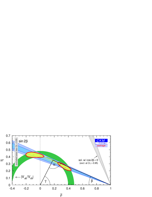
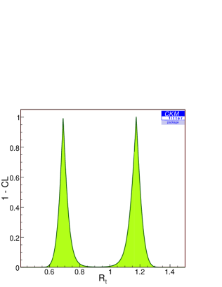
Figure 1: Results of the MFV fit I. See Table 2 for the constraints used. Left panel displays the selected area in the $(\overline{\rho}-\overline{\eta})$ plane, and the UT from the SM fit (2) is shown as reference. All contours are at 95% CL. Right panel reports the corresponding confidence level profile for $R_{t}$.

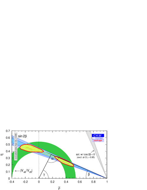
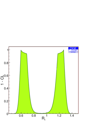
Figure 2: Results of the MFV fit II. See Table 2 for the constraints used. Left and right panels as in Fig. 1.

The $R_{t}$ values resulting from the fits of Figs. 1-2 are the following (95% CL)

$$(R_{t}^{(1)})_{\rm MFV-I}\in[0.62,0.78]~{},~{}~{}~{}(R_{t}^{(2)})_{\rm MFV-I}\in[1.07,1.26]~{},$$ (6)

$$(R_{t}^{(1)})_{\rm MFV-II}\in[0.54,0.79]~{},~{}~{}~{}(R_{t}^{(2)})_{\rm MFV-II}\in[1.06,1.34]~{}.$$ (7)

These values should be contrasted with the SM result for $R_{t}$, given in eq. (2). Some comments are in order here.

• In the MFV fit II, the inclusion of only $|V_{ub}|^{\rm(incl)}$ determines two disjoint solutions for $R_{t}$ (eq. (7)), which display a discrepancy with respect to the SM solution (eq. (2)), at more than the 2$\sigma$ level.

• The presence of two disjoint solutions for $R_{t}$ is featured also by the MFV fit I, where both the $|V_{ub}|^{\rm(incl)}$ and $|V_{ub}|^{\rm(excl)}$ determinations are included.

• The two $R_{t}$ solutions turn out to be even better resolved in the MFV fit I. This is due to the inclusion in the fit of the exclusive determinations for both $|V_{ub}|$ and $|V_{cb}|$. In fact, on the one hand, the latter would shift the central value for the average of $|V_{ub}|/|V_{cb}|$ respectively down and up, as compared to the value obtained in the MFV fit II, and the two effects tend to cancel. On the other hand, the presence of two determinations for both $|V_{ub}|$ and $|V_{cb}|$ reduces the final $|V_{ub}|/|V_{cb}|$ error with respect to the MFV fit II case.

One possible approach to the above findings is to raise doubts on the $|V_{ub}|^{\rm(incl)}$ determination [30, 31] (see [32] for the exclusive approach and [33] for a very recent reanalysis). We observe, however, that the inclusive value for $|V_{ub}|$ results from an average among quite a large number of modes, and the latter display consistency among each other. So the average would definitely appear under control, were it not for the above mentioned (and well known) discrepancy with the $|V_{ub}|$ value preferred by the global SM fit, close to the exclusive determination.

In the following we will pursue the possibility that the $|V_{ub}|^{\rm(incl)}$ determination be the correct one, and answer the question whether the MFV MSSM can account for either of the discrepancies $(R_{t})_{\rm SM}-(R_{t}^{(1,2)})_{\rm MFV}$. In particular, for $(R_{t}^{(1,2)})_{\rm MFV}$ we will take the results from the MFV fit II, which are the most conservative. Our study addresses the eventuality that $|V_{ub}|$ should consolidate to a value above that required by the SM fit. Since such value should most probably lie somewhere in between the present exclusive and inclusive determinations, our study represents somehow the ‘limiting’ case of a ‘high’ $|V_{ub}|$ value.

We finally note that, since the MFV determination of the UT can rely only on a handful of reasonably known observables (at present those in Table 2), our study stresses the importance of an accurate determination of $|V_{ub}|$ and of the angles $\alpha$ and $\gamma$. Angle determinations are fortunately a major task of the LHCb program and later, hopefully, of the Super-B [9], which will also allow a precision determination of $|V_{ub}|$.

3 Corrections to $R_{t}$ within the MFV MSSM

3.1 General formula for $R_{t}$

In the previous Section, we have focused our attention on the determination of the UT side $R_{t}$. This is because $R_{t}$ can in turn be expressed in terms of the $B_{d}$ and $B_{s}$ mass differences $\Delta M_{d}$ and $\Delta M_{s}$. For large $\tan\beta$, these quantities can undergo large SUSY corrections even in MFV [34]. To display the ‘dependence’ of $R_{t}$ on NP contributions to $\Delta M_{d,s}$, we write the following chain of equalities [6], starting from the very $R_{t}$ definition

$$R_{t}\equiv\frac{|V_{td}V_{tb}^{*}|}{|V_{cd}V_{cb}^{*}|}\cong\frac{1}{\lambda}\left|\frac{V_{td}}{V_{cb}}\right|=\frac{\xi}{\lambda}\sqrt{\frac{m_{B_{s}}}{m_{B_{d}}}}\left(\sqrt{\frac{\Delta M_{d}}{\Delta M_{s}}}\right)_{\rm SM}~{}.$$ (8)

In presence of NP contributions to $\Delta M_{d,s}$, one can always write relations of the kind

$$\Delta M_{q}=\Delta M_{q}^{\rm SM}(1+f_{q})~{},~{}~{}~{}~{}q=d,s~{},$$ (9)

where the l.h.s. represents the full theoretical predictions for the mass differences, which must in turn be identified with the experimentally measured quantities, since we are supposing the presence of NP. Then, eq. (8) can be rewritten as [6, 35, 7]

$$R_{t} = \frac{\xi}{\lambda}\sqrt{\frac{m_{B_{s}}}{m_{B_{d}}}}\sqrt{\frac{\Delta M_{d}}{\Delta M_{s}}}\sqrt{\frac{1+f_{s}}{1+f_{d}}}$$ (10)

$$= 0.913\left[\frac{\xi}{1.23}\right]\sqrt{\frac{17.8/{\rm ps}}{\Delta M_{s}}}\sqrt{\frac{\Delta M_{d}}{0.507/{\rm ps}}}\sqrt{\frac{1+f_{s}}{1+f_{d}}}~{},$$

where in the last equality we have plugged in the experimental values for $\Delta M_{d,s}$.

In the light of eq. (10), we consider now the two solutions $R_{t}^{(1,2)}$ (see eq. (7)) from the MFV fit II of the previous Section. We want to address the question whether the discrepancy with respect to the SM solution can be accounted for within the MFV MSSM. This will be the case if shifts $f_{q}$ from eq. (9) are sufficiently large to correct eq. (10) by the required amount.

3.2 MFV MSSM with low $\tan\beta$

This case, corresponding to $\tan\beta\mathrel{\hbox to0.0pt{\raise 2.20013pt\hbox{$<$}\hss}{\lower 2.20013pt\hbox{$\sim$}}}10$, was addressed in detail in Ref. [7]. There it was found that corrections $f_{q}$ are positive and do not exceed a few percent. It was also stressed that corrections tend to display alignment between the $\Delta M_{d}$ and $\Delta M_{s}$ cases, since NP contributions from scalar operators able to distinguish between the $q=d,s$ channels come with a factor of $m_{b}m_{q}/M_{W}^{2}$ and are below the 1% level. Therefore, within the MFV MSSM at low $\tan\beta$, the ratio $f_{q}=\Delta M_{q}^{\rm NP}/\Delta M_{q}^{\rm SM}$ tends to be the same for the $d,s$ cases and deviations on eq. (10) are not sufficient to reproduce the $R_{t}$ solutions of eq. (7).

3.3 MFV MSSM with large $\tan\beta$

Within the MSSM at large $\tan\beta$, the formulae for $\Delta M_{d}$ and $\Delta M_{s}$ feature also contributions from the so-called Higgs double penguins (DP), with exchange of $h_{0},H_{0}$ and $A_{0}$ bosons. For values of $\tan\beta\mathrel{\hbox to0.0pt{\raise 2.20013pt\hbox{$>$}\hss}{\lower 2.20013pt\hbox{$\sim$}}}30$, and assuming MFV, the $H_{0}$ and $A_{0}$ double penguins usually provide the dominant NP contribution which is found to be negative in the whole part of the SUSY parameter space with $M_{A}\in[200,500]$ GeV [36, 37, 38, 34]. The proportionality of such contribution to the external quark masses makes it generically negligible for the $\Delta M_{d}$ case, while for $\Delta M_{s}$ sizable corrections are possible.

In order to address the question whether the SUSY corrections to $\Delta M_{d}$ and $\Delta M_{s}$, computed in the MFV MSSM at large $\tan\beta$, can produce the shifts required for $R_{t}$ to reach any of the solutions in eq. (7), we adopt the following strategy

• compute the SUSY contributions to $\Delta M_{d,s}$ in the MSSM with large $\tan\beta$;

• perform the MFV limit, according to the EFT definition [3];

• study the quantity $(1+f_{d})/(1+f_{s})$ in the SUSY parameter space left after the MFV limit.

Concerning point 1, the calculation can be accomplished following the procedure of Ref. [34], which allows for a resummation of large $\tan\beta$ corrections. For a detailed description of this procedure, we refer to Section 2 of [34]. We mention that in our numerical analysis we consistently take into account effects coming from flavour off-diagonal squark mass matrices. We do not include, instead, effects arising from large $\tan\beta$ corrections to the Higgs propagator entering DP contributions. The latter corrections were found to have a non-negligible effect only for $M_{A}\lesssim 160$ GeV [39]. Similar conclusions will be drawn in Ref. [40]. Since we do not consider such light pseudoscalar Higgs masses in our numerical analysis, these new effects do not change the basic findings of the present work.

Turning to point 2, the MFV limit was performed in exact analogy with Ref. [7]. In particular we expand the soft terms, which enter the squark mass matrices, as functions of the SM Yukawa couplings. After such expansions, the soft terms are still parametrically dependent on an overall normalization mass scale and on the dimensionless coefficients tuning the proportionality to the Yukawa couplings themselves.

Finally, let us go to point 3. From the above discussion, it is clear that the SUSY parameters one needs to consider in the analysis are the same as in the low $\tan\beta$ case, with the addition of the neutral physical Higgs masses, entering the DP contributions. In order to have accurate numerical predictions for such masses, we used the package FeynHiggs [41, 42, 43, 44], which calculates the whole physical Higgs spectrum. The only additional parameter required by FeynHiggs besides those already present in the low $\tan\beta$ case is $M_{A}$. Consequently, in the notation of [7], parameters are

$$\overline{m}~{},~{}~{}A~{},~{}~{}M_{1}~{},~{}~{}M_{2}~{},~{}~{}M_{\tilde{g}}~{},$$ (11)

$$\mu~{},~{}~{}M_{A}~{},~{}~{}\tan\beta~{},$$ (12)

with the addition of the 12 ‘MFV coefficients’, governing the proportionality of the soft terms to the SM Yukawa couplings (see [7]). We observe that all these parameters are real, since the presence of complex phases would induce non-CKM CP violation in meson mixings. The latter would then contradict the MFV hypothesis.

To explore the SUSY parameter space, we adopt the following strategy. We study the ratio $(1+f_{s})/(1+f_{d})$, which enters $R_{t}$ in eq. (10), by generating the MFV coefficients with flat distributions in the same ranges as [7] (these ranges are also collected in Table 3).

Concerning the parameters in eqs. (11)-(12), we make the following observation. For large $\tan\beta$, box contributions are in general much smaller than the DP ones; in addition, the ‘alignment’ of the NP box contributions between the $\Delta M_{d,s}$ cases, stressed in Section 3.2, is found to hold for large $\tan\beta$ as well. As a consequence, when DP contributions are small, one has $(1+f_{s}^{\rm box})/(1+f_{d}^{\rm box})\approx 1$; conversely, when DP contributions are large, box corrections are just a small correction, with negligible modifications of the distribution shape.

Uniformly distributed	Fixed
$a_{1,2,3}\in[0.25,1]$	$\tan\beta=\{30,50\}$
$a_{4,5},b_{1,...,8}\in[-1,1]$	$M_{A}=\{200,500,800\}$ GeV
$A\in[-2,2]$ TeV	$\overline{m}=1$ TeV
$|\mu|\in[0.2,2]$ TeV	$M_{1}=M_{2}=500$ GeV
	$M_{\tilde{g}}=\{200,500,800\}$ GeV

Table 3: Parameter choices made in our scans. For the definition of the MFV coefficients $a_{i},b_{j},$ as well as of the squark biliear and trilinear mass scales $\overline{m}$ and $A$, see Ref. [7].

For the reason above, and as already stressed in Section 3.2, box contributions alone are not able to account for the $R_{t}$ solutions given in eq. (7). In order to address the analogous possibility for the double penguins, we set $\overline{m}=1$ TeV, thus decoupling box contributions, which would partially cancel the (dominant) DP corrections. Parameters $A$ and $|\mu|$ are instead generated flatly in the ranges $A\in[-2,+2]$ TeV and $|\mu|\in[0.2,2]$ TeV. On the sign of $\mu$ we will come back in the following discussion. The choice of the EW gaugino mass parameters plays a negligible role and we set them as $M_{1}=M_{2}=500$ GeV. Finally, we considered three discrete values for the gluino mass, namely $M_{\tilde{g}}=\{200,500,800\}$ GeV. Our results turn out to bear negligible dependence also on the choice of the gluino mass: we will further comment on this in due course. In our plots, the value $M_{\tilde{g}}=500$ GeV is chosen for definiteness.

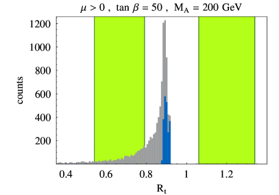
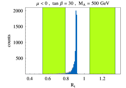
Figure 3: Distributions of values for $R_{t}$, resulting after scanning $A$, $|\mu|$ and the MFV parameters (see text for details). The left panel corresponds to $\mu>0$, $M_{A}=200$ GeV and $\tan\beta=50$; the right panel corresponds to $\mu<0$, $M_{A}=500$ GeV and $\tan\beta=30$. The grey (blue) distributions are without (with) the constraint (13). The vertical green bands correspond to the $R_{t}$ solutions given in eq. (7).

On the other hand, the quantity $(1+f_{s})/(1+f_{d})$ bears obviously a strong dependence on the choice of the mass $M_{A}$ (which also sets the scale for the $H_{0}$ DP) and on the value of $\tan\beta$. We have explored, in discrete steps, the ranges $M_{A}\in[200,800]$ GeV and $\tan\beta\in\{30,50\}$.

This completes the description of the choices made for the various SUSY parameters in our MonteCarlo study. These choices are also summarized in Table 3. In Fig. 3 we show as grey distributions the implied effects on $R_{t}$ for choices of $M_{A}$ and $\tan\beta$ where such effects are significant. The left panel corresponds to the choice $M_{A}=200$ GeV, $\tan\beta=50$ and $\mu>0$, while the right panel corresponds to $M_{A}=500$ GeV, $\tan\beta=30$ and $\mu<0$.

Here we note that, from the left panel of Fig. 3, the long tail looks able to reproduce the lower $R_{t}$ solution given in eq. (7). However, a large portion of the tail is actually unphysical, since it corresponds to values of $\Delta M_{s}$ which are outside the range allowed by the theoretical error ($\Delta M_{d}$ is only weakly affected by NP contributions, as we saw at the beginning of this section). When calculating $R_{t}$ out of $\Delta M_{d}^{\rm MSSM}$ and $\Delta M_{s}^{\rm MSSM}$, one should in fact take into account the constraints coming from the $\Delta M_{q}$ measurements. However, these constraints are by far dominated by the corresponding theoretical error. We stress that, in our case, the latter must take into account not only the uncertainty coming from the lattice parameters, but also the error associated with the CKM entries. For these entries one must in fact consistently use the determinations coming from the MFV fit, whose associated error is larger than that resulting from the usual SM fit determination.

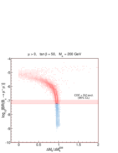
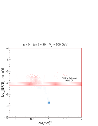
Figure 4: Correlation between BR$(B_{s}\to\mu^{+}\mu^{-})$ and $\Delta M_{d,s}$ in the MFV MSSM at large $\tan\beta$. Parameters as in Fig. 3.

The largeness of the final theoretical error makes then the $\Delta M_{q}$ constraints not very effective. We decided not to include this ‘filter’, since a much more effective one is provided by the BR$(B_{s}\to\mu^{+}\mu^{-})$ upper bound. The latest combined bound from the CDF and DØ collaborations reads [46]

$${\rm BR}(B_{s}\to\mu^{+}\mu^{-})<5.8\times 10^{-8}~{},~{}~{}~{}~{}\mbox{[95\% CL]}~{}.$$ (13)

The distribution of values for $R_{t}$ which survives the $B_{s}\to\mu^{+}\mu^{-}$ constraint is shown in blue in Fig. 3. For positive $\mu$, the constraint completely excludes the possibility of significant corrections to $R_{t}$, and sets the latter back to a SM-like value. For negative $\mu$ a similar conclusion holds, considering that less than 1% of the MC-generated values for $R_{t}$ lie within the 2$\sigma$ band of the lower $R_{t}$ solution, after the constraint (13) has been taken into account. We note that our results in Fig. 3 can be directly compared with Fig. 3 of [39], which reports the quantity $R_{sd}=(\Delta M_{s}/\Delta M_{s}^{\rm SM})/(\Delta M_{d}/\Delta M_{d}^{\rm SM})$. The latter is related to $R_{t}$ through $R_{t}=0.913\times\sqrt{R_{sd}}$. One can see that our MonteCarlo allows slightly larger maximal effects than in the case of [39]. This is most likely due to the fact that we do not include the constraints from $\overline{B}\to X_{s}\gamma$ and $B\to\tau\nu$, in constrast to Ref. [39]. Including these constraints would however only strenghten our conclusions.

The severeness of the constraint (13) on the allowed MFV MSSM corrections to $\Delta M_{s}$ is shown in Fig. 4. The latter reports the correlation [38] between BR$(B_{s}\to\mu^{+}\mu^{-})$ and $\Delta M_{s}$ in the MFV MSSM at large $\tan\beta$, that is roughly given by

$$\Delta M_{s}^{\rm DP}\propto-\left(\frac{M_{A}}{\tan\beta}\right)^{2}{\rm BR}(B_{s}\to\mu^{+}\mu^{-})~{}.$$ (14)

An interesting aspect of the above correlation is that, in the regime of DP dominance, a large part of the dependence on SUSY parameters other than $\tan\beta$ and $M_{A}$ cancels, since it is common to BR$(B_{s}\to\mu^{+}\mu^{-})$ and $\Delta M_{s}$. This is in particular true of the ‘$\epsilon$-factors’ $\epsilon_{Y},\tilde{\epsilon}_{3}$ and $\epsilon_{0}$ (compare eqs. (6.25) and (6.40) of Ref. [34]), which incorporate the dependence on the SUSY particles entering the loops. This explains, for example, the negligible dependence of the correlation (14) on the choice of the gluino mass, already mentioned in the discussion of the parameter ranges for the MonteCarlo. A similar finding holds for the $R_{t}$-distributions of Fig. 3, once the $B_{s}\to\mu^{+}\mu^{-}$ bound is taken into account.

In Fig. 4, we show two representative cases for the correlation (14). As stated previously in the text, parameters are chosen in order to have large (correlated) effects. For positive $\mu$, Fig. 4 (left panel) shows that the bound (13) basically excludes effects on $\Delta M_{s}$ exceeding $-10$%. In addition, the correlation with the prediction on $B_{s}\to\mu^{+}\mu^{-}$ is largely lost in the allowed region.

For negative $\mu$, neutral Higgs contributions to both BR$(B_{s}\to\mu^{+}\mu^{-})$ and $\Delta M_{s}$ are generically larger than in the corresponding positive $\mu$ case. Furthermore, according to eq. (14), one can choose larger values for $M_{A}$ and/or lower values for $\tan\beta$ in order to have a large correction to $\Delta M_{s}$ while fulfilling the constraint on BR$(B_{s}\to\mu^{+}\mu^{-})$. In Fig. 4 (right panel) we report a case with these features, corresponding to $\tan\beta=30$ and $M_{A}=500$ GeV. In fact, for negative values of $\mu$, one needs $M_{A}\gtrsim 500$ GeV if $\tan\beta\gtrsim 30$ in order to observe a significant correlated effect between $\Delta M_{s}$ and BR$(B_{s}\to\mu^{+}\mu^{-})$. One should also keep in mind that for $\mu<0$ the MSSM worsens the $(g-2)_{\mu}$ discrepancy with respect to the SM [49, 50].

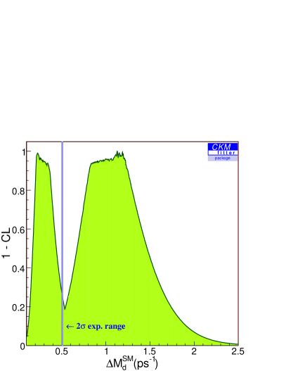
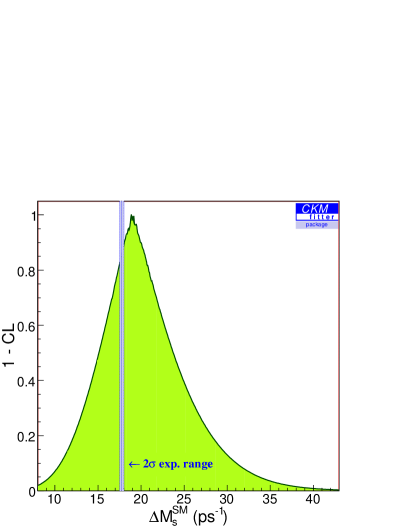
Figure 5: CL profiles for $\Delta M_{d}^{\rm SM}$ (left panel) and $\Delta M_{s}^{\rm SM}$ (right panel) for the MFV fit II.

We note here some peculiar features of the MFV MSSM corrections to $\Delta M_{d,s}$, which make them unable to reproduce any of the two $R_{t}$ solutions (7).

• Among the CKM elements entering the SM formulae for $\Delta M_{d,s}$, only $V_{td}$ is significantly modified within the MFV fit with respect to $V_{td}^{\rm SM}$. Since $V_{td}$ enters only $\Delta M_{d}$, in order to reproduce the experimental values one would need a correspondingly large correction $f_{d}$ on $\Delta M_{d}^{\rm SM}$ and a negligible $f_{s}$ correction to $\Delta M_{s}^{\rm SM}$. The MFV MSSM tends instead to give large corrections only to $\Delta M_{s}$. In fact DP contributions are sensitive to the external quark masses, and NP effects scale as $m_{q}m_{b}$ for $\Delta M_{q}$.

• In absence of the BR$(B_{s}\to\mu^{+}\mu^{-})$ constraint, corrections to $R_{t}$ tend to reproduce the lower solution, since $f_{s}$ in eq. (10) is negative. On the other hand, the higher solution looks the favored one, e.g. by the tree-level determination for the angle $\gamma$.

Concerning point a, we show in Fig. 5 the CL profiles for $\Delta M_{d,s}^{\rm SM}$ within the MFV fit II. As one can see, in this case the SM formula for $\Delta M_{d}$ favors two solutions, corresponding to the shifts in the values of $V_{td}$. On the other hand, $\Delta M_{s}^{\rm SM}$ is perfectly compatible with the experimental result.

We have studied the distribution of values for $R_{t}$ as given in eq. (10) for different choices of the relevant low-energy parameter $\xi$, which brings the largest contribution to the overall error. Results are displayed in the left panels of Fig. 6. In addition, when assuming MFV, a distribution of values for $R_{t}$ can be translated into a corresponding distribution for $\gamma$, with the only additional uncertainty of $\sin 2\beta$, to which however $\gamma$ is only weakly sensitive. Then, similarly to $R_{t}$, one can study the dependence of the $\gamma$ determination on the value of $\xi$. Results are shown in the right panels of Fig. 6. The two solutions for $\gamma$ corresponding to the $R_{t}$ determinations of eq. (7) are as follows (95% CL)

$$(\gamma^{(1)})_{\rm MFV-II}=[21,48]^{\circ}~{},~{}~{}~{}(\gamma^{(2)})_{\rm MFV-II}=[87,120]^{\circ}~{}.$$ (15)

They are displayed in Fig. 6 (right) as horizontal green bands.

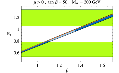
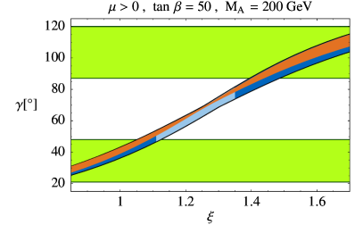
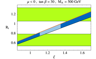
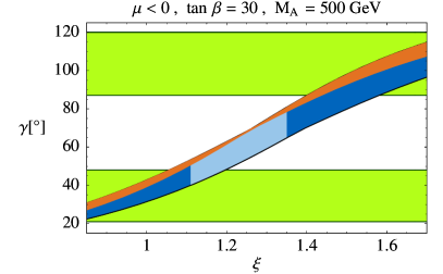
Figure 6: $R_{t}$ vs. $\xi$ and $\gamma$ vs. $\xi$ plots for $\mu>0$ (high panels) and $\mu<0$ (low panels). The blue bands represent the range of values allowed within the MFV MSSM. The central superimposed light blue belts correspond to the present 2$\sigma$-range for $\xi$ from lattice QCD (see Table 1). The orange lines report the SM results. Finally the two horizontal green bands represent the $R_{t}$ (left panels) or $\gamma$ (right panels) solutions from the MFV fit II, eqs. (7) and (15).

We conclude this Section by noting that further support to the above results is provided by studying the quantity $\epsilon_{K}$. The latter presents features exactly analogous to $\Delta M_{d}$. In particular: (i) given its dependence on $V_{td}$, in the MFV fits the SM formula gives two solutions; (ii) to reproduce the experimental value, one would need relatively large NP contributions; (iii) within the MFV MSSM, such contributions are however negligible in the full parameter space, so that agreement would again require the parameter $B_{K}$ to be substantially different ($>2\sigma$) from the present lattice determination.

4 Conclusions

In the present paper we have pointed out that the large value of $|V_{ub}|$ from inclusive tree-level determinations is not only a challenge for the Standard Model, but also for the MSSM with MFV. The patterns and the size of modifications of $\Delta M_{d}$ and $\Delta M_{s}$ in the MSSM with MFV do not allow a consistent description of the data in this case, unless very significant modifications of non-perturbative parameters determinations relative to the lattice ones are made. Concerning in particular the modifications allowed to $\Delta M_{s}$, we conclude that scenarios with 200 GeV $\lesssim M_{A}\lesssim$ 500 GeV and $\tan\beta\simeq 50$ that predict a significant suppression for $\Delta M_{s}$ in correlation with an enhancement for BR$(B_{s}\to\mu^{+}\mu^{-})$ have to be fine-tuned in order not to violate the new combined bound on the latter decay mode from the CDF and DØ collaborations. Relatively large correlated effects can however still occur for negative values of $\mu$ and large values for $M_{A}\gtrsim 500$ GeV, increasing with increasing $\tan\beta\gtrsim 30$.

The resolution of the $|V_{ub}|$ problem – that is, the discrepancy between the exclusive and inclusive determinations of this quantity – calls in the first place for a better theoretical control on the relevant hadronic quantities involved in either determination. If the two determinations should then agree on a central value in the ballpark of the present inclusive average, insight on the tension existing within the SM and the MFV MSSM will require a facility like Super-B [9], where also a very precise determination of the angle $\gamma$ from tree-level processes is possible. As we have seen, the precise knowledge of this angle could definitely tell us whether MSSM with MFV has a chance to be a correct description of flavour violating processes.

References

- [1] L. J. Hall and L. Randall, Weak scale effective supersymmetry, Phys. Rev. Lett. 65 (1990) 2939–2942.
- [2] R. S. Chivukula and H. Georgi, Composite technicolor Standard Model, Phys. Lett. B188 (1987) 99.
- [3] G. D’Ambrosio, G. F. Giudice, G. Isidori, and A. Strumia, Minimal flavour violation: An effective field theory approach, Nucl. Phys. B645 (2002) 155–187, [hep-ph/0207036].
- [4] A. J. Buras, P. Gambino, M. Gorbahn, S. Jager, and L. Silvestrini, Universal unitarity triangle and physics beyond the Standard Model, Phys. Lett. B500 (2001) 161–167, [hep-ph/0007085].
- [5] A. J. Buras, Minimal flavor violation, Acta Phys. Polon. B34 (2003) 5615–5668, [hep-ph/0310208]. Lectures given at 43rd Cracow School of Theoretical Physics, Zakopane, Poland, 30 May - 9 Jun 2003.
- [6] M. Blanke, A. J. Buras, D. Guadagnoli, and C. Tarantino, Minimal flavour violation waiting for precise measurements of , , , , and , JHEP 10 (2006) 003, [hep-ph/0604057].
- [7] W. Altmannshofer, A. J. Buras, and D. Guadagnoli, The MFV limit of the MSSM for low : meson mixings revisited, hep-ph/0703200.
- [8] G. Isidori, F. Mescia, P. Paradisi, C. Smith, and S. Trine, Exploring the flavour structure of the MSSM with rare K decays, JHEP 08 (2006) 064, [hep-ph/0604074].
- [9] SuperB, Conceptual Design Report, INFN/AE-07/2, SLAC-R-856, LAL 07-15, available at http://www.pi.infn.it/SuperB/?q=CDR.
- [10] UTfit website: http://www.utfit.org.
- [11] UTfit Collaboration, M. Bona et al., The UTfit collaboration report on the unitarity triangle beyond the standard model: Spring 2006, Phys. Rev. Lett. 97 (2006) 151803, [hep-ph/0605213].
- [12] UTfit Collaboration, M. Bona et al., The UTfit collaboration report on the status of the unitarity triangle beyond the standard model. I: Model- independent analysis and minimal flavour violation, JHEP 03 (2006) 080, [hep-ph/0509219].
- [13] A. J. Buras, R. Fleischer, S. Recksiegel, and F. Schwab, , new physics in and implications for rare and decays, Phys. Rev. Lett. 92 (2004) 101804, [hep-ph/0312259].
- [14] CKMfitter website: http://ckmfitter.in2p3.fr.
- [15] A. Hocker, H. Lacker, S. Laplace, and F. Le Diberder, A new approach to a global fit of the CKM matrix, Eur. Phys. J. C21 (2001) 225–259, [hep-ph/0104062].
- [16] S. Hashimoto, Recent results from lattice calculations, Int. J. Mod. Phys. A20 (2005) 5133–5144, [hep-ph/0411126].
- [17] Heavy Flavor Averaging Group (HFAG) Collaboration, E. Barberio et al., Averages of b-hadron properties at the end of 2006, arXiv:0704.3575 [hep-ex].
- [18] B. O. Lange, M. Neubert, and G. Paz, Theory of charmless inclusive B decays and the extraction of , Phys. Rev. D72 (2005) 073006, [hep-ph/0504071].
- [19] S. W. Bosch, B. O. Lange, M. Neubert, and G. Paz, Factorization and shape-function effects in inclusive B- meson decays, Nucl. Phys. B699 (2004) 335–386, [hep-ph/0402094].
- [20] S. W. Bosch, M. Neubert, and G. Paz, Subleading shape functions in inclusive B decays, JHEP 11 (2004) 073, [hep-ph/0409115].
- [21] M. Neubert, Impact of four-quark shape functions on inclusive B decay spectra, Eur. Phys. J. C44 (2005) 205–209, [hep-ph/0411027].
- [22] M. Neubert, Two-loop relations for heavy-quark parameters in the shape- function scheme, Phys. Lett. B612 (2005) 13–20, [hep-ph/0412241].
- [23] J. R. Andersen and E. Gardi, Inclusive spectra in charmless semileptonic B decays by dressed gluon exponentiation, JHEP 01 (2006) 097, [hep-ph/0509360].
- [24] C. W. Bauer, Z. Ligeti, and M. E. Luke, Precision determination of from inclusive decays, Phys. Rev. D64 (2001) 113004, [hep-ph/0107074].
- [25] P. Ball and R. Zwicky, New results on decay formfactors from light-cone sum rules, Phys. Rev. D71 (2005) 014015, [hep-ph/0406232].
- [26] A. Abada et al., Heavy light semileptonic decays of pseudoscalar mesons from lattice QCD, Nucl. Phys. B619 (2001) 565–587, [hep-lat/0011065].
- [27] E. Dalgic et al., B Meson Semileptonic Form Factors from Unquenched Lattice QCD, Phys. Rev. D73 (2006) 074502, [hep-lat/0601021].
- [28] W.-M. Yao et al., Review of Particle Physics, Journal of Physics G 33 (2006) 1+.
- [29] CDF Collaboration, A. Abulencia et al., Observation of oscillations, Phys. Rev. Lett. 97 (2006) 242003, [hep-ex/0609040].
- [30] P. Ball, from the Spectrum of , arXiv:0705.2290 [hep-ph].
- [31] P. Gambino, P. Giordano, G. Ossola, and N. Uraltsev, Inclusive semileptonic B decays and the determination of , arXiv:0707.2493 [hep-ph].
- [32] M. C. Arnesen, B. Grinstein, I. Z. Rothstein, and I. W. Stewart, A precision model independent determination of from , Phys. Rev. Lett. 95 (2005) 071802, [hep-ph/0504209].
- [33] J. M. Flynn and J. Nieves, from exclusive semileptonic decays revisited, arXiv:0705.3553 [hep-ph].
- [34] A. J. Buras, P. H. Chankowski, J. Rosiek, and L. Slawianowska, , and in supersymmetry at large , Nucl. Phys. B659 (2003) 3, [hep-ph/0210145].
- [35] P. Ball and R. Fleischer, Probing new physics through B mixing: Status, benchmarks and prospects, Eur. Phys. J. C48 (2006) 413–426, [hep-ph/0604249].
- [36] A. J. Buras, P. H. Chankowski, J. Rosiek, and L. Slawianowska, , and the angle in the presence of new operators, Nucl. Phys. B619 (2001) 434–466, [hep-ph/0107048].
- [37] G. Isidori and A. Retico, Scalar flavour-changing neutral currents in the large- limit, JHEP 11 (2001) 001, [hep-ph/0110121].
- [38] A. J. Buras, P. H. Chankowski, J. Rosiek, and L. Slawianowska, Correlation between and in supersymmetry at large , Phys. Lett. B546 (2002) 96–107, [hep-ph/0207241].
- [39] A. Freitas, E. Gasser, and U. Haisch, Supersymmetric large corrections to and revisited, hep-ph/0702267.
- [40] M. Gorbahn, S. Jager, U. Nierste and S. Trine. In preparation.
- [41] S. Heinemeyer, W. Hollik, and G. Weiglein, FeynHiggs: A program for the calculation of the masses of the neutral CP-even Higgs bosons in the MSSM, Comput. Phys. Commun. 124 (2000) 76–89, [hep-ph/9812320].
- [42] S. Heinemeyer, W. Hollik, and G. Weiglein, The masses of the neutral CP-even Higgs bosons in the MSSM: Accurate analysis at the two-loop level, Eur. Phys. J. C9 (1999) 343–366, [hep-ph/9812472].
- [43] G. Degrassi, S. Heinemeyer, W. Hollik, P. Slavich, and G. Weiglein, Towards high-precision predictions for the MSSM Higgs sector, Eur. Phys. J. C28 (2003) 133–143, [hep-ph/0212020].
- [44] M. Frank et al., The Higgs boson masses and mixings of the complex MSSM in the Feynman-diagrammatic approach, JHEP 02 (2007) 047, [hep-ph/0611326].
- [45] M. Carena, A. Menon, and C. E. M. Wagner, Challenges for MSSM Higgs searches at Hadron Colliders, arXiv:0704.1143 [hep-ph].
- [46] See talk by A. Maciel at HEP 2007, Parallel Session “Flavour Physics and CP Violation”, July 20, 2007.
- [47] http://www-cdf.fnal.gov/physics/new/bottom/060316.blessed-bsmumu3 and CDF Public note 8176.
- [48] J. Foster, K.-I. Okumura, and L. Roszkowski, New constraints on SUSY flavour mixing in light of recent measurements at the Tevatron, Phys. Lett. B641 (2006) 452–460, [hep-ph/0604121].
- [49] G. Isidori and P. Paradisi, Hints of large in flavour physics, Phys. Lett. B639 (2006) 499–507, [hep-ph/0605012].
- [50] G. Isidori, F. Mescia, P. Paradisi, and D. Temes, Flavour physics at large with a Bino-like LSP, Phys. Rev. D75 (2007) 115019, [hep-ph/0703035].