Design of optimal convolutional codes for joint decoding of correlated sources in wireless sensor networks

Abstract

We consider a wireless sensors network scenario where two nodes detect correlated sources and deliver them to a central collector via a wireless link. Differently from the Slepian-Wolf approach to distributed source coding, in the proposed scenario the sensing nodes do not perform any pre-compression of the sensed data. Original data are instead independently encoded by means of low-complexity convolutional codes. The decoder performs joint decoding with the aim of exploiting the inherent correlation between the transmitted sources. Complexity at the decoder is kept low thanks to the use of an iterative joint decoding scheme, where the output of each decoder is fed to the other decoder’s input as a-priori information. For such scheme, we derive a novel analytical framework for evaluating an upper bound of joint-detection packet error probability and for deriving the optimum coding scheme. Experimental results confirm the validity of the analytical framework, and show that recursive codes allow a noticeable performance gain with respect to non-recursive coding schemes. Moreover, the proposed recursive coding scheme allows to approach the ideal Slepian-Wolf scheme performance in AWGN channel, and to clearly outperform it over fading channels on account of diversity gain due to correlation of information.

Index Terms – Convolutional codes, correlated sources, joint decoding, wireless sensor networks.

I Introduction

Wireless sensor networks have recently received a lot of attention in the research literature [1]. The efficient transmission of correlated signals observed at different nodes to one or more collectors, is one of the main challenges in such networks. In the case of one collector node, this problem is often referred to as reach-back channel in the literature [2], [3], [4]. In its most simple form, the problem can be summarized as follows: two independent nodes have to transmit correlated sensed data to a collector node by using the minimum energy, i.e., by exploiting in some way the implicit correlation among data. In an attempt to exploit such correlation, many works have recently focussed on the design of coding schemes that approach the Slepian-Wolf fundamental limit on the achievable compression rates [5], [6], [7], [8]. However, approaching the Slepian-Wolf compression limit requires in general a huge implementation complexity at the transmitter (in terms of number of operations and memory requirements) that in many cases is not compatible with the needs of deploying very light-weight, low cost, and low consuming sensor nodes. Alternative approaches to distributed source coding are represented by cooperative source-channel coding schemes and joint source-channel coding.

In a cooperative system, each user is assigned one or more partners. The partners overhear each other’s transmitted signals, process these signals, and retransmit toward the destination to provide extra observations of the source signal at the collector. Even though the inter partner channel is noisy, the virtual transmit-antenna array consisting of these partners provides additional diversity, and may entail improvements in terms of error rates and throughput for all the nodes involved [9], [10], [11], [12] [13], [14]. This approach can take advantage of correlation among the different information flows simply by including Slepian-Wolf based source coding schemes, i.e., the sensing nodes transmit compressed version of the sensed data each other, so that cooperative source-channel coding schemes can be derived [15]. However, approaches based on cooperation require a strict coordination/synchronization among nodes, so that they can be considered as a single transmitter equipped with multiple antennas. This entails a more complex design of low level protocols and forces the nodes to fully decode signals from the other nodes. This operation is of course power consuming, and in some cases such an additional power can partially or completely eliminate the advantage of distributed diversity.

An alternative solution to exploit correlation among users is represented by joint source-channel coding. In this case, no cooperation among nodes is required and the correlated sources are not source encoded but only channel encoded at a reduced rate (with respect to the uncorrelated case). The reduced reliability due to channel coding rate reduction can be compensated by exploiting intrinsic correlation among different information sources at the channel decoder. Such an approach has attracted the attention of several researchers in the recent past on account of its implementation simplicity [16], [17], [18], [19]. Works dealing with joint source-channel coding have so far considered classical turbo or LDPC codes, where the decoder can exploit the correlation among sources by performing message passing between the two decoders. However, in order to exploit the potentialities of such codes it is necessary to envisage very long transmitted sequences (often in the order of 10000 bits or even longer), a situation which is not so common in wireless sensor networks’ applications where in general the nodes have to deliver a small packet of bits. Of course, the same encoding and decoding principles of turbo/LDPC codes can be used with shorter block lengths, but the decoder’s performance becomes in this case similar to that of classical block or convolutional codes.

In this paper, we will consider a joint source-channel coding scheme based on a low-complexity (i.e., small number of states) convolutional coding scheme. In this case, both the memory requirement at the encoder and the transmission delay are of very few bits (i.e., the constraint length of the code). Moreover, similarly to turbo or LDPC schemes, the complexity at the decoder can be kept low thanks to the use of an iterative joint decoding scheme, where the output of each decoder is fed to the other decoder’s input as a-priori information. It is worth noting that when a convolutional code is used to provide forward error correction for packet data transmissions, we are in general interested in the average probability of block (or packet) error rather than in the bit error rate [20].
In order to manage the problem complexity, we assume that a-priori information is ideal, i.e., it is identical to the original information transmitted by the other encoder. In this case, the correlation between the a-priori information and the to-be-decoded bits is still equal to the original correlation between the information signals, and the problem turns out to be that of Viterbi decoding with a-priori soft information.
To the best of my knowledge, the first paper which studies this problem is an old paper by Hagenauer [21]. The bounds found by Hagenauer are generally accepted by the research community, and a recent paper [22] uses such bounds to evaluate the performance of a joint convolutional decoding system similar to the one proposed in this paper. Unfortunately, the bounds found by Hagenauer are far from being satisfying, as we will show in Section IV. In particular, in [21] it is assumed a perfect match between the a-priori information hard decision parameter, i.e., the sign of the a-priori log-likelihood values, and the actually transmitted information signal. On the other hand, in [22] the good match between simulations and theoretical curves is due to the use of base-10 logarithm instead of the correct natural logarithm. Hence, this paper removes the assumptions made in [21] and a novel analytical framework, where the packet error probability is evaluated by averaging over all possible configuration of a-priori information, is provided. Such an analysis is then considered for deriving optimal coding schemes for the scenario proposed in this paper.

This paper is organized as follows. Section II describes the proposed scenario and gives notations used throughout the rest of the paper. In Section III, starting from the definition of the optimum MAP joint-decoding problem, we derive a sub-optimum iterative joint-decoding scheme. Section IV and V illustrate the analysis which allows to evaluate the packet error probabilities of convolutional joint-decoding and to derive the optimum code searching strategy. Finally, Section VI shows results and comparisons.

II Scenario

Let’s consider the detecting problem shown in Figure 1. We have two sensor nodes, namely $SN_{1}$ and $SN_{2}$, which detect the two binary correlated signals X and Y, respectively. Such signals, referred to as information signals in the following, are taken to be i.i.d. correlated binary randon variables with $P_{r}\left\{x_{i}=1/0\right\}=P_{r}\left\{y_{i}=1/0\right\}=0.5$ and correlation $\rho=P_{r}\left\{x_{i}=y_{i}\right\}>0.5$.
The information signals, which are assumed to be detectable without error (i.e., ideal sensor nodes), must be delivered to the access point node (AP). To this aim, sensor nodes can establish a direct link toward the AP. We assume that the communication links are affected by independent link gains and by additive AWGN noise. Referring to the vectorial equivalent low-pass signal representation, we denote to as ${\mathbf{s}}$ the complex transmitted vector which conveys the information signal, $\alpha$ the complex link gain term which encompasses both path loss and fading, and ${\mathbf{n}}$ the complex additive noise. As for the channel model, we assume an almost static system characterized by very slow fading, so that the channel link gains can be perfectly estimated at the receiver .

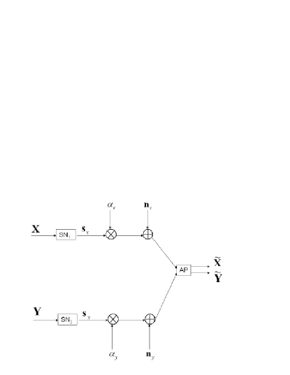
Figure 1: The proposed two sensing nodes scenario

Let’s assume that each transmitter uses a rate $r=k/n$ binary antipodal channel coding scheme to protect information from channel errors, and denote to as ${\mathbf{x}}=\left(x_{0},x_{1},\ldots,x_{k-1}\right)$ and ${\mathbf{z}}=\left(z_{0},z_{1},\ldots,z_{n-1}\right)$, with $z_{i}=\pm 1$, the information and the coded sequences for $SN_{1}$, respectively. In an analogous manner, ${\mathbf{y}}=\left(y_{0},y_{1},\ldots,y_{k-1}\right)$ and ${\mathbf{w}}=\left(w_{0},w_{1},\ldots,w_{n-1}\right)$, with $w_{i}=\pm 1$, are the information and the coded sequences for $SN_{2}$.
Eventually, let’s denote to as $E(\cdot)$ the mean operator and introduce the following terms: $\xi_{x}=E\left(\left|{\mathbf{s}}_{x}\right|^{2}/2\right)$, is the energy per coded sample transmitted by $SN_{1}$, $\xi_{y}=E\left(\left|{\mathbf{s}}_{y}\right|^{2}/2\right)$, is the energy per coded sample transmitted by $SN_{2}$, $G_{x}=\left|\alpha_{x}\right|^{2}$, is the power gain term for the first link, $G_{y}=\left|\alpha_{y}\right|^{2}$, is the power gain term for the second link, $E\left(\left|{\mathbf{n}}_{x}\right|^{2}\right)=E\left(\left|{\mathbf{n}}_{y}\right|^{2}\right)=2N_{0}$, is the variance of the AWGN noise.

The coded sequence is transmitted into the channel with an antipodal binary modulation scheme (PSK), i.e., $s_{x,i}=z_{i}\sqrt{2\xi_{x}}$, $s_{y,i}=w_{i}\sqrt{2\xi_{y}}$. Hence, denoting to as $u_{x,i}$ and $u_{y,i}$ the decision variable at the receiver, we get:

$$\begin{array}[]{c}u_{i,x}=z_{i}\sqrt{2G_{x}\xi_{x}}+\eta_{i,x}\\ u_{i,y}=w_{i}\sqrt{2G_{y}\xi_{y}}+\eta_{i,y}\end{array}$$ (1)

where $\eta_{i,x}$, $\eta_{i,y}$ are Gaussian random noise terms with zero mean and variance $N_{0}$. The energy per information bit for the two links can be written as $\xi_{b,x}=\frac{G_{x}\xi_{x}}{r}$ and $\xi_{b,y}=\frac{G_{y}\xi_{y}}{r}$, respectively. Denoting to as $\xi_{c,x}=r\xi_{b,x}$ and $\xi_{c,y}=r\xi_{b,y}$ the received energy per coded bit for the two links, we can rewrite equation (1) as:

$$\begin{array}[]{c}u_{i,x}=z_{i}\sqrt{2\xi_{c,x}}+\eta_{i,x}\\ u_{i,y}=w_{i}\sqrt{2\xi_{c,y}}+\eta_{i,y}\end{array}$$ (2)

Note that the same model attains also for a more efficient quaternary modulation scheme (QPSK), where two coded symbols are transmitted at the same time in the real and imaginary part of the complex transmitted sample.

III Iterative joint-decoding

The decoders’ problem is that of providing an estimation of ${\mathbf{x}}$ and ${\mathbf{y}}$ given the observation sequences ${\mathbf{u}}_{x}$ and ${\mathbf{u}}_{y}$. Since ${\mathbf{x}}$ and ${\mathbf{y}}$ are correlated, the optimum decoding problem can be addressed as a MAP joint decoding problem:

$$\begin{array}[]{cl}\left\{\tilde{{\mathbf{x}}},\tilde{{\mathbf{y}}}\right\}=\mathop{arg~{}max}\limits_{{{\mathbf{x}}},{{\mathbf{y}}}}Pr\left\{{{\mathbf{x}}},{{\mathbf{y}}}|{{\mathbf{u}}_{x}},{{\mathbf{u}}_{y}}\right\}\end{array}$$ (3)

where $\tilde{{\mathbf{x}}}$ and $\tilde{{\mathbf{y}}}$ are the jointly estimated information sequences.

Although its optimality, such a joint decoding scheme requires in general a huge computational effort to be implemented. As a matter of fact, it requires a squared number of operation per seconds with respect to unjoint decoding. Such an implementation complexity is expected in many cases to be too high, particularly when wireless sensor networks’ applications are of concern. In order to get a simplified receiver structure, let’s now observe that by using the Bayes rule equation (3) can be rewritten as:

$$\begin{array}[]{cl}\left\{\tilde{{\mathbf{x}}},\tilde{{\mathbf{y}}}\right\}=\mathop{arg~{}max}\limits_{{{\mathbf{x}}},{{\mathbf{y}}}}Pr\left\{{\mathbf{x}}|{\mathbf{y}},{{\mathbf{u}}_{x}},{{\mathbf{u}}_{y}}\right\}Pr\left\{{\mathbf{y}}|{{\mathbf{u}}_{x}},{{\mathbf{u}}_{y}}\right\}\end{array}$$ (4)

The above expression can be simplified by observing that ${{\mathbf{u}}_{y}}$ is e noisy version of ${\mathbf{y}}$ and that the noise is independent of ${\mathbf{x}}$. Hence, (4) can be rewritten as:

$$\begin{array}[]{cl}\left\{\tilde{{\mathbf{x}}},\tilde{{\mathbf{y}}}\right\}=\mathop{arg~{}max}\limits_{{{\mathbf{x}}},{{\mathbf{y}}}}Pr\left\{{\mathbf{x}}|{\mathbf{y}},{{\mathbf{u}}_{x}}\right\}Pr\left\{{\mathbf{y}}|{{\mathbf{u}}_{x}},{{\mathbf{u}}_{y}}\right\}\end{array}$$ (5)

By making similar considerations as above, it is straightforward to derive from (5) the equivalent decoding rule:

$$\begin{array}[]{cl}\left\{\tilde{{\mathbf{x}}},\tilde{{\mathbf{y}}}\right\}=\mathop{arg~{}max}\limits_{{{\mathbf{x}}},{{\mathbf{y}}}}Pr\left\{{\mathbf{y}}|{\mathbf{x}},{{\mathbf{u}}_{y}}\right\}Pr\left\{{\mathbf{x}}|{{\mathbf{u}}_{x}},{{\mathbf{u}}_{y}}\right\}\end{array}$$ (6)

Let’s now consider the following system of equations:

$$\begin{array}[]{cl}\tilde{{\mathbf{x}}}=\mathop{arg~{}max}\limits_{{{\mathbf{x}}}}Pr\left\{{\mathbf{x}}|{\tilde{\mathbf{y}}},{{\mathbf{u}}_{x}}\right\}Pr\left\{{\tilde{\mathbf{y}}}|{{\mathbf{u}}_{x}},{{\mathbf{u}}_{y}}\right\}\\ \tilde{{\mathbf{y}}}=\mathop{arg~{}max}\limits_{{{\mathbf{y}}}}Pr\left\{{\mathbf{y}}|\tilde{{\mathbf{x}}},{{\mathbf{u}}_{y}}\right\}Pr\left\{\tilde{{\mathbf{x}}}|{{\mathbf{u}}_{x}},{{\mathbf{u}}_{y}}\right\}\end{array}$$ (7)

It is straightforward to observe that the above system has at least one solution, that is the optimum MAP solution given by (5) or (6).
It is also worth noting that $Pr\left\{{\tilde{\mathbf{y}}}|{{\mathbf{u}}_{x}},{{\mathbf{u}}_{y}}\right\}$ and $Pr\left\{\tilde{{\mathbf{x}}}|{{\mathbf{u}}_{x}},{{\mathbf{u}}_{y}}\right\}$ are constant terms in (7). Therefore, the decoding problem (7) can be rewritten as:

$$\begin{array}[]{cl}\tilde{{\mathbf{x}}}=\mathop{arg~{}max}\limits_{{{\mathbf{x}}}}Pr\left\{{\mathbf{x}}|{\tilde{\mathbf{y}}},{{\mathbf{u}}_{x}}\right\}\\ \tilde{{\mathbf{y}}}=\mathop{arg~{}max}\limits_{{{\mathbf{y}}}}Pr\left\{{\mathbf{y}}|\tilde{{\mathbf{x}}},{{\mathbf{u}}_{y}}\right\}\end{array}$$ (8)

In (8) the decoding problem has been split into two sub-problems: in each sub-problem the decoder detects one information signal basing on a-priori information given by the other decoder. A-priori information will be referred to as side-information in the following.
A solution of the above problem could be obtained by means of an iterative approach, thus noticeably reducing the implementation complexity with respect to optimum joint decoding. However, demonstrating if the iterative decoding scheme converges and, if it does, to which kind of solution it converges, is a very cumbersome problem which is out of the scope of this paper. As in the traditional turbo decoding problem, we are instead interested in deriving a practical method to solve (8).

To this aim, classical Soft Input Soft Output (SISO) decoding schemes, where the decoder gets at its input a-priori information of input bits and produce at its output a MAP estimation of the same bits, can be straightforwardly used in this scenario. MAP estimations and a-priori information are often expressed as log-likelihood probabilities ratios, which can be easily converted in bit probabilities [23]. Let denote by $P_{I}\left\{x_{i}\right\}$ and $P_{I}\left\{y_{i}\right\}$ the a-priori probabilities at the SISO decoders’ inputs, and by $P_{O}\left\{x_{i}\right\}$ and $P_{O}\left\{y_{i}\right\}$ the a-posteriori probabilities evaluated by the two decoders. In order to let the iterative scheme working, it is necessary to convert a-posteriori probabilities evaluated at $j-th$ step into a-priori probabilities for the $(j+1)-th$ step. According to the correlation model between the information signals, we get:

$$\begin{array}[]{cl}P_{I}\left\{y_{i}\right\}=P_{O}\left\{x_{i}\right\}\times\rho+\left(1-P_{O}\left\{x_{i}\right\}\right)\times\left(1-\rho\right)\\ P_{I}\left\{x_{i}\right\}=P_{O}\left\{y_{i}\right\}\times\rho+\left(1-P_{O}\left\{y_{i}\right\}\right)\times\left(1-\rho\right)\end{array}$$ (9)

As for the decoding scheme, we consider the Soft Output Viterbi Decoding (SOVA) scheme depicted in [23]. Denoting to as $\Upsilon$ the SOVA decoding function, the overall iterative procedure can be summarized as:

$$\begin{array}[]{c}P^{(1)}_{I}\left\{x_{i}\right\}=0.5;\hfill\\ for~{}j~{}=~{}1,N\hfill\\ ~{}~{}~{}~{}P^{(j)}_{O}\left\{x_{i}\right\}=\Upsilon\left(P^{(j)}_{I}\left\{x_{i}\right\},{{\mathbf{u}}_{x}}\right);\hfill\\ ~{}~{}~{}~{}P^{(j)}_{I}\left\{y_{i}\right\}=P^{(j)}_{O}\left\{x_{i}\right\}\times\rho+\left(1-P^{(j)}_{O}\left\{x_{i}\right\}\right)\times\left(1-\rho\right);\hfill\\ ~{}~{}~{}~{}P^{(j)}_{O}\left\{y_{i}\right\}=\Upsilon\left(P^{(j)}_{I}\left\{y_{i}\right\},{{\mathbf{u}}_{y}}\right);\hfill\\ ~{}~{}~{}~{}P^{(j)}_{I}\left\{x_{i}\right\}=P^{(j)}_{O}\left\{y_{i}\right\}\times\rho+\left(1-P^{(j)}_{O}\left\{y_{i}\right\}\right)\times\left(1-\rho\right);\hfill\\ end;\hfill\end{array}$$ (10)

where $N$ is the number of iterations. In Figure 2 the iterative SOVA joint decoding scheme described above is depicted. We assume that the correlation factor $\rho$ between the information signals is perfectly known/estimated at the receiver. Such an assumption is reasonable since $\rho$ is expected to remain almost constant for long time.

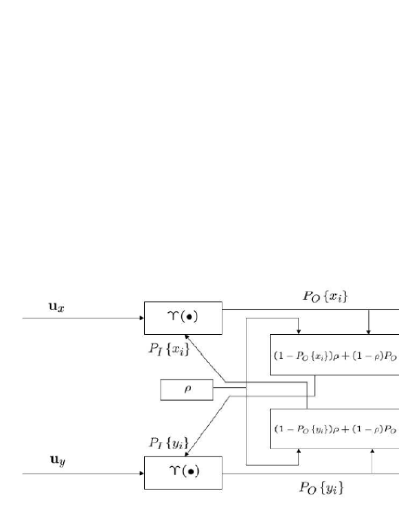
Figure 2: SOVA Iterative decoding scheme

IV Pairwise error probability

We now are interested in evaluating the performance of the iterative joint-decoding scheme. To this aim, we consider a simplified problem where the side-information provided to the other decoder is without errors, i.e., it is equal to the original information signal. Without loss of generality, let focus on the first decoder:

$$\begin{array}[]{cl}\tilde{{\mathbf{x}}}=\mathop{arg~{}max}\limits_{{{\mathbf{x}}}}Pr\left\{{\mathbf{x}}|\hat{{{\mathbf{y}}}},{{\mathbf{u}}_{x}}\right\}\end{array}$$ (11)

where $\hat{{{\mathbf{y}}}}$ is the information signal which has been actually acquired by the second sensor. On account of the ideal side-information assumption, $\hat{{{\mathbf{y}}}}$ is correlated with ${\mathbf{x}}$ according to the model $Pr\left\{x_{i}=\hat{{{{y}}}}_{i}\right\}=\rho$. To get an insight into how the ideal side-information assumption may affect the decoder’s performance, let’s start by denoting to as $e_{s}=\hat{{{\mathbf{x}}}}\oplus\hat{{{\mathbf{y}}}}$ the information signals’ cross-error profile, $\hat{{{\mathbf{x}}}}$ being the information signal which has been actually transmitted by the first transmitter. Moreover, let denote to as $e_{d}=\tilde{{{\mathbf{y}}}}\oplus\hat{{{\mathbf{y}}}}$ the error profile of the second decoder after decoding (8). If we make the reasonable assumption that $e_{s}$ and $e_{d}$ are independent, the actual side-information $\tilde{{{\mathbf{y}}}}$ is correlated with ${\mathbf{x}}$ according to the model $Pr\left\{x_{i}=\tilde{{{{y}}}}_{i}\right\}=\rho^{\prime}\leq\rho$, where:

$$\begin{array}[]{cl}\rho^{\prime}=\rho\times(1-P_{b})+(1-\rho)\times P_{b}\end{array}$$ (12)

and $P_{b}=Pr\left\{\tilde{{{{y}}}}_{i}\neq\hat{{{{y}}}}_{i}\right\}$ is the bit error probability. It is clear from the above expression that for small $P_{b}$ we get $\rho^{\prime}\cong\rho$, i.e., we expect that for low bit error probability, the ideal side-information assumption leads to an accurate performance evaluation of the iterative decoding (8). This expectation will be confirmed by comparisons with simulation results in Section V.

By using the Bayes rule and by putting away the constant terms (i.e., the terms which do not depend on ${{\mathbf{x}}}$), it is now straightforward to get from (11) the equivalent decoding rule:

$$\begin{array}[]{cl}\tilde{{\mathbf{x}}}=\mathop{arg~{}max}\limits_{{{\mathbf{x}}}}Pr\left\{{{\mathbf{u}}_{x}}|{\mathbf{x}}\right\}Pr\left\{{{\mathbf{x}}}|\hat{{\mathbf{y}}}\right\}\end{array}$$ (13)

Substituting for ${{\mathbf{u}}_{x}}$ the expression given in (2) and considering the AWGN channel model proposed in the previous Section, (13) can be rewritten as:

$$\begin{array}[]{cl}\tilde{{\mathbf{x}}}=\mathop{arg~{}max}\limits_{{{\mathbf{x}}}}\left[\sqrt{2\xi_{c,x}}\sum\limits_{i=0}^{n-1}u_{i,x}z_{i}+N_{0}\times ln\left(Pr\left\{{{\mathbf{x}}}|\hat{{\mathbf{y}}}\right\}\right)\right]\end{array}$$ (14)

Let’s now denote by ${{\mathbf{x}}_{t}}$ the transmitted information signal, and by ${{\mathbf{x}}_{e}}\neq{{\mathbf{x}}_{t}}$ the estimated sequence. Moreover, let’s denote by ${{\mathbf{z}}_{e}}\neq{{\mathbf{z}}_{t}}$ the corresponding codewords and by $\gamma_{b,x}=\frac{\xi_{b,x}}{N_{0}}$. Conditioning to $\hat{{\mathbf{y}}}$, the pairwise error probability for a given $\gamma_{b,x}$ can be defined as the probability that the metric (14) evaluated for ${\mathbf{z}}={{\mathbf{z}}_{e}}$ and ${\mathbf{x}}={{\mathbf{x}}_{e}}$ is higher than that evaluated for ${\mathbf{z}}={{\mathbf{z}}_{t}}$ and ${\mathbf{x}}={{\mathbf{x}}_{t}}$. Such a probability can be expressed as:

$$\begin{array}[]{cl}P_{e}\left({{\mathbf{x}}_{t}},{{\mathbf{x}}_{e}},\gamma_{b,x}|\hat{{\mathbf{y}}}\right)=\Pr\left\{\sqrt{2\xi_{c,x}}\sum\limits_{i=0}^{n-1}u_{i,x}\left(z_{i,e}-z_{i,t}\right)-N_{0}\times ln\left(\frac{Pr\left\{{{\mathbf{x}}_{t}}|\hat{{\mathbf{y}}}\right\}}{Pr\left\{{{\mathbf{x}}_{e}}|\hat{{\mathbf{y}}}\right\}}\right)>0\right\}\end{array}$$ (15)

Let’s now introduce the hamming distance $d_{z}=D\left({{\mathbf{z}}_{t}},{{\mathbf{z}}_{e}}\right)$ between the transmitted and the estimated codewords. Substituting for ${\mathbf{u}}_{x}$ in (15) the expression given in (2), it is straightforward to obtain:

$$\begin{array}[]{cl}P_{e}\left({{\mathbf{x}}_{t}},{{\mathbf{x}}_{e}},\gamma_{b,x}|\hat{{\mathbf{y}}}\right)=0.5erfc\left[\sqrt{rd_{z}\gamma_{b,x}}+\frac{1}{4\sqrt{rd_{z}\gamma_{b,x}}}ln\left(\frac{Pr\left\{{{\mathbf{x}}_{t}}|\hat{{\mathbf{y}}}\right\}}{Pr\left\{{{\mathbf{x}}_{e}}|\hat{{\mathbf{y}}}\right\}}\right)\right]\end{array}$$ (16)

where $\gamma_{b,x}=\frac{\xi_{b,x}}{N_{0}}$ and $erfc$ is the complementary error function. Notice that the term in (16) which takes into account the side-information $\hat{{\mathbf{y}}}$ is given by the natural logarithm of a ratio of probabilities. It is straightforward to note that such a term can be positive or negative, depending wether the Hamming distance $D\left({{\mathbf{x}}_{t}},\hat{{\mathbf{y}}}\right)$ is higher or lower than $D\left({{\mathbf{x}}_{e}},\hat{{\mathbf{y}}}\right)$. Of course, for high $\rho$, the probability that such term becomes negative is low, and hence one expects that on the average the effect of a-priori information is positive, i.e., it increases the argument of the erfc function or, equivalently, it reduces the pairwise error probability. To elaborate, let’s now introduce:

$$\begin{array}[]{cl}\Gamma_{i,t}=x_{i,t}\oplus\hat{y}_{i}\\ \Gamma_{i,e}=x_{i,e}\oplus\hat{y}_{i}\end{array}$$ (17)

where $\oplus$ is the XOR operator. Hence, it can be easily derived:

$$\begin{array}[]{cl}\frac{Pr\left\{{{\mathbf{x}}_{t}}|\hat{{\mathbf{y}}}\right\}}{Pr\left\{{{\mathbf{x}}_{e}}|\hat{{\mathbf{y}}}\right\}}=\frac{\prod\limits_{i=0}^{k-1}\rho^{1-\Gamma_{i,t}}(1-\rho)^{\Gamma_{i,t}}}{\prod\limits_{i=0}^{k-1}\rho^{1-\Gamma_{i,e}}(1-\rho)^{\Gamma_{i,e}}}=\prod\limits_{i=0}^{k-1}\rho^{\Gamma_{i,e}-\Gamma_{i,t}}\times(1-\rho)^{\Gamma_{i,t}-\Gamma_{i,e}}\end{array}$$ (18)

The above expression can be further simplified by observing that $\Gamma_{i,t}-\Gamma_{i,e}$ is different from zero only for $x_{i,t}\oplus x_{i,e}=1$. Hence, by introducing the set $I=\left\{i:x_{i,t}\oplus x_{i,e}=1\right\}$, equation (16) can be rewritten:

$$\begin{array}[]{cl}P_{e}\left({{\mathbf{x}}_{t}},{{\mathbf{x}}_{e}},\gamma_{b,x}|\hat{{\mathbf{y}}}\right)=0.5erfc\left[{\sqrt{rd_{z}\gamma_{b,x}}}+\frac{1}{4\sqrt{rd_{z}\gamma_{b,x}}}ln\left(\prod\limits_{i\in I}\rho^{\Gamma_{i,e}-\Gamma_{i,t}}\times(1-\rho)^{\Gamma_{i,t}-\Gamma_{i,e}}\right)\right]\end{array}$$ (19)

Let’s introduce the term $d_{x}$ as the Hamming distance between the transmitted and the estimated information signals, i.e., $d_{x}=\sum\limits_{i=0}^{k-1}x_{i,t}\oplus x_{i,e}$. Notice that $d_{x}$ is the dimension of the set $I$ and, hence, the product over $I$ in (19) is a product of $d_{x}$ terms.
The problem of evaluating the pairwise error probability in presence of a-priori soft information has already been derived in a previous work [21] and cited in a recent work [22]. In [21] and [22] the a-priori information is expressed as log-likelihood value of the information signal and is referred to as $L$ (e.g., see equation (5) of [22]). Notice that, according to the notations of this paper, such a log-likelihood information can be expressed as $L=ln\left(\frac{\rho}{1-\rho}\right)$. Note also that in equation (5) of [22] the pairwise error probability is expressed as $P_{d}=\frac{1}{2}erfc\left(\sqrt{\frac{rdE_{b}}{N_{0}}\left(1+\frac{w_{d}}{m_{d}}\frac{L}{4rdE_{b}/N_{0}}\right)^{2}}\right)$, that, through easy mathematics, becomes $P_{d}=\frac{1}{2}erfc\left(\sqrt{\frac{rdE_{b}}{N_{0}}}+\frac{w_{d}}{m_{d}}\frac{L}{4\sqrt{rdE_{b}/N_{0}}}\right)$. Hence, in [21] and [22] the logarithm of the product over $I$ (19) is set equal to the sum of the a-priori information log-likelihood values of $x_{i,t}$, i.e., it is set equal to $\frac{w_{d}}{m_{d}}L=d_{x}L$. Considering the notation of this paper, this is equivalent to set $\Gamma_{i,e}=1$ and $\Gamma_{i,t}=0$, for $i\in I$, i.e., to assume that there is a perfect match between the a-priori information $\hat{{\mathbf{y}}}$ and the actually transmitted information $\hat{{\mathbf{x}}}$. This assumption would lead to heavily underestimate the pairwise error probability, as it will be shown at the end of this Section.
To further elaborate, notice that the terms $\rho^{\Gamma_{i,e}-\Gamma_{i,t}}\times(1-\rho)^{\Gamma_{i,t}-\Gamma_{i,e}}$, with $i\in I$, can take the following values:
I) $\frac{\rho}{1-\rho}$, if $x_{i,t}\oplus\hat{y}_{i}=0$
II) $\frac{1-\rho}{\rho}$, if $x_{i,t}\oplus\hat{y}_{i}=1$
Let’s now define by $\varepsilon_{i}=\overline{({x_{i,t}\oplus\hat{y}_{i}})}$, the logical not of $x_{i,t}\oplus\hat{y}_{i}$. Then, $P_{e}$ can be rewritten as:

$$\begin{array}[]{cl}P_{e}\left({{\mathbf{x}}_{t}},{{\mathbf{x}}_{e}},\gamma_{b,x}|\hat{{\mathbf{y}}}\right)=0.5erfc\left\{\sqrt{rd_{z}\gamma_{b,x}}+\frac{1}{4\sqrt{rd_{z}\gamma_{b,x}}}ln\left[\left(\frac{\rho}{1-\rho}\right)^{\sum\limits_{k=1}^{d_{x}}\varepsilon_{i(k)}}\left(\frac{1-\rho}{\rho}\right)^{d_{x}-\sum\limits_{k=1}^{d_{x}}\varepsilon_{i(k)}}\right]\right\}\end{array}$$ (20)

where indexes $i(k)$, $k=1,\ldots,d_{x}$ are all the elements of the set $I$. Note that $P_{e}$ expressed in (20) is a function of $\varepsilon_{i}$, $i\in I$, rather then of the whole vector ${\hat{{\mathbf{y}}}}$. Hence, we can write:

$$\begin{array}[]{cl}P_{e}\left({{\mathbf{x}}_{t}},{{\mathbf{x}}_{e}},\gamma_{b,x}|\varepsilon_{i(1)},\varepsilon_{i(2)},\ldots,\varepsilon_{i(d_{x})}\right)=0.5erfc\left\{\sqrt{rd_{z}\gamma_{b,x}}+\right.\\ \left.+\frac{1}{4\sqrt{rd_{z}\gamma_{b,x}}}ln\left[\left(\frac{\rho}{1-\rho}\right)^{\sum\limits_{k=1}^{d_{x}}\varepsilon_{i(k)}}\left(\frac{1-\rho}{\rho}\right)^{d_{x}-\sum\limits_{k=1}^{d_{x}}\varepsilon_{i(k)}}\right]\right\}\end{array}$$ (21)

Notice that $\varepsilon_{i}$ is by definition equal to one with probability $\rho$ and equal to zero with probability $1-\rho$. Hence, it is possible to filter out the dependence on $\varepsilon_{i}$ in (20), thus obtaining an average pairwise error probability given by:

$$\begin{array}[]{cl}{P}_{e}\left({{\mathbf{x}}_{t}},{{\mathbf{x}}_{e}},\gamma_{b,x}\right)=\sum\limits_{\varepsilon_{i(1)}=\{0,1\}}\ldots\sum\limits_{\varepsilon_{i(d_{x})}=\{0,1\}}P_{e}\left({{\mathbf{x}}_{t}},{{\mathbf{x}}_{e}},\gamma_{b,x}|\varepsilon_{i(1)},\ldots,\varepsilon_{i(d_{x})}\right)\times\\ \times\rho^{\sum\limits_{k=1}^{d_{x}}\varepsilon_{i(k)}}(1-\rho)^{d_{x}-\sum\limits_{k=1}^{d_{x}}\varepsilon_{i(k)}}\end{array}$$ (22)

It is now convenient for our purposes to observe from (21) and (22) that the pairwise error probability can be extensively expressed as a function of solely the hamming distances $d_{z}$ and $d_{x}$ as:

$$\begin{array}[]{cl}{P}_{e}\left(d_{z},d_{x},\gamma_{b,x}\right)=\sum\limits_{\varepsilon_{i(1)}=\{0,1\}}\ldots\sum\limits_{\varepsilon_{i(d_{x})}=\{0,1\}}0.5erfc\left\{\sqrt{rd_{z}\gamma_{b,x}}+\right.\\ \left.+\frac{1}{4\sqrt{rd_{z}\gamma_{b,x}}}ln\left[\left(\frac{\rho}{1-\rho}\right)^{\sum\limits_{k=1}^{d_{x}}\varepsilon_{i(k)}}\left(\frac{1-\rho}{\rho}\right)^{d_{x}-\sum\limits_{k=1}^{d_{x}}\varepsilon_{i(k)}}\right]\right\}\times\rho^{\sum\limits_{k=1}^{d_{x}}\varepsilon_{i(k)}}(1-\rho)^{d_{x}-\sum\limits_{k=1}^{d_{x}}\varepsilon_{i(k)}}\end{array}$$ (23)

Equation (23) gives rise to interesting considerations about the properties of good channel codes. In particular, let’s observe that the term $\sum\limits_{k=1}^{d_{x}}\varepsilon_{i(k)}$ plays a fundamental role in determining the pairwise error probability. Indeed, making the natural assumption $\rho>0.5$, if $\sum\limits_{k=1}^{d_{x}}\varepsilon_{i(k)}\leq\lfloor d_{x}/2\rfloor$ the argument of the logarithm is less than one, and, hence, the performance is affected by signal-to-noise-ratio reduction (the argument of the $erfc$ function diminishes). Note that, the lowest $\sum\limits_{k=1}^{d_{x}}\varepsilon_{i(k)}$ the highest the performance degradation. Hence, it is important that such bad situations occur with low probability. On the other hand, the highest $d_{x}$, the lowest the probability of bad events which is mainly given by the term $(1-\rho)^{d_{x}-\sum\limits_{k=1}^{d_{x}}\varepsilon_{i}(k)}$. Hence, it is expected that a good code design should lead to associate high Hamming weight information sequences with low Hamming weight codewords. To be more specific, if we consider convolutional codes it is expected that recursive schemes work better than non-recursive ones. This conjecture will be confirmed in the next Sections.
To give a further insight into the analysis derived so far, and to provide a comparison with the Hagenauer’s bounds reported in [21] and [22], let’s now consider the uncoded case. In this simple case $r=k=n=1$, ${{{x}}_{t}}={{{z}}_{t}}$, ${{{x}}_{e}}={{{z}}_{e}}$ (we have mono-dimensional signals), and $d_{x}=d_{z}=1$. Moreover, the pairwise error probability becomes the probability to decode $+1/-1$ when $-1/+1$ has been transmitted, i.e., it is equivalent to the bit error probability. Without loss of generality, we assume that the side-information is $\hat{{y}}=1$, so that we can denote by $L(x)=ln\left(\frac{\rho}{1-\rho}\right)$ the log-likelihood value of a-priori information for the decoder. It is straightforward to get from (23):

$$\begin{array}[]{cl}{P}_{e}\left(\gamma_{b,x}\right)=0.5erfc\left(\sqrt{\gamma_{b,x}}+\frac{L(x)}{4\sqrt{\gamma_{b,x}}}\right)\times\rho+0.5erfc\left(\sqrt{\gamma_{b,x}}-\frac{L(x)}{4\sqrt{\gamma_{b,x}}}\right)\times(1-\rho)\end{array}$$ (24)

By following the model proposed in [21], we would get:

$$\begin{array}[]{cl}{P}_{e}\left(\gamma_{b,x}\right)=0.5erfc\left(\sqrt{\gamma_{b,x}}+\frac{L(x)}{4\sqrt{\gamma_{b,x}}}\right)\end{array}$$ (25)

In Fig. 3 we show the $P_{e}$ curves as a function of $\rho$, computed according to (24) and (25) and referred to as $C_{1}$ and $C_{2}$, respectively. Two different $\gamma_{b,x}$ values are considered: $\gamma_{b,x}=1$ dB and $\gamma_{b,x}=4$ dB.
By running computer simulations we have verified that, as expected, $C_{1}$ represents an exact calculation of the bit error probability (simulation curves perfectly match $C_{1}$). Accordingly, it is evident that the approximation (25) is not satisfying. On the other hand, in [22] the good match between simulations and theoretical curves is due to the use of base-10 logarithm instead of the correct natural logarithm. As a matter of fact, by using the correct calculation of $L(x)$ one would observe the same kind of underestimation of bit error probability as shown in Fig. 3.

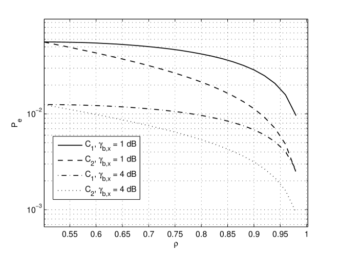
Figure 3: Bit error probability curves in the uncoded case

V Packet error probability evaluation and Optimal convolutional code searching strategy

In this Section, and in the rest of the paper, we consider convolutional coding schemes [23], [24]. Such schemes allow an easy coding implementation with very low power and memory requirements and, hence, they seem to be particularly suitable for utilization in wireless sensors’ networks. Let’s now focus on the evaluation of packet error probability at the decoder in presence of perfect side-information estimation. As in traditional convolutional coding, it is possible to derive an upper bound of the bit error probability as the weighted sum of the pairwise error probabilities relative to all paths which diverge from the zero state and marge again after a certain number of transitions [23]. This is possible because of the linearity of the code and because the pairwise error probability (23) depends only on input and output weights $d_{x}$ and $d_{z}$, and not on the actual transmitted sequence.
In particular, it is possible to evaluate the input-output transfer function $T(W,D)$ by means of the state transition relations over the modified state diagram [23]. The generic form of $T(W,D)$ is:

$$\begin{array}[]{cl}T(W,D)=\sum\limits_{w,d}\beta_{w,d}W^{w}D^{d}\end{array}$$ (26)

where $\beta_{w,d}$ denotes the number of paths that start from the zero state and reemerge with the zero state and that are associated with an input sequence of weight $w$, and an output sequence of weight $d$. Accordingly, we can get an upper bound of the bit error probability of ${\mathbf{x}}$ as:

$$\begin{array}[]{cl}{P}_{b,x}\leq\sum\limits_{w,d}\beta_{w,d}^{(x)}\times w\times{P}_{e}\left(d,w,\gamma_{b,x}\right)\end{array}$$ (27)

where $\beta_{w,d}^{(x)}$ is the $\beta_{w,d}$ term for the first encoder’s code and $P_{e}(d,w,\gamma_{b,x})$ is the pairwise error probability (23) for $d_{z}=d$ and $d_{x}=w$. On account of the symmetry of the problem (7), the union bound of the bit error probability of ${\mathbf{y}}$ is:

$$\begin{array}[]{cl}{P}_{b,y}\leq\sum\limits_{w,d}\beta_{w,d}^{(y)}\times w\times{P}_{e}\left(d,w,\gamma_{b,y}\right)\end{array}$$ (28)

where $\beta_{w,d}^{(y)}$ is the $\beta_{w,d}$ term for the second encoder’s code and $\gamma_{b,y}=\frac{\xi_{b,y}}{N_{0}}$.
Following a similar procedure, it is then possible to derive the packet error probabilities. To this aim, let’s start by denoting to as $L_{pkt}$ the packet data length and let’s assume that $L_{pkt}$ is much higher than the constraint lengths of the codes (the assumption is reasonable for the low complexity convolutional codes that are considered in this paper). In this case, since the first-error events which contribute with non negligible terms to the summations (27) and (28) have a length of few times the code’s constraint length, we can assume that the number of first-error events in a packet is equal to $L_{pkt}$ . Hence, the upper bounds ${P}_{d,x}$ and ${P}_{d,y}$ of the packet error rate can be easily derived as:

$$\begin{array}[]{cl}{P}_{d,x}\leq\sum\limits_{w,d}\beta_{w,d}^{(x)}\times L_{pkt}\times{P}_{e}\left(d,w,\gamma_{b,x}\right)\\ {P}_{d,y}\leq\sum\limits_{w,d}\beta_{w,d}^{(y)}\times L_{pkt}\times{P}_{e}\left(d,w,\gamma_{b,y}\right)\end{array}$$ (29)

Basing on the procedure derived above, it is now possible to implement an exhaustive search over all possible codes’ structures with the aim of finding the optimum code, intended as the code which minimizes the average packet error rate upper bound ${P}_{d}=\frac{{P}_{d,x}+{P}_{d,y}}{2}$. We will assume in the following that sensor 1 and sensor 2 use the same code, and that $k=1$ and $n=2$. In this situation, a code is univocally determined by the generator polynomials $G^{(1)}(D)=g^{(1)}_{\nu}\times D^{\nu}+g^{(1)}_{\nu-1}D^{\nu-1}+g^{(1)}_{\nu-2}D^{\nu-2}+\ldots+g^{(1)}_{1}D^{1}+g^{(1)}_{0}$, $G^{(2)}(D)=g^{(2)}_{\nu}\times D^{\nu}+g^{(2)}_{\nu-1}D^{\nu-1}+g^{(2)}_{\nu-2}D^{\nu-2}+\ldots+g^{(2)}_{1}D^{1}+g^{(2)}_{0}$ and by the feedback polynomial $H(D)=h_{\nu}\times D^{\nu}+h_{\nu-1}D^{\nu-1}+h_{\nu-2}D^{\nu-2}+\ldots+h_{1}D^{1}+h_{0}$, where $\nu$ is the number of shift registers of the code (i.e., the number of states is $2^{\nu}$) and $g^{(1)}_{k}=\left\{0,1\right\}$, $g^{(2)}_{k}=\left\{0,1\right\}$, $h_{k}=\left\{0,1\right\}$. Hence, the exhaustive search is performed by considering all possible polynomials, i.e., all $2^{3(\nu+1)}$ possible values of $G^{(1)}(D)$, $G^{(2)}(D)$, and $H(D)$. It is worth noting that when $H(D)=0$ the code is non-recursive while when $H(D)\neq 0$ the code becomes recursive. Table I shows the optimum code’s structure obtained by exhaustive search for $\gamma_{b,x}=\gamma_{b,y}=3$ dB and for $\nu=3$. Three different values of $\rho$, i.e., $\rho=0.8$, $\rho=0.9$ and $\rho=0.95$, has been considered and three different codes, namely $C_{80}$, $C_{90}$ and $C_{95}$, have been correspondingly obtained.

	$C_{80}$ : $p=0.8$	$C_{90}$ : $p=0.9$	$C_{95}$ : $p=0.95$
$G^{(1)}(D)$	$D^{3}+D^{2}+1$	$D^{3}+D+1$	$D^{3}+D+1$
$G^{(2)}(D)$	$D^{3}+D^{2}+D+1$	$D^{3}+D^{2}+D+1$	$D^{3}+D^{2}+1$
$H(D)$	$D^{3}+D+1$	$D^{3}+D^{2}+1$	$D^{3}+D^{2}+D+1$

$\mathbf{Table~{}I}$: Generator polynomials of the optimum codes

As it is evident from previous Sections’ analysis, the optimum code structure depends on the signal to noise ratios, i.e., different values of $\gamma_{b,x}$ and $\gamma_{b,y}$ lead to different optimum codes. However, by running the optimum code searching algorithm for a set of different signal to noise ratios, we have verified that the optimum code’s structure remain the same over a wide range of $\gamma_{b,x}$ and $\gamma_{b,y}$ and, hence, we can tentatively state that $C_{80}$, $C_{90}$ and $C_{95}$ are the optimum codes for $\nu$ = 3 and for $\rho=0.8$, $\rho=0.9$ and $\rho=0.95$.

VI Results and comparisons

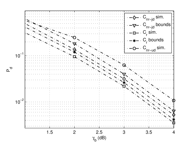
Figure 4: Simulations results and theoretical bounds for $\rho=0.8$ and $L_{pkt}=100$

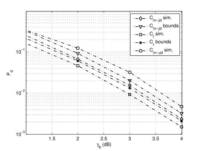
Figure 5: Simulations results and theoretical bounds for $\rho=0.8$ and $L_{pkt}=50$

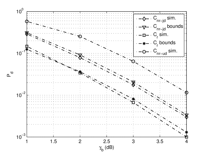
Figure 6: Simulations results and theoretical bounds for $\rho=0.9$ and $L_{pkt}=100$

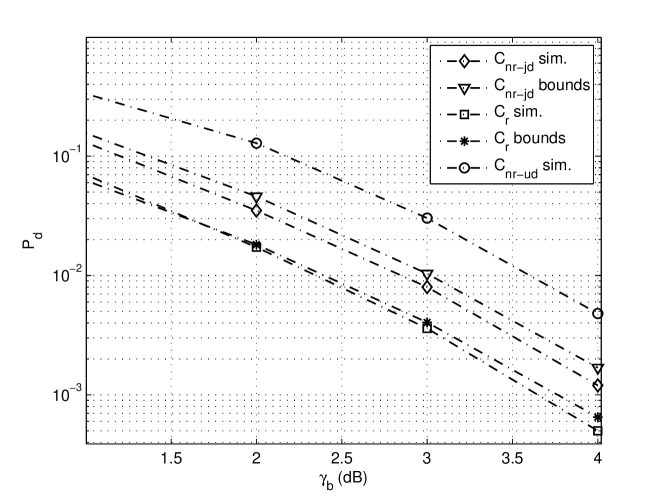
Figure 7: Simulations results and theoretical bounds for $\rho=0.9$ and $L_{pkt}=50$

In order to test the effectiveness of the code searching strategy shown in Section IV, computer simulations of the scenario proposed in this paper have been carried out and comparisons with the theoretical error bounds have been derived as well. In the simulated scenario, channel decoding is based on the iterative approach described in Section V.
The results are shown in Figs. 4-7. In particular, in Fig. 4 and 5 we set $\rho=0.8$ while in Fig. 6 and 7 we set $\rho=0.9$. Besides, a packet length $L_{pkt}=100$ is considered in Figs. 4 and 6, while a packet length $L_{pkt}=50$ is considered in Figs. 5 and 7. In the legend, sim. indicates simulation results and bounds indicates theoretical bounds. Different values of $\gamma_{b,x}=\gamma_{b,y}$ have been considered in all Figs. and indicated in the abscissa as $\gamma_{b}$. In the ordinate we have plotted the average packet error probability ${P}_{d}=\frac{{P}_{d,x}+{P}_{d,y}}{2}$. In these Figures we show results for the optimum recursive codes reported in Table I, referred to as $C_{r}$, and for the $G^{(1)}(D)=D^{3}+D^{2}+1$, $G^{(2)}(D)=D^{3}+D^{2}+D+1$ non-recursive code which is optimum in the uncorrelated scenario [24]. Results obtained for the non-recursive code has been derived for both the joint detection and the unjoint detection case, and are referred to as $C_{nr-jd}$ and $C_{nr-ud}$, respectively . Unjoint detection means that the intrinsic correlation among information signals is not taken into account at the receivers and detection depicted in Figure 2 is performed in only one step. In this case soft output measures are not necessary and, hence, we use a simple Viterbi decoder with hard output.
Notice that, according to the analysis discussed in the previous Sections, the theoretical error bounds are expected to represent packet error probability’s upper bounds (e.g., union bound probabilities). As a matter of fact, the theoretical bounds actually represent packet error probability’s upper bounds for low packet error rates, when the assumption $\rho^{\prime}=\rho$ is reasonable (13). Instead, for high packet error rates, i.e., for low $\gamma_{b}$, the theoretical bounds tend in some cases to superimpose the simulation curves. This is because for high bit error rates, i.e., for high packet error rates, the side-information is affected by non negligible errors and the hypothesis of perfect side information made in the analysis is not valid anymore. However, the theoretical bounds represent in all cases a good approximation of the simulation results.
By observing again Figs. 4-7, the following conclusions can be drawn. The optimum recursive codes allows to get an actual performance gain with respect to the non-recursive scheme, thus confirming the validity of the theoretical analysis described in previous Sections. Such a performance gain is particularly evident for high $\rho$ values, e.g., the performance gain at $P_{d}=0.01$ is nearly of $0.6$ dB for $\rho=0.9$ while for $\rho=0.8$ the gain is less then $0.3$ dB. Comparisons with the unjoint detection case show that, as expected, joint detection allows to get a noticeable performance gain with respect to the unjoint case (from $0.6$ dB for $\rho=0.8$ to more than $1.3$ dB for $\rho=0.9$).
In order to assess the validity of the joint source-channel coding approach considered in this paper, let’s now provide a comparison with a transmitting scheme which performs distributed source coding achieving the Slepian-Wolf compression limit, and independent convolutional channel coding. Note that such a scheme is ideal, since the Slepian-Wolf compression limit cannot be achieved with practical source coding schemes. For comparison purposes, we focus on the $\rho=0.9393$ case and we start by observing that the ideal compression limit is equal to the joint entropy of the two information signals $H({\mathbf{x}},{\mathbf{y}})$ = $H({\mathbf{x}})$ + $H({\mathbf{x}}|{\mathbf{y}})$ = $1-\rho\times log_{2}(\rho)-(1-\rho)\times log_{2}(1-\rho)$ = $1.33$. In order to get a fair comparison, let’s now assume that the transmitter with ideal Slepian Wolf compressor, referred to as $SW$ in the following, has at its disposal the same total energy and the same transmitting time as the joint source-channel coding transmitter without source compression proposed in this paper, referred to as $JS-CC$ in the following. This means that the $SW$ transmitters can use the same energies $\xi_{x}$ and $\xi_{y}$ as the $JS-CC$ transmitters and a reduced channel coding rates $r_{sw}=\frac{1.33}{2}\times r=2/3r$, $r$ being the channel coding rate for $JS-CC$. To be more specific, considering again $r=1/2$ for the $JS-CC$ case, the $SW$ transmitting scheme can be modeled as two independent transmitters which have to deliver $L_{pkt,sw}=2/3L_{pkt}$ independent information bits each one , using a channel rate $r_{sw}=1/3$ and transmitting energies $\xi_{x}$ and $\xi_{y}$. As for the $JS-CC$ transmitting scheme, we consider both the recursive $C_{95}$ channel coding scheme shown in Table I and the $r=1/2$ non-recursive coding scheme described above. As before, the two cases are referred to as $C_{r}$ and $C_{nr-jd}$, respectively. Note that in both cases we perform the iterative joint decoding scheme described in the previous Section in an attempt to exploit the correlation between information signals. Instead, since distributed compression fully eliminates the correlation between information signals, in the $SW$ case unjoint detection with hard Viterbi decoding is performed at the receiver. As for the channel coding scheme, we consider in the $SW$ case a non-recursive 1/3 convolutional code with $\nu=3$ and with generator polynomials $G^{(2)}(D)=D^{3}+D+1$, $G^{(2)}(D)=D^{3}+D^{2}+1$, $G^{(3)}(D)=D^{3}+D^{2}+D+1$, [24].
In order to provide an extensive set of comparisons between $C_{r}$, $C_{nr-jd}$ and $SW$ we consider a more general channel model than the AWGN considered so far. In particular, we assume that the link gains $\alpha_{x}$ and $\alpha_{y}$ are RICE distributed [24] with RICE factor $K_{R}$ equal to $0$ (i.e., Rayleigh case), $10$, and $\infty$ (i.e., AWGN case). The three cases are shown in Figs. 8, 9 and 10, respectively. We consider in all cases a packet length $L_{pkt}=100$. Moreover, we assume that the two transmitters use the same transmitting energy per coded sample $\xi=\xi_{x}=\xi_{y}$. In the abscissa we show the average received power $E({\xi}_{rx})=E\left(|\alpha_{x}|^{2}\right)\times\xi_{x}=E\left(|\alpha_{y}|^{2}\right)\times\xi_{y}$ expressed in dB. Note that the average $\gamma_{b}$ terms can be straightforwardly derived as $E({\gamma}_{b})=\frac{E({\xi}_{rx})}{2r}=E({\xi}_{rx})$ for the $C_{r}$ and $C_{nr-jd}$ cases, and $E({\gamma}_{b})=\frac{E({\xi}_{rx})}{2r_{sw}}=1.5\times E({\xi}_{rx})$ for the $SW$ case. It is worth noting that the comparisons shown in Figs. 8, 9 and 10 are fair in that $C_{r}$, $C_{nr-jd}$ and $SW$ use the same global energy to transmit the same amount of information bits in the same delivering time.
Notice from Fig. 8 that in the AWGN case $SW$ works better than the other two schemes, even if the optimum recursive scheme $C_{r}$ allows to reduce the gap from more then one dB to a fraction of dB. The most interesting and, dare we say, surprising results are shown in Figs. 9 and 10 where the $C_{r}$ decoding scheme clearly outperform $SW$ with a gain of more then 1 dB in the Rayleigh case and of almost 1 dB in the Rice case, while $C_{nr-jd}$ and $SW$ perform almost the same. This result confirms that, in presence of many-to-one transmissions, separation between source and channel coding is not optimum. The rationale for this result is mainly because in presence of an unbalanced signal quality from the two transmitters (e.g., independent fading), leaving a correlation between the two information signals can be helpful since the better quality received signal can be used as side information for detecting the other signal. In other words, the proposed joint decoding scheme allows to get a diversity gain which is not obtainable by the $SW$ scheme. Such a diversity gain is due to the inherent correlation between information signals and, hence, can be exploited at the receiver without implementing any kind of cooperation between the transmitters.

VII Conclusions

A simple wireless sensor networks scenario, where two nodes detect correlated sources and deliver them to a central collector via a wireless link, has been considered. In this scenario, a joint source-channel coding scheme based on low-complexity convolutional codes has been presented. Similarly to turbo or LDPC schemes, the complexity at the decoder has been kept low thanks to the use of an iterative joint decoding scheme, where the output of each decoder is fed to the other decoder’s input as a-priori information. For the proposed convolutional coding/decoding scheme we have derived a novel analytical framework for evaluating an upper bound of joint-detection packet error probability and for deriving the optimum coding scheme, i.e., the code which minimizes the packet error probability. Comparisons with simulation results show that the proposed analytical framework is effective. In particular, in the AWGN case the optimum recursive coding scheme derived from the analysis allows to clearly outperform classical non-recursive schemes. As for the fading scenario, the proposed transmitting scheme allows to get a diversity gain which is not obtainable by the classical Slepian-Wolf approach to distributed source coding of correlated sources. Such a diversity gain allows the proposed scheme to clearly outperform a Slepian-Wolf scheme based on ideal compression of distributed sources.

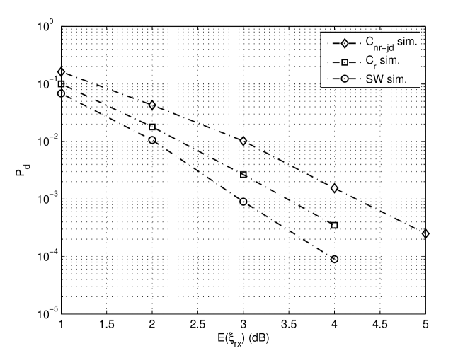
Figure 8: Comparison with the SW case: AWGN channel

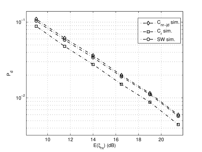
Figure 9: Comparison with the SW case: Rayleigh channel model

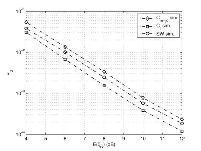
Figure 10: Comparison with the SW case: Rice channel model with $K_{R}=10$

References

- [1] I. F. Akyildiz, W. Su, Y. Sankasubramaniam, and E. Cayirci ”Wireless Sensor Networks: A Survey,” Computer Networks Vol. 38, pp. 393-422, 2002
- [2] J. Barros and S. Servetto ”On the capacity of the reachback channel in wireless sensor networks,” IEEE Workshop on Multimedia Signal Processing, pp. 408-411, 2002.
- [3] P. Gupta and P. Kumar ”The capacity of wireless networks,” IEEE Transactions on Information Theory 46, March 2000
- [4] H. E. Gamal ”On the scaling laws of dense wireless sensor networks,” IEEE Transactions on Information Theory April 2003
- [5] A. Aaron and B. Girod ”Compression with side information using turbo codes,” Proc. IEEE Data Compression Conference Snowbird, Utah, Apr. 2002
- [6] J. Bajcsy and P. Mitran ”Coding for the Slepian-Wolf problem with turbo codes,” Proc. IEEE Proc. Global Telecommu. Conf. Nov. 2001
- [7] I. Deslauriers and J. Bajcsy ”Serial Turbo Coding for Data Compression and the Slepian-Wolf Problem,” Proc. Information Theory Workshop Mar. 2003
- [8] Z. Xiong, A. D. Liveris, and S. Cheng ”Distributed source coding for sensor networks,” IEEE Signal Process. Mag., Sep. 2004
- [9] Andrej Stefanov and Elza Erkip, ”Cooperative Coding for Wireless Networks,” IEEE Transactions on Communications, vol. 52, No. 9, pp. 1470-1476, September 2004.
- [10] Andrej Stefanov and Elza Erkip, ”Cooperative Space-Time Coding for Wireless Networks,” IEEE Transactions on Communications, vol. 53, No. 11, pp. 1804-1809, November 2005.
- [11] A. Sendonaris, E. Erkip and B. Aazhang, ”User cooperation diversity-Part I: System description,” IEEE Transactions on Communications, vol. 51, no. 11, pp. 1927-1938, November 2003.
- [12] A. Sendonaris, E. Erkip and B. Aazhang, ”User cooperation diversity-Part II: Implementation aspects and performance analysis,” IEEE Transactions on Communications, vol. 51, no. 11, pp. 1927-1938, November 2003.
- [13] Laneman, J.N.; Wornell, G.W., ”Distributed space-time-coded protocols for exploiting cooperative diversity in wireless networks,” IEEE Transactions on Information Theory, vol. 51, no. 11, pp. 1939-1948, November 2003.
- [14] Laneman, J.N.; Tse, D.N.C.; Wornell, G.W., ”Cooperative diversity in wireless networks: Efficient protocols and outage behavior,” IEEE Transactions on Information Theory, Volume 50, Issue 12, Dec. 2004 Page(s):3062 - 3080
- [15] Murugan, A.D. Gopala, P.K. Gamal, H.E., ”Correlated sources over wireless channels: cooperative source-channel coding,” Selected Areas in Communications, IEEE Journal on, Aug. 2004 Volume: 22, Issue: 6 On page(s): 988- 998
- [16] J. Garcia-Frias and Y. Zhao ”Compression of correlated binary sources using turbo codes,” IEEE. Communications Letters vol. 5, no. 10, pp. 417-419, October 2001
- [17] F. Daneshgaran, M. Laddomada, M. Mondin, ”Iterative Joint Channel Decoding of Correlated Sources Employing Serially Concatenated Convolutional Codes,” Information Theory, IEEE Transaction on, Aug. 2005 Volume: 51, Issue: 7
- [18] J. Maramatsu, T. Uyematsu, T. Wadayama, ”Low-density Parity-Check Matrices for Coding of Correlated Sources,” Information Theory, IEEE Transaction on, October 2005 Volume: 51, Issue: 10
- [19] F. Daneshgaran, M. Laddomada, M. Mondin, ”LDPC-Based Channel Coding of Correlated Sourcesn With Iterative Joint Decoding,” Communications, IEEE Transaction on, April. 2006 Volume: 54, Issue: 4
- [20] J. Lassing, E. Str m, T. Ottosson, ”Packet Error Rates of Terminated and Tailbiting Convolutional Codes,” T. Wysocki, M. Darnell, B. Honary, editors, Advanced Signal Processing for Communication Systems, The Kluwer International Series in Engineering and Computer Science, Vol.703, Boston, Sep 2002.
- [21] J. Hagenauer, ”Source-Controlled Channel Decoding,” Communications, IEEE Transaction on, Vol.43, No. 9, Sep. 1995.
- [22] F. Dabeshgaran, M. Laddomada, M. Mondin, ”Iterative Joint Channel Decoding of Correlated Sources,” Wireless Communications, IEEE Transactions on, October 2006 Volume: 5, Issue: 10
- [23] B Sklar, ”Digital Communications: Fundamentals and Applications,” New Jersey, Prentice Hall, 2001
- [24] John G. Proakis ”Digital Communications,” Singapore: Mc Graw-Hill, 1995.