Scaling theory put into practice: first-principles modeling of transport in doped silicon nanowires

Abstract

We combine the ideas of scaling theory and universal conductance fluctuations with density-functional theory to analyze the conductance properties of doped silicon nanowires. Specifically, we study the cross-over from ballistic to diffusive transport in boron (B) or phosphorus (P) doped Si-nanowires by computing the mean free path, sample averaged conductance $\langle G\rangle$, and sample-to-sample variations std$(G)$ as a function of energy, doping density, wire length, and the radial dopant profile. Our main findings are: (i) the main trends can be predicted quantitatively based on the scattering properties of single dopants; (ii) the sample-to-sample fluctuations depend on energy but not on doping density, thereby displaying a degree of universality, and (iii) in the diffusive regime the analytical predictions of the DMPK theory are in good agreement with our ab initio calculations.

Silicon nanowires (SiNWs) are strong candidates for future nanoelectronic and sensor applications Cui and Lieber (2001); Cui et al. (2003); Patolsky and Lieber (2005). In most of the demonstrated devices the SiNWs are either $p-$ or $n-$doped during the fabrication process. Very thin SiNWs with diameters below 5 nm have been synthesized by several groups Ma et al. (2003); Holmes et al. (2000); Wu et al. (2004), and due to the small cross section, scattering by dopants is likely to be very important. Moreover, due to reduced acoustic phonon scattering in quasi one-dimensional systems, long coherence lengths might be possible even at room temperature Lu et al. (2005), thus emphasizing the importance of defect scattering. At the same time sample-to-sample variations become a crucial issue: when the device length and the mean free path are comparable, and shorter than the coherence length, variations of the positions of the individual dopant atoms can affect the conductance of the wire significantly.

The mathematical theory of the conductance of disordered quasi one-dimensional systems has reached a high level of understanding in the diffusive as well as the localization regime Lee and Ramakrishnan (1985); Beenakker (1997). A standard way to model disorder, analytically as well as numerically, is to introduce random noise (Anderson disorder), which in a tight-binding description is included through randomly varying on-site energies. It does not seem obvious that a random disorder is an adequate description of real physical disorder, such as dopants or vacancies, nor is there any obvious connection between a physical defect density and the amplitude of the random disorder. In particular, if only a few dopants are present in a wire, the system is in the crossover region from ballistic to diffusive transport and the discrete and local nature of the impurities must be modeled adequately.

Several recent theoretical works considered dopants in SiNWs using density-functional theory (DFT) Fernandez-Serra et al. (2006); Peelaers et al. (2006); Singh et al. (2006), mainly focusing on the structural and energetic properties of different radial dopant positions. As an important first step towards the modeling of physical SiNWs, Fernandez-Serra et al. Fernandez-Serra et al. (2006) considered the scattering properties of single P dopants in thin nanowires.

In this Letter we complete the analysis by calculating the conductance of long nanowires with a random distribution of dopants (either P or B) along the wire. We calculate the sample averaged conductance $\langle G\rangle$, elastic mean free path (MFP) $l_{e}$, localization length $\xi$, and the sample-to-sample fluctuations characterized by the sample standard deviation std($G$). We show that all these quantities can be understood and accurately estimated from the scattering properties of the single dopants, implying that relatively simple calculations are sufficient in practical device modeling. The sample-to-sample fluctuations at a given energy and dopant type vary with $L/l_{e}$ in a universal way independently on the dopant concentration, and in the diffusive regime for wire length $l_{e}<L<\xi$, we observe good agreement with analytical predictions of the Dorokhov-Mello-Pereyra-Kumar (DMPK) theory Mello et al. (1988).

Method: The length and energy dependent conductance of each sample is found using the Landauer formalism together with a standard recursive Green’s function (GF) approach where the full scattering region containing the dopant atoms is constructed by repeatedly adding small unit cells Markussen et al. (2006). The unit cells are constructed using first–principles local orbital DFT calculations Soler et al. (2002); DFT . We emphasize that our combined DFT and GF approach to calculate the conductance is fully ab initio within the low bias coherent transport regime.

\begin{overpic}[width=208.13574pt]{fig1.eps} \put(47.0,27.0){\includegraphics[width=45.52824pt]{fig1inset.eps}} \end{overpic}

Figure 1: (color online). Transmissions through wires with a single B (left) or P (right) dopant atom placed at the different radial positions shown in the inset. Left: energies relative to the valence band maximum, $E_{v}$; Right; energies relative to the conduction band minimum, $E_{c}$. The band gap is $2.84\,$eV.

Single dopants: Figure 1 shows the transmission vs. energy through infinite hydrogen passivated wires containing only a single dopant atom placed at five different substitutional positions (1-5) indicated in the inset. The left part shows the transmission for B dopants at energies in the valence band while the right part shows results for P dopants at energies in the conduction band. We notice that there are special resonant energies where the conductance abruptly drops, similar to those observed in Ref. Fernandez-Serra et al. (2006), due to enhanced local densities of states at the dopant atoms associated with quasi-bound states. As also pointed out in Ref. Fernandez-Serra et al. (2006), there are significant differences in the scattering properties between dopants located in the bulk of the wire and those situated at the surface. Interestingly, there are qualitative differences between P and B dopants. While B in position 1 (middle of wire) is a weak scatterer in the valence band, P at the same position is the strongest scatterer in the conduction band. For thicker wires the majority of the dopants are likely to be bulk-like and our calculations thus predict P-doped wires to have smaller mobilities than B-doped wires with the same dopant concentration, in agreement with experimental results Cui et al. (2000).

Long wires: While the scattering properties of the single dopants are interesting in their own right, real nanowires contain several dopants with a certain distribution along the wire direction as well as in the radial direction. Due to interference effects between successive scattering events, it is not obvious if the single-dopant results carry over to the long wire case. In the rest of this Letter we investigate the conductance of long wires. In particular we examine to what extent the long wire properties, such as mean conductance $\langle G\rangle$ and variations std$(G)$, can be determined from the scattering properties of the single dopants.

A single recursive GF calculation yields the conductance of a SiNW with a given dopant distribution, length and energy. At each energy we do this calculation for 300 different realizations of the dopant positions, and we repeat these calculations for a range of wire lengths, 10 nm $<L<$ 200 nm, all with the same dopant density. The dopants are distributed randomly along the wire direction Ran as well as radially. The sample-averaged resistance increases linearly for wire lengths shorter than the localization length, as shown in the left inset in Fig. 2. The initial linearly increasing resistance defines the energy dependent MFP, $l_{e}(E)$, through the relation $R(L,E)=R_{c}(E)+R_{c}(E)L/l_{e}(E)$ for wire lengths $L<\xi$, where $R_{c}(E)=1/G_{0}(E)=h/(2e^{2}\,N)$ is the contact resistance of a pristine wire with $N$ conducting channels. It has recently been shown that this definition of the MFP agrees with values found using the Kubo formula and Fermi’s golden rule Avriller et al. (2006); Markussen et al. (2006). In the linear resistance region, we suggest that on average, the scattering resistances from the dopants add classically according to Ohm’s law, i.e. the mean resistance of a wire of length $L<\xi$ and average dopant-dopant separation $d$ is given by

$$\langle R(L,E)\rangle=R_{c}(E)+\langle R_{s}(E)\rangle\,L/d.$$ (1)

$\langle R_{s}(E)\rangle$ is the average scattering resistance of the different dopant positions which can be estimated from the single dopant conductances, $G(E)$, in Fig. 1 as $\langle R_{s}(E)\rangle=1/\langle G(E)\rangle-1/G_{0}(E)$. From Eq. (1) we get an estimate of the MFP, $l_{e}^{\prime}=R_{c}\,d/\langle R_{s}\rangle$.

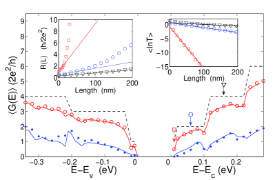
Figure 2: (color online). Energy dependent average conductance calculated at $L=10\,$nm (circles) and $L=100\,$nm (dots) with the GF method. Solid lines follow from Eq. (1). Left inset: Resistance vs. wire length at energies $E-E_{c}=$ 0.01, 0.06 and 0.16 eV (indicated with arrows in the main frame; same behavior is seen in the entire energy range). Solid lines are obtained using Eq. (1). Right inset: $\langle\ln T\rangle$ vs. length at the same energies, where $T=G/(2e^{2}/h)$ is the transmission. Solid lines are linear fits in the interval 150 nm$\,<L<200\,$nm from which the localization length is determined.

Figure 2 shows the sample averaged energy dependent conductance at wire lengths $L=10\,$nm (circles) and $L=100\,$nm (dots) for B and P doped wires with an average dopant-dopant separation $d=10\,$nm (corresponding to a bulk doping density of $n\approx 10^{19}\,$cm^-3) and uniform radial dopant distribution. The dashed line shows the conductance of the pristine wire, while the solid curves are estimated conductances obtained from the single dopant transmissions shown in Fig. 1 using Eq. (1). It is evident that the average conductances are well reproduced by the single-dopant results.

We emphasize that Eq. (1) is only valid in the quasi-ballistice ($L<l_{e}$) and diffusive ($l_{e}<L<\xi$) regimes. In the localization regime ($L>\xi$), the resistance increases exponentially, $R(L)\sim\exp(L/\xi)$. We have calculated the localization length from the $\langle\ln T\rangle$ vs. L curves shown in the right inset of Fig. 2 as $\xi=-1/{\rm slope}$, and the slope is determined from a linear fit in the interval $150\,$nm$<L<200\,$nm. In Table 1 we show the resulting MFPs ($l_{e}$) and localization lengths ($\xi$) at four different energies. These are compared with the estimates $l_{e}^{\prime}=R_{c}\,d/\langle R_{s}\rangle$ based on the single dopant transmissions, and $\xi^{\prime}=l_{e}^{\prime}\,(N+1)/2$ (this relation follows from random matrix theory Beenakker (1997)). It is evident that both the MFP and the localization length can be estimated fairly accurately from the single dopant transmissions with a maximum error of $24\%$. We also note that the ratio $\xi/l_{e}$ agrees with the prediction $(N+1)/2$ with a maximum deviation of $30\%$.

$E-E_{c}$ (eV)	$\;\;N\;\;$	$\;\;l_{e}\;$ (nm)	$\;\;l_{e}^{\prime}\;$ (nm)	$\;\;\xi\;$ (nm)	$\;\;\xi^{\prime}\;$ (nm)
0.01	1	10	8	7	8
0.06	2	37	46	59	56
0.16	4	49	47	133	123
0.26	6	37	37	164	130

Table 1: MFP and localization lengths obtained from sample averaging ($l_{e}$ and $\xi$), and estimated values, $l_{e}^{\prime}$ and $\xi^{\prime}$, obtained from the single dopant transmissions. $N$ is the number of conducting channels.

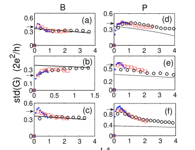
Figure 3: (Color online) Sample standard deviation, std($G$) vs. normalized length $L/l_{e}$ with average dopant-dopant separation $d=19\,$nm (dots), $d=10\,$nm (squares) and $d=5\,$nm (circles). (a)-(c) correspond to the energies $E-E_{v}=-0.12,\;-0.20,\;-0.30\,$eV in the valence band for B doped wires, (d)-(f) correspond to the energies $E-E_{c}=0.06,\;0.16,\;0.26\,$eV in the conduction band for P doped wires. The solid lines are analytical solutions to the DMPK equation of Ref.Mirlin et al. (1994) which equals the UCF value $0.73\,e^{2}/h$ at $L=0$. The small arrows mark the maximum std($G$), $s$, estimated from the single-dopant transmissions.

Sample fluctuations: An interesting question is whether or not the sample-to-sample variations can also be understood in terms of the single-dopant transmissions. In the diffusive regime we expect the variations to be close to the universal conductance fluctuation (UCF) value, $0.73\,e^{2}/h$ for quasi-one dimensional systems Lee and Stone (1985). Figure 3 shows the standard deviation, std($G$), plotted against normalized length, $L/l_{e}$, for B (a)-(c) and P (d)-(f) doped wires. The conductance fluctuations corresponding to different concentrations lie close to each other, and we therefore conclude that at a specific energy and type of dopant, the sample variations are independent of dopant concentration but only depend on the normalized length. This is in accordance with the theory of UCF Lee and Stone (1985) and single parameter scaling theory Abrahams et al. (1979) which predict that the sample fluctuations are independent on the disorder strength. For modeling purposes this is a very convenient result because one can limit the simulations to only one dopant concentration.

In the diffusive limit, $L/l_{e}>1$, analytical results are known for std$(G(L))$. For quasi one-dimensional systems with many conducting channels and weak random disorder, the DMPK equation Mello et al. (1988) predicts a weak length dependence, std$(G(L))=\sqrt{8/15-64/315\cdot L/\xi}\,\cdot e^{2}/h$, Mirlin et al. (1994), shown in Fig. 3 (solid lines). As the length of the wire decreases, the sample fluctuations increase, and in most cases a maximum in std($G$) is reached around $L/l_{e}=0.5$. In the limit $L\rightarrow 0$ there are no dopants in the wire and the sample-to-sample variations vanish.

We next address this maximum value and the general behavior of the sample-to-sample fluctuations vs. $L$ using the single-dopant conductance results. Figure 4(a) shows the maximum values of std($G$) vs. energy for P-doped wires with a uniform radial distribution (squares) and pure surface doping (circles). In the former case all the dopant positions 1-5 are equally probablerad while in the latter the dopants can only be in position 4 or 5, cf. inset in Fig. 1. The lower solid line in Fig.4(a) shows the standard deviation $s=$std($\{G_{0},G_{0},G_{4},G_{5}\}$), where $G_{0}$ is the conductance of a pristine wire while $G_{4}$ and $G_{5}$ are the single-dopant conductances with the P dopant placed at position 4 and 5. This sequence represents a situation where there is 50$\%$ chance for a pristine wire, and 50$\%$ chance for a wire with a single dopant either at position 4 or 5. The upper solid line in Fig. 4(a) shows similar values for the uniform dopant distribution. When $s$ is larger than the UCF value (the horizontal dashed line), the maximum std($G$) clearly follows the trends in $s$. When $s$ is smaller than the UCF value, the maximum std($G$) lies close to the UCF level.

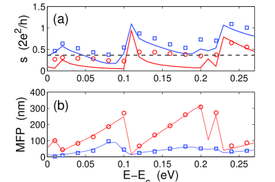
Figure 4: (color online). Maximal standard deviation (a) for for P doped wires ($d=10\,$nm,) with a homogeneous radial distribution (squares) and a pure surface doped wire (circles). The solid lines show the standard deviation, $s$, among the single dopant transmissions and the pristine wire, and the dashed line marks the UCF value $0.73\,e^{2}/h$. Panel (b) shows the MFP vs. energy for the two radial distributions (circles and squares). The lines represent values obtained from the single dopant transmissions.

We conclude that the shape of the std($G$) vs. $L/l_{e}$ curves in Fig. 3 can be qualitatively predicted from the single-dopant transmissions: When $s$, indicated with small arrows in Fig. 3, is smaller than the UCF value ($0.73e^{2}/h$), we expect std($G$) to approach the analytical line from below. The B doped wires in Fig. 3(b) show such a behaviour. Otherwise, if $s$ is larger than the UCF value, std($G$) will reach a maximum value close to $s$ and approach the analytical line from above.

Mean free path: Figure 4(a) shows that the sample fluctuations are significantly reduced in the surface doped wires due to the weaker and more uniform scattering properties of the surface positions. The MFP also depends significantly on the radial distribution as seen in Fig. 4(b), showing the MFP for P doped wires with a uniform (circles) and pure surface (squares) distribution of dopants. The solid lines are estimated from the single-dopant transmissions using Eq. (1) once again showing that the mean values of the conductance can be accurately estimated from the single dopants. A very significant increase in the MFP is observed for the surface doped wires as compared to the uniform distribution. This might suggest that increased device performance could be achieved if the P dopants are located close to the surface, which indeed are the energetically most favorable positions in the wires studied here and also found in Ref. Fernandez-Serra et al. (2006, 2006). There are, however, potential problems with dopants close to the surface, as they can be passivated by addition of an extra hydrogen atom Fernandez-Serra et al. (2006); Singh et al. (2006).

In conclusion, we have considered the conductance properties in B and P doped SiNWs. We find that the sample averaged conductance and the sample-to-sample fluctuations as well as the mean free path and localization length can be predicted quantitatively from the scattering properties of the single dopants. Time consuming sample averaging can thus be avoided, which greatly simplify modelling of the statistical conductance properties. These findings may have a high impact on first-principles modelling of electron transport in nanowires.