On systematic scan for sampling $H$-colourings of the path

Abstract

This paper is concerned with sampling from the uniform distribution on $H$-colourings of the $n$-vertex path using systematic scan Markov chains. An $H$-colouring of the $n$-vertex path is a homomorphism from the $n$-vertex path to some fixed graph $H$. We show that systematic scan for $H$-colourings of the $n$-vertex path mixes in $O(\log n)$ scans for any fixed $H$. This is a significant improvement over the previous bound on the mixing time which was $O(n^{5})$ scans. Furthermore we show that for a slightly more restricted family of $H$ (where any two vertices are connected by a 2-edge path) systematic scan also mixes in $O(\log n)$ scans for any scan order. Finally, for completeness, we show that a random update Markov chain mixes in $O(n\log n)$ updates for any fixed $H$, improving the previous bound on the mixing time from $O(n^{5})$ updates.

1 Introduction

Many combinatorial problems are of interest to computer scientists both in their own right and due to their natural applications to statistical physics. Such problems can often be studied by considering homomorphisms from the graph of interest $G$ to some fixed graph $H$. This is known as an $H$-colouring of $G$. The vertices of $H$ correspond to colours and the edges of $H$ specify which colours are allowed to be adjacent in an $H$-colouring of a graph. Let $H=(C,E)$ by any fixed graph. We will refer to $C$ as the set of colours (in the literature it is often referred to as the set of spins). Formally an $H$-colouring of a graph $G=(V,E_{G})$ is a function $h:V\rightarrow C$ such that $(h(v),h(u))\in E$ for all edges $(v,u)\in E_{G}$ of $G$. For example if $H$ is the graph in Figure 1 then $C=\{a,b\}$ and sites (in order to be consistent with existing literature, e.g. Weitz [28], we will refer to elements of $V$ as sites throughout this paper) assigned colour $a$ in an $H$-colouring of $G$ are permitted to be adjacent to sites assigned both $a$ and $b$, but sites assigned colour $b$ can only be adjacent to sites assigned colour $a$.

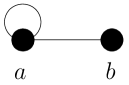
Figure 1: The graph describing the independent sets model. Sites assigned colour $a$ are “out” and sites assigned $b$ are “in”.

Due to the applicability of $H$-colourings to models in statistical physics, and for ease of analysis, $H$-colouring problems are often studied by restricting attention to a specific graph $H$. We now give a few examples of special cases of $H$ that correspond to important $H$-colouring problems. $H$-colourings using the graph $H$ from Figure 1 correspond to independent set configurations of a graph where sites assigned colour $a$ are “out” and sites assigned $b$ are “in” the independent set. It is usual to assign weight $1$ to vertex $a$ and some positive weight $\lambda>0$ to vertex $b$ in $H$. Independent sets (also known as the hard-core lattice gas model when using the weighted setting) is one of the most commonly studied type of $H$-colourings in theoretical computer science. Another well-studied case is when $H$ is the $q$-clique, in which case $H$-colourings correspond to proper $q$-colourings of the underlying graph. A proper $q$-colouring is a configuration where no two adjacent sites are permitted to be assigned the same colour. It is worth noting that proper $q$-colourings correspond to the $q$-state anti-ferromagnetic Potts model at zero temperature which is a well-studied model in statistical physics. Other well-known examples include the Beach model introduced by Burton and Steif [6] and the $q$-particle Widom-Rowlinson due to Widom and Rowlinson [30]. The graph corresponding to the Beach model is shown in Figure 2. The Beach model was originally introduced as an example of a physical system, with underlying graph $\mathbb{Z}^{d}$, which exhibits more than a single measure of maximal entropy when $d>1$. The $q$-particle Widom-Rowlinson model is a model of gas consisting of $q$ types of particles that are not allowed to be adjacent to each other. The graph corresponding to the $q=4$ case is shown in Figure 3 where the center vertex represents empty sites and each remaining vertex represents a particle.

Figure 2: The graph describing the Beach model.

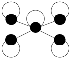
Figure 3: The graph describing the 4-particle Widom-Rowlinson model.

The problem of determining whether a graph has an $H$-colouring for a specific $H$ has been well-studied and Hell and Nešetřil [20] gave a complete characterisation of graphs $H$ for which this problem is NP-complete. In particular, they showed that if $H$ has a loop or is bipartite then the problem is in P, and that the problem is NP-complete for any other fixed $H$. A complete dichotomy is also known for the problem of counting the number of $H$-colourings. This is due to Dyer and Greenhill [15] who showed that if $H$ has at least one so-called nontrivial component then the counting problem is is #P-complete. Otherwise it is in P. A trivial component is a connected component which is either a complete graph with all loops present, or a complete bipartite graph with no loops present. They furthermore showed that the same dichotomy holds even when the underlying graph is of bounded degree, which is significant since in many physical applications the underlying graph tends to be of low degree. Interestingly the above characterisation for the decision problem does not hold for bounded degree graphs as shown by Galluccio, Hell and Nešetřil [17]. Despite the hardness of exactly counting the number of $H$-colourings it remains possible to approximately count the number of $H$-colourings of a graph as long as it is possible to sample efficiently from the (near) uniform distribution of $H$-colourings. This is due to a general counting-to-sampling reduction of Dyer, Goldberg and Jerrum [12] that holds for any fixed $H$ and any underlying graph.

Sampling from the uniform distribution of $H$-colourings of a graph, which for this discussion we will denote by $\pi$, is a challenging task and some results about the complexity thereof are known. Goldberg, Kelk and Paterson [18] have shown that, if $H$ has no nontrivial components, then the sampling problem is intractable in a complexity-theoretic sense. That is, they prove that there is unlikely to be any Polynomial Almost Uniform Sampler for $H$-colourings by reducing the problem of sampling from the (near) uniform distribution of $H$-colourings to the problem of counting independent sets in bipartite graphs, which in turn is complete for a logically-defined subclass of #P (see Dyer, Goldberg, Greenhill and Jerrum [11] for results about this complexity class). This does, however, not rule out the possibility of sampling from the uniform distribution of $H$-colourings of more restricted graphs, such as the $n$-vertex path, as we will be focusing on in this paper. This sampling task may be carried out by simulating some suitable random dynamics converging to $\pi$. Ensuring that a dynamics converges to $\pi$ is generally straightforward, but obtaining good upper bounds on the number of steps required for the dynamics to become sufficiently close to $\pi$ is a much more difficult problem. Due to a lack of theoretical convergence results, scientists conducting experiments by simulating such dynamics are at times forced to “guess” (using some heuristic methods) the number of steps required for their dynamics to be sufficiently close to the desired distribution. See for example Cowles and Carlin [8] for a comprehensive review of some diagnostic tools used to empirically determine these convergence rates. By establishing rigorous bounds on the convergence rates (mixing time) of these dynamics computer scientists can provide underpinnings for this type of experimental work and also allow a more structured approach to be taken.

Analysing the mixing time of Markov chains for $H$-colouring problems is a well-studied area in theoretical computer science. There is a substantial body of literature concerned with inventing Markov chains for sampling from the uniform distribution of $H$-colourings of graphs and providing bounds on their mixing times. When an $H$-colouring corresponds to a proper $q$-colouring of graph with maximum vertex-degree $\Delta$ then Jerrum [21], and independently Salas and Sokal [26], showed that a simple Markov chain mixes in $O(n\log n)$ updates when $q>2\Delta$. This Markov chain makes transitions by selecting a site $v$ and a colour $c$ uniformly at random, and then recolouring site $v$ to $c$ if doing so results in a proper $q$-colouring of the graph. By considering a more complicated Markov chain Vigoda [27] was able to weaken the restriction on $q$ to $q>(11/6)\Delta$ colours being sufficient for proving mixing in $O(n\log n)$ updates. This remains the least number of colours required for mixing of a Markov chain on general graphs, however the number of colours can be further reduced for special graphs. For example, when the underlying graph is the square grid then Goldberg, Martin and Paterson [19] gave a hand-proof that $q=7$ colours are sufficient for mixing in $O(n\log n)$ updates by proving a condition called “strong spacial mixing”. Achlioptas, Molloy, Moore and van Bussel [1] showed that $q=6$ colours are sufficient for a Markov chain for proper colourings of the grid to mix in $O(n\log n)$ updates using a computational proof. As a final example for proper $q$-colourings Martinelli, Sinclair and Weitz [24] showed that $q=\Delta+2$ colours are sufficient for $O(n\log n)$ mixing when the underlying graph is a tree, improving a similar result by Kenyon, Mossel and Peres [22]. When $H$ correspond to independent set configurations of a graph with parameter $\lambda$ (that is, the vertex labeled $b$ in Figure 1 is assigned some positive weight $\lambda$ and $a$ has weight 1) then $\lambda<\frac{2}{\Delta-2}$ is sufficient for $O(n\log n)$ mixing as shown by Dyer and Greenhill [16] and independently Luby and Vigoda [23] (although the latter result is restricted to triangle-free graphs). When $\Delta\leq 4$ these results include the $\lambda=1$ case which is of special interest to computer scientists since it corresponds to sampling from the uniform distribution on independent sets of the graph. Weitz [29] has recently improved the condition on $\lambda$ to $\lambda<(\Delta-1)^{\Delta-1}/(\Delta-2)^{\Delta}$ which notably includes the $\lambda=1$ case for $\Delta=5$. When $\Delta\geq 6$ and $\lambda=1$ then Dyer, Frieze and Jerrum [10] have shown that there exists a bipartite graph $G_{0}$ such that any so-called cautious Markov chain on independent set configurations of $G_{0}$ has (at least) exponential mixing time (in the number of sites of $G_{0}$). A Markov chain is said to be cautious if it is only allowed to change the state of a constant number of sites at the time. This negative result was generalised to $H$-colourings by Cooper, Dyer and Frieze [7]. Their result applies to graphs $H$ that are either bipartite or have at least one loop present, and is not a complete graph with all loops present (observe that for such an $H$ the decision problem is in P and the counting problem is in #P as discussed above). In particular this result guarantees the existence of a $\Delta$-regular graph $G_{0}$ (with $\Delta$ depending on $H$) such that any cautious Markov chain on the set of $H$-colourings of $G_{0}$, and with uniform stationary distribution, has a mixing time that is at least exponential in the number of sites of $G_{0}$.

While much is now understood about the mixing times of Markov chains, the types of Markov chains frequently studied by computer scientists fall under a family of Markov chains that we call random update Markov chains. We say that a Markov chain on the set of $H$-colourings of a graph is a random update Markov chain when one step of the the process consists of randomly selecting a set of sites (often a single site) and updating the colours assigned to those sites according to some well-defined distribution induced by $\pi$. The mixing time of a random update Markov chain is measured in the number of updates required in order for the Markov chain to be sufficiently close to $\pi$. We point out that all the positive results described above are for random update Markov chains. An alternative to random update Markov chains is to construct a Markov chain that cycles through and updates the sites (or subsets of sites) in a deterministic order. We call this a systematic scan Markov chain (or systematic scan for short). Systematic scan may be more intuitively appealing in terms of implementation, however until recently this type of dynamics has largely resisted analysis when applied to $H$-colouring problems. Perhaps some of the first analyses of systematic scan were due to Amit [3] and Diaconis and Ram [9] who respectively studied systematic scan in the context of sampling from multivariate Gaussian distributions and generating random elements of a finite group. The mixing time of a systematic scan Markov chain is measured in the number of scans of the graph required to be sufficiently close to $\pi$ and throughout this paper it holds that one scan takes $O(n)$ updates where $n$ is the number of sites of the graph. It is important to note that systematic scan remains a random process since the method used to update the colour assigned to the selected set of sites is a randomised procedure drawing from some well-defined distribution induced by $\pi$. This paper is concerned with sampling from the uniform distribution of $H$-colourings of the $n$-vertex path using systematic scan Markov chains.

Only few results providing bounds on the mixing time of systematic scan Markov chains for sampling from the uniform distribution of $H$-colourings exist in the literature and almost all of them focus on proper $q$-colourings of bounded degree graphs. For general graphs systematic scan is known to mix in $O(\log n)$ scans whenever $q\geq 2\Delta$, where $\Delta$ is the maximum vertex-degree of the graph, by updating both end-points of an edge in each move. This is due to a recent result by Pedersen [25] which improves the polynomial in the $q=2\Delta$ case from a result of Dyer, Goldberg and Jerrum [13] that is obtained by updating one site at the time. If the underlying graph is bipartite then a systematic scan mixes in $O(\log n)$ scans whenever $q>f(\Delta)$ where $f(\Delta)\to\beta\Delta$ as $\Delta\to\infty$ and $\beta\approx 1.76$. This result is obtained by a careful construction of the metric used in the coupling construction and is due to Bordewich, Dyer and Karpinski [4]. Furthermore, Dyer, Goldberg and Jerrum [14] have shown that a systematic scan for proper $3$-colourings of the $n$-vertex path mixes in $\Theta(n^{2}\log n)$ scans when considering a systematic scan which updates a single site at the time using the Metropolis update rule. In the same paper it is also shown that systematic scan for $H$-colourings of the $n$-vertex path mixes in $O(n^{5})$ scans for any fixed $H$ and that a random update Markov chain for $H$-colourings of the $n$-vertex path mixes in $O(n^{5})$ updates. The authors suggest, however, that both of these bounds are unlikely to be tight and we will significantly improve them both in this paper.

In this paper we prove that systematic scan for $H$-colourings of the $n$-vertex path mixes in $O(\log n)$ scans for any fixed graph $H$, by updating a constant-size block of sites at each step. By constant-size we mean that the number of sites contained in a block is bounded independently of $n$. We do however allow the block-sizes to depend on $H$ (since $H$ is a fixed graph). We will present two different Markov chains in order to achieve this aim. In Section 2 we show that if $H$ is a graph in which any pair of colours are connected by a 2-edge path then a systematic scan mixes for any order of a set of blocks, provided that the blocks are large enough. We will use a recent result by Pedersen [25], which is based on a technique known as Dobrushin uniqueness, in order to establish the mixing time of this Markov chain. In Section 3 we extend this result to all connected graphs $H$, although at the expense of imposing a specific order on the scan. The proof of mixing uses path coupling [5] in this case. Finally, for completeness, we give a proof that a random update Markov chain for $H$-colourings of the $n$-vertex path mixes in $O(n\log n)$ updates for any fixed graph $H$. This result is presented in Section 4.

1.1 Preliminaries and statement of results

Consider a fixed (and connected) graph $H=(C,E)$ with maximum vertex-degree $\Delta_{H}$. Let $C=\{1,\dots,q\}$ be referred to as the set of colours. Also let $V=\{1,\ldots,n\}$ be the set of sites of the $n$-vertex path and in particular let $V_{1}$ be the set of sites with odd indices and $V_{2}$ the set of sites with even indices. We formally say that an $H$-colouring of the $n$-vertex path is a function $h$ from $V$ to $C$ such that $(h(i),h(i+1))\in E$ for all $i\in V\setminus\{n\}$. Let $\Omega^{+}$ be the set of all configurations (all possible assignments of colours to the sites) of the $n$-vertex path and $\Omega$ be the set of all $H$-colourings of the $n$-vertex path for the given $H$. Define $\pi$ to be the uniform distribution on $\Omega$. If $x\in\Omega^{+}$ is a configuration and $j\in V$ is a site then $x_{j}$ denotes the colour assigned to $j$ in configuration $x$ and for any set $\Lambda\subseteq V$ let $x_{\Lambda}=\bigcup_{v\in\Lambda}\{x_{v}\}$ be the set of colours assigned to sites in $\Lambda$. For colours $c,d\in C$ and an integer $l$ let $D_{c,d}^{(l)}$ be the uniform distribution on $H$-colourings of the region of consecutive sites $L=\{v_{1},\dots,v_{l}\}\subset V$ consistent with site $v_{1}$ being adjacent to a site $i\in V\setminus L$ assigned colour $c$ and site $v_{l}$ being adjacent to a site in $V\setminus L$ assigned colour $d$. Also let $D_{c,d}^{(l)}(v_{j})$ be the distribution on the colour assigned to site $v_{j}$ induced by $D_{c,d}^{(l)}$. Observe that for $s<l$

$$\left[D_{c,d}^{(l)}\mid v_{1}=c_{1},\dots,v_{s}=c_{s}\right]=D_{c_{s},d}^{(l-s)}$$

where $D_{c,d}^{(l)}\mid v_{1}=c_{1},\dots,v_{s}=c_{s}$ is the uniform distribution on $H$-colourings of $L$ conditioned on site $v_{1}$ being assigned colour $c_{1}$, $v_{2}$ colour $c_{2}$ and so on until $v_{s}$ being assigned colour $c_{s}$.

Let $\mathcal{M}$ be any ergodic Markov chain with state space $\Omega$ and transition matrix $P$. By classical theory (see e.g. Aldous [2]) $\mathcal{M}$ has a unique stationary distribution, which we will denote $\pi$. The mixing time from an initial configuration $x\in\Omega$ is the number of steps, that is applications of $P$, required for $\mathcal{M}$ to become sufficiently close to $\pi$. Formally the mixing time of $\mathcal{M}$ from an initial configuration $x\in\Omega$ is defined, as a function of the deviation $\varepsilon$ from stationarity, by

$$\textnormal{Mix}_{x}(\mathcal{M},\varepsilon)=\min\{t>0\;:\;\mathrm{d}_{\mathrm{TV}}(P^{t}(x,\cdot),\pi)\leq\varepsilon\},$$

where

$$\mathrm{d}_{\mathrm{TV}}(\theta_{1},\theta_{2})=\frac{1}{2}\sum_{i}|\theta_{1}(i)-\theta_{2}(i)|=\max_{A\subseteq\Omega^{+}}|\theta_{1}(A)-\theta_{2}(A)|$$

is the total variation distance between two distributions $\theta_{1}$ and $\theta_{2}$ on $\Omega$. The mixing time $\textnormal{Mix}(M,\varepsilon)$ of $\mathcal{M}$ is then obtained by maximising over all possible initial configurations

$$\textnormal{Mix}(\mathcal{M},\varepsilon)=\max_{x\in\Omega}\textnormal{Mix}_{x}(\mathcal{M},\varepsilon).$$

We say that $\mathcal{M}$ is rapidly mixing if the mixing time of $\mathcal{M}$ is polynomial in $n$ and $\log(\varepsilon^{-1})$.

We study Markov chains that perform heat-bath moves on a constant number of sites at the time. For any configuration $x\in\Omega^{+}$ and subset of sites $\Lambda\subseteq V$ we let $\Omega_{\Lambda}(x)$ be the set of configurations where the colours assigned to the endpoints of each edge containing a site in $\Lambda$ are also adjacent in $H$. A heat-bath move on $\Lambda$ starting from configuration $x$ is performed by drawing a new configuration from the uniform distribution on $\Omega_{\Lambda}(x)$. We would normally let $\Omega$ be the state space of our Markov chains, however, if $H$ is bipartite then we encounter a minor technical difficulty because the Markov chain may not be ergodic. We overcome this ergodicity issue by partitioning the state space as follows. If $C_{1}$ and $C_{2}$ are the colour classes of $H$ then $\Omega_{1}=\{x\in\Omega:x_{1}\in C_{1}\}$ is the set of $H$-colourings where the first site of the path is assigned a colour from $C_{1}$. Observe that in fact each site in $V_{1}$ is assigned a colour from $C_{1}$ and each site in $V_{2}$ is assigned a colour from $C_{2}$. Similarly $\Omega_{2}=\{x\in\Omega:x_{1}\in C_{1}\}$ is the set of $H$-colourings where the first site is assigned a colour from $C_{2}$. Intuitively, $\Omega_{1}$ and $\Omega_{2}$ are the two connected components of $\Omega$ and we will show (Lemma 17) that the constructed Markov chains are ergodic on either $\Omega_{1}$ or $\Omega_{2}$. To see that $\Omega_{1}\cup\Omega_{2}$ contain all $H$-colourings of the $n$-vertex path it is enough to observe that if $x\in\Omega$ then any pair of adjacent sites of the $n$-vertex path must be assigned colours from opposite colour classes of $H$ in $x$. We let $\Omega_{\sim}$ be the relevant state space of the Markov chains in order to ensure ergodicity. In particular, if $H$ is non-bipartite then $\Omega_{\sim}=\Omega$. Otherwise $H$ is bipartite and we let $\Omega_{\sim}$ be one of $\Omega_{1}$ and $\Omega_{2}$. This is the same partition used by Dyer et al. in [14]. See also Cooper et al. [7] for a discussion of this issue in the context of $H$-colourings.

We are now ready to formally define the systematic scan Markov chains we will study in this paper and state our theorems. Let $l_{1}=\lceil\Delta_{H}^{2}\log(\Delta_{H}^{2}+1)\rceil+1$. Then let $\{\Theta_{1},\dots,\Theta_{m_{1}}\}$ be any set of $m_{1}=\lceil n/l_{1}\rceil$ blocks where each block consists of $l_{1}$ consecutive sites and $\bigcup_{k=1}^{m_{1}}\Theta_{k}=V$. For each block $\Theta_{k}$ we define $P^{[k]}$ to be the transition matrix on the state space $\Omega_{\sim}$ for performing a heat-bath move on $\Theta_{k}$.

Definition 1.

For any integer $n$ we let $\mathcal{M}_{\textnormal{AnyOrder}}$ be the systematic scan Markov chain, on the state space $\Omega_{\sim}$, with transition matrix $\Pi_{k=1}^{m_{1}}P^{[k]}$.

It is worth pointing out that the following result holds for any order of the blocks, as is the case for all results obtained by Dobrushin uniqueness (see e.g. Dyer et al [13]). In Section 2 we will use a recent result by Pedersen [25] to prove the following theorem.

Theorem 2.

Let $H$ be a fixed connected graph and consider the systematic scan Markov chain $\mathcal{M}_{\textnormal{AnyOrder}}$ on the state space $\Omega_{\sim}$. Suppose that $H$ is a graph in which every two sites are connected by a $2$-edge path. Then mixing time of $\mathcal{M}_{\textnormal{AnyOrder}}$ is

$$\textnormal{Mix}(\mathcal{M}_{\textnormal{AnyOrder}},\varepsilon)\leq\Delta_{H}^{2}(\Delta_{H}^{2}+1)\log(n\varepsilon^{-1})$$

scans of the $n$-vertex path. This corresponds to $O(n\log n)$ updates by the construction of the set of blocks.

Remark.

Note that that each $H$ for which Theorem 2 is valid is non-bipartite so $\Omega_{\sim}=\Omega$.

Remark.

Several well known graphs satisfy the condition of Theorem 2, for example Widom-Rowlinson configurations, independent set configurations and proper $q$-colourings for $q\geq 3$. The fact that an $H$ corresponding to 3-colourings satisfies the condition of the theorem is particularly interesting since a lower bound of $\Omega(n^{2}\log n)$ scans for single site systematic scan on the path is proved in Dyer at al. [14]. This means that using a simple single site coupling cannot be sufficient to establishing Theorem 2 for any family of $H$ including 3-colourings and hence we have to use block updates.

While many natural $H$-colouring problems belong to the family covered by Theorem 2, others (e.g. Beach configurations) are not included. We go on to show that systematic scan mixes in $O(\log n)$ scans for any fixed graph $H$ by placing more strict restrictions on the construction of the blocks and the order of the scan. Let $s=4q+1$, $\beta=\lceil\log(2sq^{s}+1)\rceil q^{s}$ and $l_{2}=2\beta s$. For any integer $n$ consider the following set of $m_{2}+1=\lfloor 2n/l_{2}\rfloor$ blocks $\{\Theta_{0},\dots,\Theta_{m_{2}}\}$ where

$$\Theta_{k}=\{k\beta s+1,\dots,\min((k+2)\beta s,n)\}.$$

We observe that $\bigcup_{k=0}^{m_{2}}\Theta_{k}=V$ by construction of the set of blocks. Furthermore note that the size of $\Theta_{m_{2}}$ is at least $\beta s$ and that the size of every other block is $l_{2}$.

Definition 3.

For any integer $n$ we let $\mathcal{M}_{\textnormal{FixedOrder}}$ be the systematic scan Markov chain, on the state space $\Omega_{\sim}$, which performs a heat-bath move on each block in the order $\Theta_{0},\dots,\Theta_{m_{2}}$.

In Section 3 we will use path coupling [5] to prove the following theorem, which improves the mixing time from the corresponding result in Dyer et al. [14] from $O(n^{5})$ scans to $O(\log n)$ scans.

Theorem 4.

Let $H$ be any fixed connected graph and consider the systematic scan Markov chain $\mathcal{M}_{\textnormal{FixedOrder}}$ on the state space $\Omega_{\sim}$. The mixing time of $\mathcal{M}_{\textnormal{FixedOrder}}$ is

$$\textnormal{Mix}(\mathcal{M}_{\textnormal{FixedOrder}},\varepsilon)\leq(4sq^{s}+2)\log(n\varepsilon^{-1})$$

scans of the $n$-vertex path. This corresponds to $O(n\log n)$ updates by the construction of the set of blocks.

Remark.

It is worth remarking at this point that Theorem 4 eclipses Theorem 2 in the sense that it shows the existence of a systematic scan for a broader family of $H$ than Theorem 2 but with the same (asymptotic) mixing time. The result stated as Theorem 2 however remains interesting in its own right since it applies to any order of the scan. Following the proof of Theorem 2 we will discuss (Observation 14) the obstacles one encounters when attempting to extend Theorem 2 to a larger family of $H$ using the same method of proof.

For completeness we finally consider a random update Markov chain for $H$-colourings of the $n$-vertex path. Let $\gamma=2q^{s}+1$ and define the following set of $n+s\gamma-1$ blocks, which is constructed such that each site is contained in exactly $s\gamma$ blocks

$$\Theta_{k}=\begin{cases}\{k,\dots,\min(k+s\gamma-1,n)\}&\textnormal{when }k\in\{1,\dots,n\}\\ \{1,\dots,n+s\gamma-k\}&\textnormal{when }k\in\{n+1,\dots,n+s\gamma-1\}.\end{cases}$$

Definition 5.

For any integer $n$ we let $\mathcal{M}_{\textnormal{RND}}$ be the random update Markov chain, on the state space $\Omega_{\sim}$, which at each step selects a block uniformly at random and performs a heat-bath move on it.

In Section 4 we will use path coupling [5] to prove the following theorem, which improves the mixing time from the corresponding result in Dyer et al. [14] from $O(n^{5})$ updates to $O(n\log n)$ updates.

Theorem 6.

Let $H$ be any fixed connected graph and consider the random update Markov chain $\mathcal{M}_{\textnormal{RND}}$ on the state space $\Omega_{\sim}$. The mixing time of $\mathcal{M}_{\textnormal{RND}}$ is

$$\textnormal{Mix}(\mathcal{M}_{\textnormal{RND}},\varepsilon)\leq\frac{(n+2sq^{s}+s-1)\log(n\varepsilon^{-1})}{s}$$

block-updates. This corresponds to $O(n\log n)$ updates since the size of each block is at most $s\gamma=O(1)$.

1.2 Review of proof techniques

We now briefly introduce the techniques we will use to bound the mixing time of the above Markov chains. For technical reasons we extend the state space of the Markov chains as follows. Let $\Omega_{1}^{+}$ be the set of configurations where each site in $V_{1}$ is assigned a colour from $C_{1}$ and each site in $V_{2}$ is assigned a colour from $C_{2}$ (recall that $C_{1}$ and $C_{2}$ are the colour classes of $H$). Similarly, $\Omega_{2}^{+}$ is the set of configurations where each site in $V_{1}$ is assigned a colour from $C_{2}$ and each site in $V_{2}$ is assigned a colour from $C_{1}$. Formally

$$\Omega_{1}^{+}=\{x\in\Omega^{+}:x_{V_{1}}\subseteq C_{1},x_{V_{2}}\subseteq C_{2}\}$$

and

$$\Omega_{2}^{+}=\{x\in\Omega^{+}:x_{V_{1}}\subseteq C_{2},x_{V_{2}}\subseteq C_{1}\}.$$

We then extend the state space of the Markov chains to $\Omega_{\sim}^{+}$ where $\Omega_{\sim}^{+}=\Omega^{+}$ if $H$ is not bipartite and $\Omega_{\sim}^{+}$ is one of $\Omega_{1}^{+}$ or $\Omega_{2}^{+}$ when $H$ is bipartite. The extended Markov chains make the same transitions as the original Markov chains on configurations in $\Omega_{\sim}$ and hence the extended chains do not make transitions from configurations in $\Omega_{\sim}$ to configurations outside $\Omega_{\sim}$. The stationary distributions of the extended chains are uniform over the configurations in $\Omega_{\sim}$ and zero elsewhere. This approach is standard and the mixing times of the original chains are bounded above by the mixing time of corresponding chain on the extended state space.

For each site $j\in V$, let $S_{j}$ denote the set of pairs $(x,y)\in\Omega_{\sim}^{+}\times\Omega_{\sim}^{+}$ of configurations that only differ on the colour assigned to site $j$, that is $x_{i}=y_{i}$ for all $i\neq j$. Also let $S=\bigcup_{j\in V}S_{j}$ be the set of all such pairs of configurations.

1.2.1 Dobrushin uniqueness

We will make use of a recent result by Pedersen [25] to prove Theorem 2 by bounding the influence on a site. For completeness we now summarise this result and at the same time point out how the construction of $\mathcal{M}_{\textnormal{AnyOrder}}$ ensures that all required properties are satisfied. First note from the remark after Theorem 2 that each $H$ that we consider is not bipartite and so $\Omega_{\sim}^{+}=\Omega^{+}$. Suppose that $\{\Theta_{1},\dots,\Theta_{m}\}\subseteq V$ is a set of $m$ blocks such that $\bigcup_{k=1}^{m}\Theta_{k}=V$ and that each block $\Theta_{k}$ is associated with a transition matrix $P^{[k]}$ on the state space $\Omega^{+}$. For any configuration $x\in\Omega^{+}$, $P^{[k]}(x,\cdot)$ denotes the distribution on configurations obtained from applying $P^{[k]}$ to $x$. Recall from the definition of $\mathcal{M}_{\textnormal{AnyOrder}}$ that the set of blocks covers $V$ as required and that each transition matrix $P^{[k]}$ represents performing a heat-bath move on $\Theta_{k}$. It is furthermore required that each transition matrix $P^{[k]}$ satisfies the following two properties.

1. If $P^{[k]}(x,y)>0$ then $x_{i}=y_{i}$ for each $i\in V\setminus\Theta_{k}$, and

2. the distribution $\pi$ on $\Omega^{+}$ is invariant with respect to $P^{[k]}.$

Pedersen [25] points out that if $P^{[k]}$ is the transition matrix performing a heat-bath move on $\Theta_{k}$ and $\pi$ is the uniform distribution on $\Omega$, as they both are in the case of $\mathcal{M}_{\textnormal{AnyOrder}}$, then both of these properties are satisfied. These properties ensure that the stationary distribution of any systematic scan Markov chain with transition matrix $\Pi_{k=1}^{m}P^{[k]}$ is $\pi$.

We are now ready to define the parameter $\alpha$ denoting the influence on a site. For any pair of configurations $(x,y)\in S_{i}$ let $\Psi_{k}(x,y)$ be a coupling of the distributions $P^{[k]}(x,\cdot)$ and $P^{[k]}(y,\cdot)$. We remind the reader that a coupling of two distributions $\pi_{1}$ and $\pi_{2}$ on state space $\Omega^{+}$ is a joint distribution on $\Omega^{+}\times\Omega^{+}$ such that the marginal distributions are $\pi_{1}$ and $\pi_{2}$. We let $(x^{\prime},y^{\prime})\in\Psi_{k}(x,y)$ denote that the pair of configurations $(x^{\prime},y^{\prime})$ is drawn from the coupling $\Psi_{k}(x,y)$. We then let

$$\rho_{i,j}^{k}=\max_{(x,y)\in S_{i}}\textnormal{Pr}_{(x^{\prime},y^{\prime})\in\Psi_{k}(x,y)}(x_{j}^{\prime}\neq y_{j}^{\prime})$$

be the influence of site $i$ on site $j$ under $\Theta_{k}$. The influence of $i$ on $j$ is thus the probability that site $j\in\Theta_{k}$ is assigned a different colour in a pair of configurations drawn from the coupling $\Psi_{k}(x,y)$ where $x$ and $y$ differ only on the colour of site $i$. Finally the parameter $\alpha$ denoting the influence on any site is defined as

$$\alpha=\max_{k}\max_{j\in\Theta_{k}}\sum_{i}\rho_{i,j}^{k}.$$

Remark.

Pedersen [25] actually defines $\alpha$ with a positive weight assigned to each site of the graph, however as we will not use the weights in our proof they are omitted from the above definition.

The following theorem bounds the mixing time of a systematic scan Markov chain $\mathcal{M}_{\rightarrow}$ with transition matrix $\Pi_{k=1}^{m}P^{[k]}$. It is worth pointing out that, since the proof makes use of Dobrushin uniqueness, this upper-bound on the mixing time holds for any order of the blocks.

Theorem 7 (Theorem 2, Pedersen [25]).

If $\alpha<1$ then the mixing time of $\mathcal{M}_{\rightarrow}$ satisfies

$$\textnormal{Mix}(\mathcal{M}_{\rightarrow},\varepsilon)\leq\frac{\log(n\varepsilon^{-1})}{1-\alpha}.$$

1.2.2 Path coupling

In order to prove Theorems 4 and 6 we will make use of path coupling [5] which is a well-known, and by now standard, technique for proving rapid mixing of Markov chains. The key idea of path coupling is to define a coupling for pairs of adjacent configurations where the set of all adjacent configurations connects the state space. We will say that a pair of configurations $x,y\in\Omega_{\sim}^{+}$ are adjacent if $(x,y)\in S$. The path coupling machinery then extends the coupling to all pairs of configurations in the state space. For completeness we show that $S$ connects the state space $\Omega_{\sim}^{+}$.

Lemma 8.

The transitive closure of $S$ is the whole of $\Omega_{\sim}^{+}\times\Omega_{\sim}^{+}$.

Proof.

Recall that $S=\bigcup_{i\in V}S_{j}$ where $S_{j}\subseteq\Omega_{\sim}^{+}\times\Omega_{\sim}^{+}$ is the set of pairs $(x,y)\in\Omega_{\sim}^{+}\times\Omega_{\sim}^{+}$ of configurations that differ only on the colour assigned to site $j$. To establish the lemma it is sufficient to, for any pair of configurations $(x,y)\in\Omega_{\sim}^{+}\times\Omega_{\sim}^{+}$, to construct a path $x=z^{0},z^{1},\dots,z^{n}=y$ such that $(z^{j-1},z^{j})\in S_{j}$ for each $j\in\{1,\dots,n\}$. We define $z^{j}$ for $j\in\{1,\dots,n\}$ as follows

$$z_{i}^{j}=\begin{cases}y_{i}&\textnormal{for }1\leq i\leq j\\ x_{i}&\textnormal{for }j<i\leq n.\end{cases}$$

Informally, configuration $z^{j}$ agrees with configuration $y$ from site $1$ to $j$ and with configuration $x$ from site $j+1$ to $n$.

By definition of the configurations $z^{0},\dots,n^{n}$ it follows that $z^{j-1}$ and $z^{j}$ only differ on the colour assigned to site $j$ for each $j\in\{1,\dots,n\}$. Hence we only need to check that $z^{j}\in\Omega_{\sim}^{+}$ for each $j$. If $H$ is non-bipartite then $\Omega_{\sim}^{+}=\Omega^{+}$ so $z^{j}\in\Omega_{\sim}^{+}$ for each $j\in\{1,\dots,n\}$. If $H$ is bipartite then $\Omega_{\sim}^{+}$ is one of $\Omega_{1}^{+}$ or $\Omega_{2}^{+}$. Suppose without loss of generality that $\Omega_{\sim}^{+}=\Omega_{1}^{+}$. Then for each $j\in\{1,\dots n\}$ it holds by definition of $\Omega_{1}^{+}$ that the colours $x_{j}$ and $y_{j}$ must be from the same colour class of $H$ and hence have $z^{j}\in\Omega_{1}^{+}$. ∎

Finally note that $\textnormal{Ham}(x,y)=1$ for any $(x,y)\in S$ where $\textnormal{Ham}(x,y)$ denotes the Hamming distance between configurations $x$ and $y$. The following theorem is sufficient for our needs in this paper, and it is a special case of the general path coupling theorem proved by Bubley and Dyer [5].

Theorem 9 (Bubley, Dyer [5]).

For all pairs $(x,y)\in S$ define a coupling $(x,y)\mapsto(x^{\prime},y^{\prime})$ of a Markov chain $\mathcal{M}$ on the state space $\Omega_{\sim}^{+}$. Suppose that there exists a constant $0<\gamma<1$ such that $\textnormal{{E}}\left[\textnormal{Ham}(x^{\prime},y^{\prime})\right]\leq(1-\gamma)$ for all pairs $(x,y)\in S$. Then the mixing time of $\mathcal{M}$ satisfies

$$\textnormal{Mix}(\mathcal{M},\varepsilon)\leq\frac{\log(n\varepsilon^{-1})}{\gamma}.$$

2 $H$-colourings on the path for a restricted family of $H$

Recall that $\Delta_{H}$ denotes the maximum vertex-degree of some fixed graph $H$ and that $l_{1}=\lceil\Delta_{H}^{2}\log(\Delta_{H}^{2}+1)\rceil+1$. The systematic scan Markov chain $\mathcal{M}_{\textnormal{AnyOrder}}$ on $\Omega_{\sim}$ has transition matrix $\Pi_{k=1}^{m_{1}}P^{[k]}$ where $P^{[k]}$ is the transition matrix for performing a heat-bath move on block $\Theta_{k}$ from a set of $m_{1}=\lceil n/l_{1}\rceil$ size $l_{1}$ blocks covering the $n$-vertex path. We will prove Theorem 2, namely that $\mathcal{M}_{\textnormal{AnyOrder}}$ mixes in $O(\log n)$ scans when $H$ is a graph in which any two colours are connected via a 2-edge path. We will bound the mixing time of $\mathcal{M}_{\textnormal{AnyOrder}}$ by bounding the influence on a site and begin by establishing some lemmas required to construct the coupling needed in the proof of Theorem 2.

Lemma 10.

Suppose that for any $c_{1},c_{2}\in C$ there is a 2-edge path in $H$ from $c_{1}$ to $c_{2}$. Then for any $c_{1},c_{2},d\in C$ and integer $s^{\prime}\geq 2$ there exists a coupling $\psi(D_{c_{1},d}^{(s^{\prime})},D_{c_{2},d}^{(s^{\prime})})$ of $D_{c_{1},d}^{(s^{\prime})}$ and $D_{c_{2},d}^{(s^{\prime})}$ such that

1. $\textnormal{Pr}_{(x^{\prime},y^{\prime})\in\psi(D_{c_{1},d}^{(s^{\prime})},D_{c_{2},d}^{(s^{\prime})})}(x_{v_{1}}^{\prime}\neq y_{v_{1}}^{\prime})\leq 1-\frac{1}{\Delta_{H}^{2}}$ and

2. $\textnormal{Pr}_{(x^{\prime},y^{\prime})\in\psi(D_{c_{1},d}^{(2)},D_{c_{2},d}^{(2)})}(x_{v_{2}}^{\prime}\neq y_{v_{2}}^{\prime})\leq 1-\frac{1}{\Delta_{H}^{2}}.$

Proof.

By the condition of the lemma there exists some $c^{\prime}\in C$ adjacent to both $c_{1}$ and $c_{2}$ in $H$. We prove the statement by considering two cases on $s$.

First suppose that $s^{\prime}=2$. By the condition of the lemma there is some colour $d^{\prime}$ adjacent to both $c^{\prime}$ and $d$ in $H$. There are at most $\Delta_{H}^{2}$ valid $H$-colourings of the sites $v_{1},v_{2}$ in either of the distributions $D_{c_{1},d}^{(2)}$ and $D_{c_{2},d}^{(2)}$, and hence the colouring $h$, which assigns $c^{\prime}$ to $v_{1}$ and $d^{\prime}$ to $v_{2}$, has weight at least $1/\Delta_{H}^{2}$ in both. We construct a coupling $\psi(D_{c_{1},d}^{(2)},D_{c_{2},d}^{(2)})$ such that

$$\textnormal{Pr}_{(x^{\prime},y^{\prime})\in\psi(D_{c_{1},d}^{(2)},D_{c_{2},d}^{(2)})}(x^{\prime}=y^{\prime}=h)\geq\frac{1}{\Delta_{H}^{2}}.$$

The rest of the coupling is arbitrary. This gives the following bounds on the disagreement probabilities at $v_{1}$ and $v_{2}$

$$\textnormal{Pr}_{(x^{\prime},y^{\prime})\in\psi(D_{c_{1},d}^{(2)},D_{c_{2},d}^{(2)})}(x_{v_{1}}^{\prime}=y_{v_{1}}^{\prime})\geq\textnormal{Pr}_{(x^{\prime},y^{\prime})\in\psi(D_{c_{1},d}^{(2)},D_{c_{2},d}^{(2)})}(x_{v_{1}}^{\prime}=y_{v_{1}}^{\prime}=c^{\prime})\geq\frac{1}{\Delta_{H}^{2}}$$

which establishes $(i)$ for $s^{\prime}=2$ and

$$\textnormal{Pr}_{(x^{\prime},y^{\prime})\in\psi(D_{c_{1},d}^{(2)},D_{c_{2},d}^{(2)})}(x_{v_{2}}^{\prime}=y_{v_{2}}^{\prime})\geq\textnormal{Pr}_{(x^{\prime},y^{\prime})\in\psi(D_{c_{1},d}^{(2)},D_{c_{2},d}^{(2)})}(x_{v_{2}}^{\prime}=y_{v_{2}}^{\prime}=d^{\prime})\geq\frac{1}{\Delta_{H}^{2}}$$

which establishes $(ii)$.

Now suppose $s^{\prime}>2$. Let $adj(c)$ denote the set of colours adjacent to $c$ in $H$ and $n_{k}$ the number of $H$-colourings on the sites $v_{4},\dots,v_{s^{\prime}}$ consistent with $v_{3}$ being assigned colour $k\in C$ and $v_{s^{\prime}}$ being adjacent to a site (out side the block) coloured $d$. Also let $p_{c,k}$ be the number of $H$-colourings of $v_{1},v_{2},v_{3}$ assigning colour $c$ to $v_{1}$ and $k$ to $v_{3}$ without regard to other sites. Finally let $z_{i}$ be the number of $H$-colourings with positive measure in $D_{c_{i},d}^{(s^{\prime})}$ and assume without loss of generality that $z_{1}\geq z_{2}$.

There are at most $\Delta_{H}$ colours available for each site in the block which gives $p_{c,k}\leq\Delta_{H}$ for any $c,k\in C$ and hence

$$z_{1}=\sum_{c\in adj(c_{1})}\sum_{k\in C}p_{c,k}n_{k}\leq\Delta_{H}\sum_{c\in adj(c_{1})}\sum_{k\in C}n_{k}\leq\Delta_{H}^{2}\sum_{k\in C}n_{k}.$$

Now let $H(c^{\prime})$ be the set of all $H$-colourings with positive measure in $D_{c_{1},d}^{(s^{\prime})}$ that assign colour $c^{\prime}$ to site $v_{1}$. Let $h(c^{\prime})$ denote the size of this set. Now $p_{c,k}\geq 1$ for any $c,k\in C$ since there is a 2-edge path in $H$ between any two colours and hence

$$h(c^{\prime})=\sum_{k\in C}p_{c^{\prime},k}n_{k}\geq\sum_{k\in C}n_{k}.$$

Observe that, for any $h\in H(c^{\prime})$, $h$ is at least as likely in $D_{c_{2},d}^{(s^{\prime})}$ as in $D_{c_{1},d}^{(s^{\prime})}$ since we have assumed $z_{1}\geq z_{2}$ without loss of generality. We construct a coupling $\psi(D_{c_{1},d}^{(s^{\prime})},D_{c_{2},d}^{(s^{\prime})})$ of $D_{c_{1},d}^{(s^{\prime})}$ and $D_{c_{2},d}^{(s^{\prime})}$ in which for each $h\in H(c^{\prime})$

$$\textnormal{Pr}_{(x^{\prime},y^{\prime})\in\psi(D_{c_{1},d}^{(s^{\prime})},D_{c_{2},d}^{(s^{\prime})})}(x^{\prime}=y^{\prime}=h)\geq\frac{1}{z_{1}}.$$

The rest of the coupling is arbitrary. Hence

$$\textnormal{Pr}_{(x^{\prime},y^{\prime})\in\psi(D_{c_{1},d}^{(s^{\prime})},D_{c_{2},d}^{(s^{\prime})})}(x_{v_{1}}^{\prime}=y_{v_{1}}^{\prime}) \geq\sum_{h\in H(c^{\prime})}\textnormal{Pr}_{(x^{\prime},y^{\prime})\in\psi(D_{c_{1},d}^{(s^{\prime})},D_{c_{2},d}^{(s^{\prime})})}(x^{\prime}=y^{\prime}=h)$$

$$\geq\frac{h(c^{\prime})}{z_{1}}$$

$$\geq\frac{1}{\Delta_{H}^{2}}$$

using the bounds on $z_{1}$ and $h(c^{\prime})$. This completes the proof. ∎

We then use Lemma 10 to bound the disagreement probabilities at each site of of the block when a pair of configurations are drawn from a recursively constructed coupling.

Lemma 11.

Suppose that for any $c_{1},c_{2}\in C$ there is a 2-edge path in $H$ from $c_{1}$ to $c_{2}$. Then for all $c_{1},c_{2},d\in C$ and integers $l^{\prime}\geq 2$ there exists a coupling $\Psi(D_{c_{1},d}^{(l^{\prime})},D_{c_{2},d}^{(l^{\prime})})$ of $D_{c_{1},d}^{(l^{\prime})}$ and $D_{c_{2},d}^{(l^{\prime})}$ in which for $j\in\{1,\dots,l^{\prime}-1\}$

$$\textnormal{Pr}_{(x^{\prime},y^{\prime})\in\Psi(D_{c_{1},d}^{(l^{\prime})},D_{c_{2},d}^{(l^{\prime})})}(x_{v_{j}}^{\prime}\neq y_{v_{j}}^{\prime})\leq\left(1-\frac{1}{\Delta_{H}^{2}}\right)^{j}$$

and

$$\textnormal{Pr}_{(x^{\prime},y^{\prime})\in\Psi(D_{c_{1},d}^{(l^{\prime})},D_{c_{2},d}^{(l^{\prime})})}(x_{v_{l}}^{\prime}\neq y_{v_{l}}^{\prime})\leq\left(1-\frac{1}{\Delta_{H}^{2}}\right)^{l^{\prime}-1}.$$

Proof.

We recursively construct a coupling $\Psi(D_{c_{1},d}^{(l^{\prime})},D_{c_{2},d}^{(l^{\prime})})$ of $D_{c_{1},d}^{(l^{\prime})}$ and $D_{c_{2},d}^{(l^{\prime})}$ using the method set out in Goldberg et al. [19] as follows. Firstly $l^{\prime}=2$ is the base case and we use the coupling from Lemma 10. For $l^{\prime}\geq 3$ we construct a coupling using the following two step process.

1. Couple $D_{c_{1},d}^{(l^{\prime})}(v_{1})$ and $D_{c_{2},d}^{(l^{\prime})}(v_{1})$ greedily to maximise the probability of assigning the same colour to site $v_{1}$ in both distributions.

2. If the same colour $c$ was chosen for $v_{1}$ in both distributions in step 1 then the set of valid $H$-colourings of the remaining sites are the same in both distributions. Hence the conditional distributions $D_{c_{1},d}^{(l^{\prime})}\mid v_{1}=c$ and $D_{c_{2},d}^{(l^{\prime})}\mid v_{1}=c$ are the same and the rest of the coupling is trivial. Otherwise, for all pairs $(c_{1}^{\prime},c_{2}^{\prime})$ of distinct colours recursively couple $D_{c_{1},d}^{(l^{\prime})}\mid v_{1}=c_{1}^{\prime}=D_{c_{1}^{\prime},d}^{(l^{\prime}-1)}$ and $D_{c_{2},d}^{(l^{\prime})}\mid v_{1}=c_{2}^{\prime}=D_{c_{2}^{\prime},d}^{(l^{\prime}-1)}$ which is a sub problem of size $l^{\prime}-1$.

This completes the coupling construction.

Now for $j\in\{1,\dots,l^{\prime}-1\}$ we prove by induction that

$$\textnormal{Pr}_{(x^{\prime},y^{\prime})\in\Psi(D_{c_{1},d}^{(l^{\prime})},D_{c_{2},d}^{(l^{\prime})})}(x_{v_{j}}^{\prime}\neq y_{v_{j}}^{\prime})\leq\left(1-\frac{1}{\Delta_{H}^{2}}\right)^{j}.$$ (1)

The base case, $j=1$, follows from Lemma 10 since we couple the colour at site $v_{1}$ greedily to maximise the probability of agreement at $v_{1}$ in the first step of the recursive coupling. Now suppose that (1) is true for $j-1$ then

Pr $${}_{(x^{\prime},y^{\prime})\in\Psi(D_{c_{1},d}^{(l^{\prime})},D_{c_{2},d}^{(l^{\prime})})}(x_{v_{j}}^{\prime}\neq y_{v_{j}}^{\prime})$$

$$=\sum_{c_{1}^{\prime},c_{2}^{\prime}}\textnormal{Pr}_{(x^{\prime},y^{\prime})\in\Psi(D_{c_{1},d}^{(l^{\prime})},D_{c_{2},d}^{(l^{\prime})})}(x_{v_{j-1}}^{\prime}=c_{1}^{\prime},y_{v_{j-1}}^{\prime}=c_{2}^{\prime})$$

$$\quad\times\textnormal{Pr}_{(x^{\prime},y^{\prime})\in\Psi(D_{c_{1},d}^{(l^{\prime})}\mid v_{j-1}=c_{1}^{\prime},D_{c_{2},d}^{(l^{\prime})}\mid v_{j-1}=c_{2}^{\prime})}(x_{v_{j}}^{\prime}\neq y_{v_{j}}^{\prime})$$

$$=\sum_{c_{1}^{\prime},c_{2}^{\prime}}\textnormal{Pr}_{(x^{\prime},y^{\prime})\in\Psi(D_{c_{1},d}^{(l^{\prime})},D_{c_{2},d}^{(l^{\prime})})}(x_{v_{j-1}}^{\prime}=c_{1}^{\prime},y_{v_{j-1}}^{\prime}=c_{2}^{\prime})$$

$$\quad\times\textnormal{Pr}_{(x^{\prime},y^{\prime})\in\Psi(D_{c_{1}^{\prime},d}^{(l^{\prime}-j+1)},D_{c_{2}^{\prime},d}^{(l^{\prime}-j+1)})}(x_{v_{1}}^{\prime}\neq y_{v_{1}}^{\prime})$$

$$\leq\sum_{c_{1}^{\prime},c_{2}^{\prime}}\textnormal{Pr}_{(x^{\prime},y^{\prime})\in\Psi(D_{c_{1},d}^{(l^{\prime})},D_{c_{2},d}^{(l^{\prime})})}(x_{v_{j-1}}^{\prime}=c_{1}^{\prime},y_{v_{j-1}}^{\prime}=c_{2}^{\prime})\left(1-\frac{1}{\Delta_{H}^{2}}\right)$$

$$\leq\left(1-\frac{1}{\Delta_{H}^{2}}\right)^{j}$$

where the first inequality uses Lemma 10 and the second is the inductive hypothesis.

The $j=l^{\prime}$ case is similar.

Pr $${}_{(x^{\prime},y^{\prime})\in\Psi(D_{c_{1},d}^{(l^{\prime})},D_{c_{2},d}^{(l^{\prime})})}(x_{v_{l}}^{\prime}\neq y_{v_{l}}^{\prime})$$

$$=\sum_{c_{1}^{\prime},c_{2}^{\prime}}\textnormal{Pr}_{(x^{\prime},y^{\prime})\in\Psi(D_{c_{1},d}^{(l^{\prime})},D_{c_{2},d}^{(l^{\prime})})}(x_{v_{l^{\prime}-2}}^{\prime}=c_{1}^{\prime},y_{v_{l^{\prime}-2}}^{\prime}=c_{2}^{\prime})$$

$$\quad\times\textnormal{Pr}_{(x^{\prime},y^{\prime})\in\Psi(D_{c_{1},d}^{(l^{\prime})}\mid v_{l^{\prime}-2}=c_{1}^{\prime},D_{c_{2},d}^{(l^{\prime})}\mid v_{l^{\prime}-2}=c_{2}^{\prime})}(x_{v_{l^{\prime}}}^{\prime}\neq y_{v_{l^{\prime}}}^{\prime})$$

$$=\sum_{c_{1}^{\prime},c_{2}^{\prime}}\textnormal{Pr}_{(x^{\prime},y^{\prime})\in\Psi(D_{c_{1},d}^{(l^{\prime})},D_{c_{2},d}^{(l^{\prime})})}(x_{v_{l^{\prime}-2}}^{\prime}=c_{1}^{\prime}\land y_{v_{l^{\prime}-2}}^{\prime}=c_{2}^{\prime})$$

$$\quad\times\textnormal{Pr}_{(x^{\prime},y^{\prime})\in\Psi(D_{c_{1}^{\prime},d}^{(2)},D_{c_{2}^{\prime},d}^{(2)})}(x_{v_{2}}^{\prime}\neq y_{v_{2}}^{\prime})$$

$$\leq\left(1-\frac{1}{\Delta_{H}^{2}}\right)^{l^{\prime}-2}\left(1-\frac{1}{\Delta_{H}^{2}}\right)=\left(1-\frac{1}{\Delta_{H}^{2}}\right)^{l^{\prime}-1}$$

where the inequality uses Lemma 10 and (1). ∎

We can then use the coupling constructed in Lemma 11 to construct a coupling $\Psi_{k}(x,y)$ of the distributions $P^{[k]}(x,\cdot)$ and $P^{[k]}(y,\cdot)$ for each pair of configurations $(x,y)\in S_{i}$. We summarise the disagreement probabilities in this coupling in the following corollary (of Lemma 11).

Corollary 12.

For any sites $i,j\in V$ let $d(i,j)$ denote the edge distance between them and suppose that for any $c,d\in C$ there exists a $2$-edge path in $H$ from $c$ to $d$. Then

$$\rho_{i,j}^{k} \leq \begin{cases}\begin{array}[]{ll}\left(1-\frac{1}{\Delta_{H}^{2}}\right)^{d(i,j)}&\textnormal{if }i\textnormal{ is on the boundary of }\Theta_{k}\textnormal{ and }d(i,j)<l_{1}\\ \left(1-\frac{1}{\Delta_{H}^{2}}\right)^{l_{1}-1}&\textnormal{if }i\textnormal{ is on the boundary of }\Theta_{k}\textnormal{ and }d(i,j)=l_{1}\\ 0&\textnormal{{otherwise.}}\end{array}\end{cases}$$

Proof.

For each block $\Theta_{k}$ we need to specify a coupling $\Psi_{k}(x,y)$ of the distributions $P^{[k]}(x,\cdot)$ and $P^{[k]}(y,\cdot)$ for each pair of configurations $(x,y)\in S_{i}$ and each $i\in V$. Trivially if $i\in\Theta_{k}$ then the set of $H$-colourings with positive measure in each distribution is the same and the same $H$-colouring can be chosen for each distribution. The same holds when $i$ is not on he boundary of $\Theta_{k}$.

Suppose that $i$ is on the boundary of $\Theta_{k}$. Let the other site on the boundary of $\Theta_{k}$ be coloured $d$ in both $x$ and $y$ and hence $P^{[k]}(x,\cdot)=D_{x_{i},d}^{(l_{1})}$ and $P^{[k]}(y,\cdot)=D_{y_{i},d}^{(l_{1})}$. We then let $\Psi_{k}(x,y)=\Psi(D_{x_{i},d}^{(l_{1})},D_{y_{i},d}^{(l_{1})})$ which is the coupling constructed in Lemma 11 and gives the stated bounds on the disagreement probabilities. ∎

Remark.

It is important to note that, given distinct sites $i$ and $i^{\prime}$ both on the boundary of $\Theta_{k}$, we may use a different coupling for $\rho_{i,j}^{k}$ and $\rho_{i^{\prime},j}^{k}$. This is the case since, by definition of $\rho$, the coupling may depend on both the block and the two initial configurations $x$ and $y$ (which in turn determine $i$). Since $x$ and $y$ only differ on the colour assigned to site $i$, the coupling is defined to start from the site in $\Theta_{k}$ immediately adjacent to $i$, and thus we can use a different coupling for $\rho_{i,j}^{k}$ and $\rho_{i^{\prime},j}^{k}$.

The following technical lemma is required in the proof of Theorem 2.

Lemma 13.

For any $0\leq p\leq 1$ and $j,l\in\mathbb{Z}^{+}$ where $l\geq 2j$

$$p^{j}+p^{l-j+1}\geq p^{j+1}+p^{l-(j+1)+1}.$$

Proof.

$$p^{j}+p^{l-j+1}-p^{j+1}-p^{l-j} =p^{j}(1-p)-p^{l-j}(1-p)$$

$$=(p^{j}-p^{l-j})(1-p)$$

$$=p^{j}(1-p^{l-2j})(1-p)\geq 0$$

since $0\leq p\leq 1$ where the last equality uses the fact $l\geq 2j$. ∎

We are now ready to prove Theorem 2.

Proof of Theorem 2.

Figure 4: A block $\Theta_{k}$ of length $l_{1}$.

We will show that $\alpha<1$ and then use Theorem 7 to obtain the stated bound on the mixing time. Consider some site $j\in\Theta_{k}$ and let $d_{j}$ denote the number of edges between $j$ and the nearest site $i\not\in\Theta_{k}$ on the boundary of $\Theta_{k}$. Then the distance to the other site, $i^{\prime}$, on the boundary of $\Theta_{k}$ is $l_{1}-d_{j}+1$ as shown in Figure 4. Notice that $d_{j}\leq\lceil l_{1}/2\rceil$. By Corollary 12 we have

$$\rho_{i,j}^{k}\leq\left(1-\frac{1}{\Delta_{H}^{2}}\right)^{d_{j}}\textnormal{ and }\rho_{i^{\prime},j}^{k}\leq\mathbf{1}_{d_{j}\geq 2}\left(1-\frac{1}{\Delta_{H}^{2}}\right)^{l_{1}-d_{j}+1}+\mathbf{1}_{d_{j}=1}\left(1-\frac{1}{\Delta_{H}^{2}}\right)^{l_{1}-1}.$$

Now let

$$\alpha_{j,k}=\rho_{i,j}^{k}+\rho_{i^{\prime},j}^{k}\leq\left(1-\frac{1}{\Delta_{H}^{2}}\right)^{d_{j}}+\mathbf{1}_{d_{j}\geq 2}\left(1-\frac{1}{\Delta_{H}^{2}}\right)^{l_{1}-d_{j}+1}+\mathbf{1}_{d_{j}=1}\left(1-\frac{1}{\Delta_{H}^{2}}\right)^{l_{1}-1}$$

be the influence on site $j$. Then

$$\alpha =\max_{k}\max_{j\in\Theta_{k}}\alpha_{j,k}$$

$$\leq\max\left\{\max_{\left\lceil\frac{l_{1}}{2}\right\rceil\geq d_{j}\geq 2}\left\{\left(1-\frac{1}{\Delta_{H}^{2}}\right)^{d_{j}}+\left(1-\frac{1}{\Delta_{H}^{2}}\right)^{l_{1}-d_{j}+1}\right\},\left(1-\frac{1}{\Delta_{H}^{2}}\right)+\left(1-\frac{1}{\Delta_{H}^{2}}\right)^{l_{1}-1}\right\}.$$

Since $d_{j}\leq\lceil l_{1}/2\rceil$ the conditions of Lemma 13 are satisfied for $2\leq d_{j}\leq\lceil l_{1}/2\rceil-1$. In particular taking $d_{j}=\lceil l_{1}/2\rceil-1$, which satisfies the requirements, gives

$$\left(1-\frac{1}{\Delta_{H}^{2}}\right)^{\lceil l_{1}/2\rceil-1}+\left(1-\frac{1}{\Delta_{H}^{2}}\right)^{l_{1}-\lceil l_{1}/2\rceil+2}\geq\left(1-\frac{1}{\Delta_{H}^{2}}\right)^{\lceil l_{1}/2\rceil}+\left(1-\frac{1}{\Delta_{H}^{2}}\right)^{l_{1}-\lceil l_{1}/2\rceil+1}$$

and hence

$$\max_{\left\lceil\frac{l_{1}}{2}\right\rceil\geq d_{j}\geq 2}\left\{\left(1-\frac{1}{\Delta_{H}^{2}}\right)^{d_{j}}+\left(1-\frac{1}{\Delta_{H}^{2}}\right)^{l_{1}-d_{j}+1}\right\} \leq\left(1-\frac{1}{\Delta_{H}^{2}}\right)^{2}+\left(1-\frac{1}{\Delta_{H}^{2}}\right)^{l_{1}-1}$$

$$\leq\left(1-\frac{1}{\Delta_{H}^{2}}\right)+\left(1-\frac{1}{\Delta_{H}^{2}}\right)^{l_{1}-1}$$

which gives

$$\alpha \leq\left(1-\frac{1}{\Delta_{H}^{2}}\right)+\left(1-\frac{1}{\Delta_{H}^{2}}\right)^{l_{1}-1}$$

$$=1-\frac{1}{\Delta_{H}^{2}}+\left(1-\frac{1}{\Delta_{H}^{2}}\right)^{\lceil\Delta_{H}^{2}\log(\Delta_{H}^{2}+1)\rceil}$$

$$<1-\frac{1}{\Delta_{H}^{2}}+\frac{1}{\Delta_{H}^{2}+1}$$

$$=1-\frac{1}{\Delta_{H}^{2}(\Delta_{H}^{2}+1)}$$

by substituting the definition of $l_{1}$ and using the fact $(1-1/x)^{x}<e^{-1}$ for $x>0$. The statement of the theorem now follows by Theorem 7. ∎

We now take a moment to show that we are unable to use Theorem 7 to prove rapid mixing for systematic scan on $H$-colourings of the $n$-vertex path for any $H$ that does not have a 2-edge path between all pairs of colours. This motivates the use of path coupling (at the expense of enforcing a specific scan order) in the subsequent section.

Observation 14.

Let $H=(C,E)$ be some fixed and connected graph in which there is no 2-edge path from $c_{1}$ to $c_{2}$ for some distinct $c_{1},c_{2}\in C$. Then for any set of $m$ blocks with associated transition matrices $P^{[1]}\dots P^{[m]}$ and any coupling $\Psi_{k}(x,y)$ for $1\leq k\leq m$ and $(x,y)\in S_{i}$ we have $\alpha\geq 1$ in the unweighted setting.

Proof.

Recall $S_{i}\subseteq\Omega_{\sim}^{+}\times\Omega_{\sim}^{+}$ where $\Omega_{\sim}^{+}$ is the set of all configurations (except when $H$ is bipartite in which case $\Omega_{\sim}^{+}$ is one of $\Omega_{1}^{+}$ and $\Omega_{2}^{+}$ as described earlier). Note in particular that any given configuration in $\Omega_{\sim}^{+}$ need not be an $H$-colouring of the $n$-vertex path. Also recall that $\rho_{i,j}^{k}$ is the maximum probability of disagreement at $j$ when drawing from a coupling starting from two configurations $(x,y)\in S_{i}$. Let $x$ be any proper $H$-colouring with $x_{i}=c_{1}$ and $y$ be the configuration with $y_{j}=x_{j}$ for $j\neq i$ and $y_{i}=c_{2}$ (If $H$ is bipartite then $c_{2}$ is from the same colour class of $H$ as $c_{1}$). Note that $y$ is not a proper $H$-colouring as both edges $(y_{i-1},y_{i})\not\in E$ and $(y_{i},y_{i+1})\not\in E$, otherwise the 2-edge paths $(x_{i},x_{i+1}=y_{i+1},y_{i})$ and $(x_{i},x_{i-1}=y_{i-1},y_{i})$ would exist in $H$. However, $x$ and $y$ are both configurations in $\Omega_{\sim}^{+}$ and they only differ at the colour of site $i$ so $(x,y)$ is a valid pair in $S_{i}$.

Now assume that $\alpha<1$. Fix some block $\Theta_{k}=\{i+1,\dots,i+l\}$ of length $l$ and let $P^{[k]}$ be the transition matrix associated with $\Theta_{k}$. Also let $\Psi_{k}(x,y)$ be any coupling of $P^{[k]}(x,\cdot)$ and $P^{[k]}(y,\cdot)$. Since $\alpha<1$ it must hold that $\rho_{i,j}^{k}<1$ for each $j\in\Theta_{k}$. In particular $\rho_{i,i+1}^{k}=\textnormal{Pr}_{(x^{\prime},y^{\prime})\in\Psi_{k}(x,y)}(x_{i+1}^{\prime}\neq y_{i+1}^{\prime})<1$ and so (letting $adj(c)$ denote the set of colours adjacent to $c$ in $H$) the set $adj(c_{1})\cap adj(c_{2})$ must be non-empty since there is a positive probability of assigning the same colour to site $i+1$ in both distributions. However take any $d\in adj(c_{1})\cap adj(c_{2})$, then $(c_{1},d,c_{2})$ is a 2-edge path from $c_{1}$ to $c_{2}$ in $H$ contradicting the restriction imposed on $H$ and hence $\alpha\geq 1$. ∎

Remark.

It remains to be seen if adding weights will allow a proof in the Dobrushin setting for classes of $H$ not containing 2-edge paths between all colours. However, this can be done using path coupling as we will show in section 3.

3 $H$-colouring on the path for any $H$

Recall that $\mathcal{M}_{\textnormal{FixedOrder}}$ is the systematic scan on $\Omega_{\sim}$ defined as follows. Let $s=4q+1$, $\beta=\lceil\log(2sq^{s}+1)\rceil q^{s}$ and $l_{2}=2\beta s$. Then $\mathcal{M}_{\textnormal{FixedOrder}}$ is the systematic scan which performs a heat-bath move on each of the $m_{2}+1=\lfloor 2n/l_{2}\rfloor$ blocks in the order $\Theta_{0},\dots,\Theta_{m_{2}}$ where

$$\Theta_{k}=\{k\beta s+1,\dots,\min((k+2)\beta s,n)\}.$$

Note that the size of $\Theta_{m_{2}}$ is at least $\beta s$ and that every other block is of size $l_{2}$. We will prove Theorem 4 which bounds the mixing time of $\mathcal{M}_{\textnormal{FixedOrder}}$. Our method of proof will be path coupling [5] and we begin by establishing some lemmas required to define the coupling we will use in the proof of Theorem 4. The constructions used in the following two lemmas are similar to the ones from Lemma 27 in Dyer et al. [14].

Lemma 15.

If $H$ is not bipartite then for all $c_{1},c_{2}\in C$ there is an $s$-edge path in $H$ from $c_{1}$ to $c_{2}$.

Proof.

Let $c\in C$ be some site on an odd-length cycle in $H$ and let $d_{1}$ be the shortest edge-distance from $c_{1}$ to $c$ and $d_{2}$ the shortest edge-distance from $c$ to $c_{2}$. We construct the path as follows. Go from $c_{1}$ to $c$ using $d_{1}$ edges. If $d_{1}+d_{2}$ is even then go around the cycle using an odd number $q^{\prime}\leq q$ of edges. Go from $c$ to $c_{2}$ in $d_{2}$ edges and observe that the constructed path is of odd length. Also the length of the path is at most

$$d_{1}+d_{2}+q^{\prime}<3q.$$

Finally go back and forth on the last edge on the path to make the total length $s$. ∎

Lemma 16.

If $H$ is bipartite with colour classes $C_{1}$ and $C_{2}$ then for all $c_{1}\in C_{1}$ and $c_{2}\in C_{2}$ there is an $s$-edge path in $H$ from $c_{1}$ to $c_{2}$.

Proof.

Go from $c_{1}$ to $c_{2}$ in at most $q-1$ edges and note that the number of edges is odd. Then go back and forth on the last edge to make the total path length equal to $s$. ∎

For completeness we present a proof that $\mathcal{M}_{\textnormal{FixedOrder}}$ is ergodic on $\Omega_{\sim}$.

Lemma 17.

The Markov chain $\mathcal{M}_{\textnormal{FixedOrder}}$ is ergodic on $\Omega_{\sim}$.

Proof.

Let $P_{\textnormal{FixedOrder}}$ be the transition matrix of $\mathcal{M}_{\textnormal{FixedOrder}}$. We need to show that $\mathcal{M}_{\textnormal{FixedOrder}}$ satisfies the following properties

• irreducible: $P_{\textnormal{FixedOrder}}^{t}(x,y)>0$ for each pair $(x,y)\in\Omega_{\sim}\times\Omega_{\sim}$ and some integer $t>0$

• aperiodic: $\gcd\{t:P_{\textnormal{FixedOrder}}^{t}(x,x)>0\}=1$ for each $x\in\Omega_{\sim}$.

In an application of $P_{\textnormal{FixedOrder}}$ a heat-bath move is made on each block in the order $\Theta_{0},\dots,\Theta_{m}$. A heat-bath move on any block starting from an $H$-colouring has a positive probability of self-loop which ensures aperiodicity of the chain. To see that $\mathcal{M}_{\textnormal{FixedOrder}}$ is irreducible consider any pair of $H$-colourings $(x,y)\in\Omega_{\sim}\times\Omega_{\sim}$. We exhibit a sequence of $H$-colourings $x=\sigma^{0},\dots,\sigma^{m_{2}+1}=y$ such that $\sigma_{j}^{k}=\sigma_{j}^{k+1}$ for each $0\leq k\leq m_{2}$ and $j\in V\setminus\Theta_{k}$. Using this sequence we observe that $P_{\textnormal{FixedOrder}}(x,y)>0$ since, for each $0\leq k\leq m_{2}$, performing a heat-bath move on block $\Theta_{k}$ to $\sigma^{k}\in\Omega_{\sim}$ results in the $H$-colouring $\sigma^{k+1}\in\Omega_{\sim}$ with positive probability. Recall that $\Theta_{k}=\{k\beta s+1,\dots,\min((k+2)\beta s,n)\}$. Then let $\sigma^{k}$ be given by

$$\sigma_{i}^{k}=\begin{cases}y_{i}&\mbox{ if }1\leq i\leq\min((k+2)\beta s-s+1,n)\\ x_{i}&\mbox{ if }(k+2)\beta s+1\leq i\leq n\\ p(i-(k+2)\beta s+s-1)&\mbox{ if }(k+2)\beta s-s+1<i\leq\min((k+2)\beta s,n)\end{cases}$$

where $p(j)$ is the $j$-th in the sequence of colours on the $s$-edge path in $H$ between $p(0)=y_{(k+2)\beta s-s+1}$ and $p(s)=x_{(k+2)\beta s+1}$ given by Lemmas 15 and 16 (since $p(0)$ and $p(s)$ are in opposite colour classes of $H$ in the bipartite case) respectively. ∎

The following lemma is an analogue of Lemma 13 in Goldberg et al. [19].

Lemma 18.

For any $c_{1},c_{2},d\in C$ and positive integer $s^{\prime}\geq s$ such that both $D_{c_{1},d}^{(s^{\prime})}$ and $D_{c_{2},d}^{(s^{\prime})}$ are non-empty there exists a coupling $\psi(D_{c_{1},d}^{(s^{\prime})},D_{c_{2},d}^{(s^{\prime})})$ of $D_{c_{1},d}^{(s^{\prime})}$ and $D_{c_{2},d}^{(s^{\prime})}$ such that

$$\textnormal{Pr}_{(x^{\prime},y^{\prime})\in\psi(D_{c_{1},d}^{(s^{\prime})},D_{c_{2},d}^{(s^{\prime})})}(x_{v_{s}}^{\prime}\neq y_{v_{s}}^{\prime})\leq 1-\frac{1}{q^{s}}.$$

Proof.

For ease of notation let $D_{1}$ denote $D_{c_{1},d}^{(s^{\prime})}$ and $D_{2}$ denote $D_{c_{2},d}^{(s^{\prime})}$. For $s^{\prime}>s$, let $n_{k}$ be the number of $H$-colourings on $v_{s+1},\dots,v_{s^{\prime}}$ consistent with $v_{s}$ being assigned colour $k\in C$ and $v_{s^{\prime}}$ adjacent to a site (not in $L$) coloured $d$. If both $s^{\prime}=s$ and $k$ is adjacent to $d$ in $H$ then $n_{k}=1$. If $s^{\prime}=s$ but $k$ is not adjacent to $d$ in $H$ then $n_{k}=0$. The following definitions are for $i\in\{1,2\}$. Let $l_{i}(k)$ be the number of $H$-colourings on $v_{1},\dots,v_{s}$ assigning colour $k$ to site $v_{s}$ and consistent with $v_{1}$ being adjacent to a site (not in $L$) coloured $c_{i}$. We also let $Z_{i}$ be the set of $H$-colourings on $L$ with positive measure in $D_{i}$ and $z_{i}$ be the size of this set. Note that $D_{i}$ is the uniform distribution on $Z_{i}$ so for each $x\in Z_{i}$ $\Pr_{D_{i}}(x)=1/z_{i}$. For each $k\in C$ let $Z_{i}(k)\subseteq Z_{i}$ be the set of $H$-colourings with positive measure in $D_{i}$ that assign colour $k$ to site $v_{s}$ and let $z_{i}(k)$ be the size of this set. Note that $l_{i}(k)n_{k}=z_{i}(k)$ and $\sum_{k}z_{i}(k)=z_{i}$. Let $C_{i}^{*}=\{k\in C\mid z_{i}(k)>0\}$ be the set of valid colours for $v_{s}$ in $D_{i}$ and let $C^{*}=C_{1}^{*}\cup C_{2}^{*}$.

We define a coupling $\psi$ of $D_{1}$ and $D_{2}$ as follows. Assume without loss of generality that $z_{1}\geq z_{2}$. We create the following mutually exclusive subsets of $Z_{i}$. For each $k\in C^{*}$ let $f(k)=\min(z_{1}(k),z_{2}(k))$ and let $F_{1}(k)=\{\sigma^{(k)}(1),\dots,\sigma^{(k)}(f(k))\}\subseteq Z_{1}(k)$ be any subset of $H$-colourings in $Z_{1}$ assigning the colour $k$ to site $v_{s}$. Also let $F_{2}(k)=\{\tau^{(k)}(1),\dots,\tau^{(k)}(f(k))\}\subseteq Z_{2}(k)$ and observe that $F_{1}(k)$ and $F_{2}(k)$ are of the same size. We then construct $\psi$ such that for each $k\in C^{*}$ and $j\in\{1,\dots,f(k)\}$

$$\textnormal{Pr}_{(x^{\prime},y^{\prime})\in\psi}(x^{\prime}=\sigma^{(k)}(j),y^{\prime}=\tau^{(k)}(j))=\frac{1}{z_{1}}.$$

The rest of the coupling is arbitrary. For example let $R_{i}=Z_{i}\setminus\left(\bigcup_{k\in C^{*}}F_{i}(k)\right)$ be the set of (valid) $H$-colourings not selected in any of the above subsets of $Z_{i}$ and the size of $R_{i}$ be $r_{i}$, observing that $r_{1}\geq r_{2}$. Let $R_{1}^{\prime}=\{\sigma(1),\dots,\sigma(r_{2})\}\subseteq R_{1}$ and enumerate $R_{2}$ such that $R_{2}=\{\tau(1),\dots,\tau(r_{2})\}$. Then for $1\leq j\leq r_{2}$ let

$$\textnormal{Pr}_{(x^{\prime},y^{\prime})\in\psi}(x^{\prime}=\sigma(j),y^{\prime}=\tau(j))=\frac{1}{z_{1}}.$$

Finish off the coupling by, for each pair $(\sigma\in R_{1}\setminus R_{1}^{\prime},\tau\in Z_{2})$ of $H$-colourings, letting

$$\textnormal{Pr}_{(x^{\prime},y^{\prime})\in\psi}(x^{\prime}=\sigma,y^{\prime}=\tau)=\frac{1}{z_{1}z_{2}}.$$

From the construction we can verify that the weight of each colouring $x\in Z_{1}$ in the coupling is $1/z_{1}$ and the weight of each colouring $y\in Z_{2}$ is

$$\frac{1}{z_{1}}+\frac{z_{1}-z_{2}}{z_{1}z_{2}}=\frac{1}{z_{2}}$$

since the size of $R_{1}\setminus R_{1}^{\prime}$ is $z_{1}-z_{2}$. This hence completes the construction of the coupling.

We will require the following bounds on $l_{i}(k)$ for each $k\in C^{*}$

$$1\leq l_{i}(k)\leq q^{s}.$$ (2)

There are at most $q$ colours available for each site in the block and hence at most $q^{s}$ valid $H$-colourings of $v_{1},\dots,v_{s}$ which gives the upper bound. We establish the lower bound by showing the existence of an $s$-edge path in $H$ from both $c_{1}$ and $c_{2}$ to any $k\in C^{*}$. Suppose that $H$ is non-bipartite, then Lemma 15 guarantees the existence of an $s$-edge path in $H$ between any two colours in $H$, satisfying our requirement.

Now suppose that $H$ is bipartite with colour classes $C_{1}$ and $C_{2}$. Without loss of generality suppose that $c_{1}\in C_{1}$. Since both $D_{1}$ and $D_{2}$ are non-empty there exists a $(2s^{\prime}+2)$-edge path in $H$ from $c_{1}$ to $c_{2}$ (via $d$) so $c_{2}\in C_{1}$. Let $k\in C$ then $k\in C_{2}$ since there is an $s$-edge path in $H$ from $c_{1}$ to $k$ and $s$ is odd. Lemma 16 implies the existence of an $s$-edge path between each $c\in C_{1}$ and each $k\in C_{2}$ which establishes (2).

Using (2) to see that $n_{k}\leq f(k)\leq q^{s}n_{k}$ for each $k\in C^{*}$ we have

$$\textnormal{Pr}_{(x^{\prime},y^{\prime})\in\psi}(x_{v_{s}}^{\prime}=y_{v_{s}}^{\prime}) =\sum_{k\in C^{*}}\textnormal{Pr}_{(x^{\prime},y^{\prime})\in\psi}(x_{v_{s}}^{\prime}=y_{v_{s}}^{\prime}=k)$$

$$\geq\sum_{k\in C^{*}}\frac{f(k)}{z_{1}}$$

$$\geq\sum_{k\in C^{*}}\frac{n_{k}}{\sum_{k^{\prime}\in C^{*}}l_{1}(k^{\prime})n_{k}}$$

$$\geq\sum_{k\in C^{*}}\frac{n_{k}}{q^{s}\sum_{k^{\prime}\in C^{*}}n_{k^{\prime}}}$$

$$=\frac{1}{q^{s}}$$

which completes the proof. ∎

Lemma 19.

For any $c_{1},c_{2},d\in C$ and any positive integer $l^{\prime}\leq l_{2}$ such that both $D_{c_{1},d}^{(l^{\prime})}$ and $D_{c_{2},d}^{(l^{\prime})}$ are non-empty there exists a coupling $\Psi$ of $D_{c_{1},d}^{(l^{\prime})}$ and $D_{c_{2},d}^{(l^{\prime})}$ in which for $1\leq j\leq l^{\prime}$

$$\textnormal{Pr}_{(x^{\prime},y^{\prime})\in\Psi(D_{c_{1},d}^{(l^{\prime})},D_{c_{2},d}^{(l^{\prime})})}(x_{v_{j}}^{\prime}\neq y_{v_{j}}^{\prime})\leq\left(1-\frac{1}{q^{s}}\right)^{\left\lfloor\frac{j}{s}\right\rfloor}.$$

Proof.

We construct a coupling $\Psi(D_{c_{1},d}^{(l^{\prime})},D_{c_{2},d}^{(l^{\prime})})$ of $D_{c_{1},d}^{(l^{\prime})}$ and $D_{c_{2},d}^{(l^{\prime})}$ using the following two step process, based on the recursive coupling in Goldberg et al. [19].

1. If $l^{\prime}<s$ then couple the distributions any valid way which completes the coupling. Otherwise, couple $D_{c_{1},d}^{(l^{\prime})}(v_{s})$ and $D_{c_{2},d}^{(l^{\prime})}(v_{s})$ greedily to maximise the probability of assigning the same colour to site $v_{s}$ in both distributions. Then, independently in each distribution, colour the sites $v_{1},\dots,v_{s-1}$ consistent with the uniform distribution on $H$-colourings. Note that it is possible to do this since we obtained the colour for site $v_{s}$ in each distribution from the induced distribution on that site. If $l^{\prime}=s$ this completes the coupling.

2. If the same colour is assigned to $v_{s}$ then the remaining sites can be coloured the same way in both distributions since the conditional distributions are the same. Otherwise, for all pairs $(c_{1}^{\prime},c_{2}^{\prime})$ of distinct colours the coupling is completed by recursively constructing a coupling of $\left[D_{c_{1},d}^{(l^{\prime})}\mid v_{s}=c_{1}^{\prime}\right]=D_{c_{1}^{\prime},d}^{(l^{\prime}-s)}$ and $\left[D_{c_{2},d}^{(l^{\prime})}\mid v_{s}=c_{2}^{\prime}\right]=D_{c_{2}^{\prime},d}^{(l^{\prime}-s)}$.

This completes the coupling construction and we will prove by strong induction that for $j\in\{1,\dots,l^{\prime}\}$

$$\textnormal{Pr}_{(x^{\prime},y^{\prime})\in\Psi(D_{c_{1},d}^{(l^{\prime})},D_{c_{2},d}^{(l^{\prime})})}(x_{v_{j}}^{\prime}\neq y_{v_{j}}^{\prime})\leq\left(1-\frac{1}{q^{s}}\right)^{\left\lfloor\frac{j}{s}\right\rfloor}.$$ (3)

Firstly the cases $1\leq j\leq s-1$ are established by observing that $\lfloor j/s\rfloor=0$ and the probability of disagreement at any site is at most 1. The case $j=s$ is established in Lemma 18. Now for $s<j\leq l^{\prime}$, suppose that (3) holds for all positive integers less than $j$. Let $S_{-}=\{s,2s,\dots\}$ and define the quantities $j_{-}$ and $a_{j}$ by $j_{-}=\max\{x\in S_{-}\mid x<j\}=a_{j}s$ observing that $1\leq j-j_{-}\leq s$. Now

Pr $${}_{(x^{\prime},y^{\prime})\in\Psi(D_{c_{1},d}^{(l^{\prime})},D_{c_{2},d}^{(l^{\prime})})}(x_{v_{j}}^{\prime}\neq y_{v_{j}}^{\prime})$$

$$=\sum_{c_{1}^{\prime},c_{2}^{\prime}}\textnormal{Pr}_{(x^{\prime},y^{\prime})\in\Psi(D_{c_{1},d}^{(l^{\prime})},D_{c_{2},d}^{(l^{\prime})})}(x_{v_{j_{-}}}^{\prime}=c_{1}^{\prime},y_{v_{j_{-}}}^{\prime}=c_{2}^{\prime})$$

$$\quad\times\textnormal{Pr}_{(x^{\prime},y^{\prime})\in\Psi(D_{c_{1},d}^{(l^{\prime})}\mid v_{j_{-}}=c_{1}^{\prime},D_{c_{2},d}^{(l^{\prime})}\mid v_{j_{-}}=c_{2}^{\prime})}(x_{v_{j}}^{\prime}\neq y_{v_{j}}^{\prime})$$

$$=\sum_{c_{1}^{\prime},c_{2}^{\prime}}\textnormal{Pr}_{(x^{\prime},y^{\prime})\in\Psi(D_{c_{1},d}^{(l^{\prime})},D_{c_{2},d}^{(l^{\prime})})}(x_{v_{j_{-}}}^{\prime}=c_{1}^{\prime},y_{v_{j_{-}}}^{\prime}=c_{2}^{\prime})$$

$$\quad\times\textnormal{Pr}_{(x^{\prime},y^{\prime})\in\Psi(D_{c_{1}^{\prime},d}^{(l^{\prime}-j_{-})},D_{c_{2}^{\prime},d}^{(l^{\prime}-j_{-})})}(x_{v_{j-j_{-}}}^{\prime}\neq y_{v_{j-j_{-}}}^{\prime}).$$

Observe that for any pair $(c_{1}^{\prime},c_{2}^{\prime})$ of colours, if the probabilities of assigning $c_{1}^{\prime}$ to $v_{j_{-}}$ in $D_{c_{1},d}^{(l^{\prime})}$ and $c_{2}^{\prime}$ to $v_{j_{-}}$ in $D_{c_{2},d}^{(l^{\prime})}$ are both non-zero then the distributions $D_{c_{1}^{\prime},d}^{(l^{\prime}-j_{-})}$ and $D_{c_{2}^{\prime},d}^{(l^{\prime}-j_{-})}$ are both non-empty and hence, using Lemma 18 for $l^{\prime}-j_{-}\geq s$ and upper-bounding probability of disagreement by one otherwise, we get

Pr $${}_{(x^{\prime},y^{\prime})\in\Psi(D_{c_{1},d}^{(l^{\prime})},D_{c_{2},d}^{(l^{\prime})})}(x_{v_{j}}^{\prime}\neq y_{v_{j}}^{\prime})$$

$$\leq\sum_{c_{1}^{\prime},c_{2}^{\prime}}\textnormal{Pr}_{(x^{\prime},y^{\prime})\in\Psi(D_{c_{1},d}^{(l^{\prime})},D_{c_{2},d}^{(l^{\prime})})}(x_{v_{j_{-}}}^{\prime}=c_{1}^{\prime},y_{v_{j_{-}}}^{\prime}=c_{2}^{\prime})\left(\mathbf{1}_{j-j_{-}=s}(1-1/q^{s})+\mathbf{1}_{j-j_{-}\neq s}\right)$$

$$\leq\left\{\begin{array}[]{ll}\left(1-\frac{1}{q^{s}}\right)^{\left\lfloor\frac{j_{-}}{s}\right\rfloor+1}&\textnormal{if }j-j_{-}=s\\ \left(1-\frac{1}{q^{s}}\right)^{\left\lfloor\frac{j_{-}}{s}\right\rfloor}&\textnormal{if }j-j_{-}\neq s\end{array}\right.$$ (6)

where last inequality is the inductive hypothesis since $j_{-}<j$.

First consider the case $j-j_{-}\neq s$ in which we have $j_{-}+b=j$ for some $1\leq b\leq s-1$. Then

$$\left\lfloor\frac{j_{-}-1}{s}\right\rfloor=\left\lfloor\frac{a_{j}s-1}{s}\right\rfloor=a_{j}-1<a_{j}=\left\lfloor\frac{a_{j}s}{s}\right\rfloor=\left\lfloor\frac{j_{-}}{s}\right\rfloor$$

and so for $1\leq b\leq s-1$

$$\left\lfloor\frac{j_{-}+b}{s}\right\rfloor=\left\lfloor\frac{j_{-}}{s}\right\rfloor$$

which implies that

$$\left\lfloor\frac{j_{-}}{s}\right\rfloor=\left\lfloor\frac{j}{s}\right\rfloor.$$ (7)

Now suppose $j-j_{-}=s$ which substituting for $j_{-}$ gives

$$\left\lfloor\frac{j_{-}}{s}\right\rfloor=\left\lfloor\frac{j-s}{s}\right\rfloor=\left\lfloor\frac{j}{s}\right\rfloor-1.$$ (8)

Substituting (7) and (8) in (6) completes the proof. ∎

We are now ready to define the coupling of the distributions of configurations obtained from one complete scan of the Markov chain $\mathcal{M}_{\textnormal{FixedOrder}}$. The coupling is defined for pairs $(x,y)\in S_{i}$. We will let $(x^{\prime},y^{\prime})$ denote the pair of configurations after one complete scan of $\mathcal{M}_{\textnormal{FixedOrder}}$ starting from $(x,y)$ and let $(x^{k},y^{k})$ be the pair of configurations obtained by updating blocks $\Theta_{0},\dots,\Theta_{k-1}$ starting from $(x,y)=(x^{0},y^{0})$. Observe that $(x^{\prime},y^{\prime})$ is obtained by updating block $\Theta_{m_{2}}$ from the pair $(x^{m_{2}},y^{m_{2}})$.

The coupling for updating block $\Theta_{k}$ is defined as follows. Let $i$ and $i^{\prime}$ be the sites on the boundary of $\Theta_{k}$. The order of the scan will ensure that at most one of the boundaries is a disagreement in $(x^{k},y^{k})$, so we only need to define the coupling for boundaries disagreeing on at most one end of $\Theta_{k}$; suppose without loss of generality that $x_{i^{\prime}}^{k}=y_{i^{\prime}}^{k}=d$ for some $d\in C$. Firstly, if $x_{i}^{k}=y_{i}^{k}$ then the set of valid configurations arising from updating $\Theta_{k}$ is the same in both distributions and we use the identity coupling.

Otherwise $x_{i}^{k}\neq y_{i}^{k}$. If $H$ is not bipartite then Lemma 15 implies the existence of a $(m_{2}+1)$-edge path between both $x_{i}^{k}$ and $d$ and between $y_{i}^{k}$ and $d$. If $H$ is bipartite then $x_{i}^{k}$ and $y_{i}^{k}$ are in the same colour class but $d$ is in the opposite colour class of $H$ since $l_{2}$ is even. Lemma 16 implies the existence of a $(m_{2}+1)$-edge path between both $x_{i}^{k}$ and $d$ and between $y_{i}^{k}$ and $d$. Hence both distributions $D_{x_{i}^{k},d}^{(l_{2})}$ and $D_{y_{i}^{k},d}^{(l_{2})}$ are non-empty and we obtain $(x^{k+1},y^{k+1})$ from $\Psi(D_{x_{i}^{k},d}^{(l_{2})},D_{y_{i}^{k},d}^{(l_{2})})$ which is the coupling constructed in Lemma 19. Note that if $k=m_{2}$ (i.e. the block is the last block which may not be of size $l_{2}$) then both distributions remain (trivially) non-empty. For ease of reference we state the following corollary of Lemma 19.

Corollary 20.

For any two sites $v,u\in V$ let $d(v,u)$ denote the edge distance between them. For any block $\Theta_{k}$ let $i$ and $i^{\prime}$ be the sites on the boundary of $\Theta_{k}$ and suppose that $x_{i^{\prime}}^{k}=y_{i^{\prime}}^{k}=d$ for any $d\in C$. Obtain $(x^{k+1},y^{k+1})$ from the above coupling. Then for any $j\in\Theta_{k}$

$$\Pr(x_{j}^{k+1}\neq y_{j}^{k+1})\leq\left\{\begin{array}[]{ll}\left(1-\frac{1}{q^{s}}\right)^{\left\lfloor\frac{d(i,j)}{s}\right\rfloor}&\textnormal{if }x_{i}^{k}\neq y_{i}^{k}\\ 0&\textnormal{otherwise.}\end{array}\right.$$

Lemma 21.

For any positive integers $s,k,x$

$$\sum_{j=1}^{sk}\left(1-\frac{1}{x}\right)^{\left\lfloor\frac{j}{s}\right\rfloor}<sx.$$

Proof.

$$\sum_{j=1}^{sk}\left(1-\frac{1}{x}\right)^{\left\lfloor\frac{j}{s}\right\rfloor}=(s-1)+s\sum_{j=1}^{k-1}\left(1-\frac{1}{x}\right)^{j}+\left(1-\frac{1}{x}\right)^{k}<s\sum_{j\geq 0}\left(1-\frac{1}{x}\right)^{j}<sx.$$

∎

The following lemma implies Theorem 4 by Theorem 9 (path coupling).

Lemma 22.

Suppose that $(x,y)\in S_{i}$ and obtain $(x^{\prime},y^{\prime})$ by one complete scan of $\mathcal{M}_{\textnormal{FixedOrder}}$. Then

$$\textnormal{{E}}\left[\textnormal{Ham}(x^{\prime},y^{\prime})\right]<1-\frac{1}{4sq^{s}+2}.$$

Proof.

First suppose that $i$ is not on the boundary of any block and that $\Theta_{b}$ is the first block containing $i$. In this case Corollary 20 gives us $\Pr(x_{i}^{b+1}\neq y_{i}^{b+1})=0$ and so $\textnormal{Ham}(x^{\prime},y^{\prime})=0.$

Now suppose that $i$ is on the boundary of some block $\Theta_{a}$. Recall the definition of a block

$$\Theta_{k}=\{k\beta s+1,\dots,\min(k\beta s+2\beta s,n)\}.$$

If $i$ is also contained in a block $\Theta_{a^{\prime}}$ with $a^{\prime}<a$ then Corollary 20 gives $\Pr(x_{i}^{a^{\prime}+1}\neq y_{i}^{a^{\prime}+1})=0$ and hence $\textnormal{Ham}(x^{\prime},y^{\prime})=0$.

If site $i$ is not updated before $\Theta_{a}$ then $i=(a+2)\beta s+1$ as shown in Figure 5 and the disagreement percolates through the sites in $\Theta_{a}$ during the update of $\Theta_{a}$. Using Corollary 20 we have for $j\in\Theta_{a}$

$$\Pr(x_{j}^{a+1}\neq y_{j}^{a+1})\leq\left(1-\frac{1}{q^{s}}\right)^{\left\lfloor\frac{i-j}{s}\right\rfloor}$$ (9)

in particular, the sites in $\Theta_{a}\setminus\Theta_{a+1}=\{a\beta s+1,\dots(a+1)\beta s\}$ will not get updated again during the scan and hence for $j\in\Theta_{a}\setminus\Theta_{a+1}$

$$\Pr(x_{j}^{\prime}\neq y_{j}^{\prime})\leq\left(1-\frac{1}{q^{s}}\right)^{\left\lfloor\frac{(a+2)\beta s+1-j}{s}\right\rfloor}.$$ (10)

Figure 5: Site $i$ is on the boundary of $\Theta_{a}$ and is not contained in any block $\Theta_{a^{\prime}}$ with $a^{\prime}<a$.

Now consider the update of any block $\Theta_{k}$ from the pair of configurations $(x^{k},y^{k})$ where $k>a$. There cannot be a disagreement at site $(k+2)\beta s+1$ since that site has not been updated (and it was not the initial disagreement) so the only site on the boundary of $\Theta_{k}$ that could be a disagreement in $(x^{k},y^{k})$ is $k\beta s$. Hence from Corollary 20, for $j\in\{k\beta s+1,\dots,\min((k+2)\beta s,n)\}$

$$\Pr(x_{j}^{k+1}\neq y_{j}^{k+1}\mid x_{k\beta s}^{k}\neq y_{k\beta s}^{k})\leq\left(1-\frac{1}{q^{s}}\right)^{\left\lfloor\frac{j-k\beta s}{s}\right\rfloor}.$$ (11)

We show by induction on $k$ that for $a+1\leq k\leq m_{2}$

$$\Pr(x_{k\beta s}^{k}\neq y_{k\beta s}^{k})\leq\left(1-\frac{1}{q^{s}}\right)^{\beta(k-a)}.$$ (12)

The base case, $k=a+1$ follows from (9) since $j=k\beta s=(a+1)\beta s=a\beta s+\beta s\in\Theta_{a}$. Now suppose that (12) is true for $k-1$. Then

$$\Pr(x_{k\beta s}^{k}\neq y_{k\beta s}^{k}) =\Pr(x_{k\beta s}^{k}\neq y_{k\beta s}^{k}\mid x_{(k-1)\beta s}^{k-1}\neq y_{(k-1)\beta s}^{k-1})\Pr(x_{(k-1)\beta s}^{k-1}\neq y_{(k-1)\beta s}^{k-1})$$

$$\leq\left(1-\frac{1}{q^{s}}\right)^{\left\lfloor\frac{k\beta s-(k-1)\beta s}{s}\right\rfloor}\left(1-\frac{1}{q^{s}}\right)^{\beta(k-a-1)}$$

$$=\left(1-\frac{1}{q^{s}}\right)^{\beta}\left(1-\frac{1}{q^{s}}\right)^{\beta(k-a-1)}$$

$$=\left(1-\frac{1}{q^{s}}\right)^{\beta(k-a)}$$

using the inductive hypothesis and (11).

Now for each site $j\geq(a+1)\beta s+1$, that is site $j$ is updated at least once following block $\Theta_{a}$, write $j=k_{j}\beta s+b_{j}$ with $1\leq b_{j}\leq\beta s$ where $k_{j}$ denotes is the index of the block in which $j$ is last updated.

$$\Pr(x_{j}^{\prime}\neq y_{j}^{\prime}) =\Pr(x_{j}^{k_{j}+1}\neq y_{j}^{k_{j}+1})$$

$$\leq\Pr(x_{j}^{k_{j}+1}\neq y_{j}^{k_{j}+1}\mid x_{\beta k_{j}s}^{k_{j}}\neq y_{\beta k_{j}s}^{k_{j}})\Pr(x_{\beta k_{j}s}^{k_{j}}\neq y_{\beta k_{j}s}^{k_{j}}).$$

We can then apply (11) to the first component of the product since $j\in\{k_{j}\beta s+1,\dots,\min(k_{j}\beta s+2\beta s,n)\}$ and (12) to the second since $a+1\leq k_{j}\leq m_{2}$ to get

$$\Pr(x_{j}^{\prime}\neq y_{j}^{\prime})\leq\left(1-\frac{1}{q^{s}}\right)^{\left\lfloor\frac{b_{j}}{s}\right\rfloor}\left(1-\frac{1}{q^{s}}\right)^{\beta(k_{j}-a)}.$$

Then, using linearity of expectation and (10), we have

$$\textnormal{{E}}\left[\textnormal{Ham}(x^{\prime},y^{\prime})\right] =\sum_{j}\Pr(x_{j}^{\prime}\neq y_{j}^{\prime})$$

$$=\sum_{j\in\Theta_{a}\setminus\Theta_{a+1}}\Pr(x_{j}^{\prime}\neq y_{j}^{\prime})+\sum_{j\in\bigcup_{k\geq a+1}\Theta_{k}}\Pr(x_{j}^{\prime}\neq y_{j}^{\prime})$$

$$\leq\sum_{j=as\beta+1}^{(a+1)\beta s}\left(1-\frac{1}{q^{s}}\right)^{\left\lfloor\frac{(a+2)\beta s+1-j}{s}\right\rfloor}+\sum_{k_{j}=a+1}^{m_{2}}\sum_{b_{j}=1}^{\beta s}\left(1-\frac{1}{q^{s}}\right)^{\left\lfloor\frac{b_{j}}{s}\right\rfloor}\left(1-\frac{1}{q^{s}}\right)^{\beta(k_{j}-a)}$$

$$=\sum_{r=1}^{\beta s}\left(1-\frac{1}{q^{s}}\right)^{\left\lfloor\frac{\beta s+r}{s}\right\rfloor}+\sum_{k_{j}=a+1}^{m_{2}}\left(1-\frac{1}{q^{s}}\right)^{\beta(k_{j}-a)}\sum_{b_{j}=1}^{\beta s}\left(1-\frac{1}{q^{s}}\right)^{\left\lfloor\frac{b_{j}}{s}\right\rfloor}$$

$$<\left(1-\frac{1}{q^{s}}\right)^{\beta}\sum_{r=1}^{\beta s}\left(1-\frac{1}{q^{s}}\right)^{\left\lfloor\frac{r}{s}\right\rfloor}+\sum_{t\geq 1}\left(\left(1-\frac{1}{q^{s}}\right)^{\beta}\right)^{t}\sum_{b_{j}=1}^{\beta s}\left(1-\frac{1}{q^{s}}\right)^{\left\lfloor\frac{b_{j}}{s}\right\rfloor}$$

$$<\left(1-\frac{1}{q^{s}}\right)^{\beta}sq^{s}+\frac{\left(1-\frac{1}{q^{s}}\right)^{\beta}sq^{s}}{1-\left(1-\frac{1}{q^{s}}\right)^{\beta}}$$

where the last inequality uses Lemma 21 and the sum of a geometric progression. Substituting the definition of $\beta$ and using the fact $(1-1/x)^{x}<e^{-1}$ for $x>0$ we get

$$\textnormal{{E}}\left[\textnormal{Ham}(x^{\prime},y^{\prime})\right] <\left(1-\frac{1}{q^{s}}\right)^{\lceil\log(2sq^{s}+1)\rceil q^{s}}sq^{s}+\frac{\left(1-\frac{1}{q^{s}}\right)^{\lceil\log(2sq^{s}+1)\rceil q^{s}}sq^{s}}{1-\left(1-\frac{1}{q^{s}}\right)^{\lceil\log(2sq^{s}+1)\rceil q^{s}}}$$

$$<\frac{sq^{s}}{e^{\lceil\log(2sq^{s}+1)\rceil}}+\frac{sq^{s}}{e^{\lceil\log(2sq^{s}+1)\rceil}(1-e^{-\lceil\log(2sq^{s}+1)\rceil})}$$

$$=\frac{sq^{s}}{e^{\lceil\log(2sq^{s}+1)\rceil}}+\frac{sq^{s}}{e^{\lceil\log(2sq^{s}+1)\rceil}-1}$$

$$\leq\frac{sq^{s}}{2sq^{s}+1}+\frac{sq^{s}}{2sq^{s}}$$

$$=1-\frac{1}{4sq^{s}+2}$$

which completes the proof. ∎

4 $H$-colouring using a random update Markov chain

Recall that the random update Markov chain $\mathcal{M}_{\textnormal{RND}}$ on $\Omega_{\sim}$ is defined as follows. We again let $s=4q+1$ and we define $\gamma=2q^{s}+1$. We then define a set of $n+s\gamma-1$ blocks of size at most $s\gamma$ as follows.

$$\Theta_{k}=\begin{cases}\{k,\dots,\min(k+s\gamma-1,n)\}&\textnormal{when }k\in\{1,\dots,n\}\\ \{1,\dots,n+s\gamma-k\}&\textnormal{when }k\in\{n+1,\dots,n+s\gamma-1\}\end{cases}$$

By construction of the set of blocks each site is adjacent to at most two blocks and furthermore each site is contained in exactly $s\gamma$ blocks. One step of $\mathcal{M}_{\textnormal{RND}}$ consists of selecting a block uniformly at random and performing a heat-bath update on it. We will prove (using path coupling) Theorem 6 namely that $\mathcal{M}_{\textnormal{RND}}$ mixes in $O(n\log n)$ updates for any $H$.

We begin by defining the required coupling. For a pair of configurations $(x,y)\in S_{i}$ we obtain the pair $(x^{\prime},y^{\prime})$ by one step of $\mathcal{M}_{\textnormal{RND}}$. That is we select a block uniformly at random and perform a heat bath move on that block. We can again use Lemma 19 from Section 3 to construct the required coupling for updating block $\Theta_{k}$ since the definition of $s$ is the same in both Markov chains. If $i$ is not on the boundary of $\Theta_{k}$ then the sets of valid $H$-colourings of $\Theta_{k}$ are the same in both distributions and we use the identity coupling. If $i$ is on the boundary of $\Theta_{k}$ then we let the other site on the boundary be coloured $d$ in both $x$ and $y$. We then obtain $(x^{\prime},y^{\prime})$ from $\Psi(D_{x_{i},d}^{(s\gamma)},D_{y_{i},d}^{(s\gamma)})$ which is the coupling constructed in Lemma 19. The disagreement probabilities are summarised in the following corollary (of Lemma 19).

Corollary 23.

For any two sites $v,u\in V$ let $d(v,u)$ denote the edge distance between them. Suppose that a block $\Theta_{k}$ has been selected to be updated. For any pair $(x,y)\in S_{i}$ obtain $(x^{\prime},y^{\prime})$ from the above coupling. Then for any $j\in\Theta_{k}$

$$\Pr(x_{j}^{\prime}\neq y_{j}^{\prime})\leq\left\{\begin{array}[]{ll}\left(1-\frac{1}{q^{s}}\right)^{\left\lfloor\frac{d(i,j)}{s}\right\rfloor}&\textnormal{if }i\textnormal{ is on the boundary of }\Theta_{k}\\ 0&\textnormal{otherwise.}\end{array}\right.$$

The following lemma implies Theorem 6 by Theorem 9 (path coupling).

Lemma 24.

Suppose that $(x,y)\in S_{i}$ and obtain $(x^{\prime},y^{\prime})$ by one step of $\mathcal{M}_{\textnormal{RND}}$. Then

$$\textnormal{{E}}\left[\textnormal{Ham}(x^{\prime},y^{\prime})\right]<1-\frac{s}{n+2sq^{s}+s-1}.$$

Proof.

There are $s\gamma$ blocks containing site $i$ and if such a block is selected then $\textnormal{Ham}(x^{\prime},y^{\prime})=0$. There are at most 2 blocks adjacent to site $i$ and if such a block is selected then the discrepancy percolates in the block according to the probabilities stated in Corollary 23. This leaves $n+s\gamma-1-s\gamma-2=n-3$ blocks that leave the Hamming distance unchanged. Hence, using Lemma 21, we have

$$\textnormal{{E}}\left[\textnormal{Ham}(x^{\prime},y^{\prime})\right] \leq \frac{2}{n+s\gamma-1}\left(1+\sum_{j=1}^{\gamma s}\left(1-\frac{1}{q^{s}}\right)^{\left\lfloor\frac{j}{s}\right\rfloor}\right)+\frac{n-3}{n+s\gamma-1}$$

$$< \frac{n-1}{n+s\gamma-1}+\frac{2sq^{s}}{n+s\gamma-1}$$

$$= \frac{2sq^{s}+n-1}{2sq^{s}+n-1+s}=1-\frac{s}{2sq^{s}+n-1+s}$$

by substituting the definition of $\gamma.$ ∎

References

- [1] Dimitris Achlioptas, Mike Molloy, Cristopher Moore, and Frank Van Bussel. Sampling grid colourings with fewer colours. In Proc. of the 6th Latin American Symposium on Theoretical Informatics (LATIN’04), pages 80–89, Buenos Aires, Argentina, 2004.
- [2] David J Aldous. Random walks on finite groups and rapidly mixing markov chains. In Séminaire de probabilités XVII, pages 243–297. Springer-Verlag, 1983.
- [3] Yali Amit. Convergence properties of the Gibbs sampler for pertubations of gaussians. The Annals of Statistics, 24(1):122–140, 1996.
- [4] Magnus Bordewich, Martin Dyer, and Marek Karpinski. Stopping times, metrics and approximate counting. In Michele Bugliesi, Bart Preneel, Vladimiro Sassone, and Ingo Wegener, editors, ICALP, volume 4051 of Lecture Notes in Computer Science, pages 108–119. Springer, 2006.
- [5] Russ Bubley and Martin Dyer. Path coupling: a technique for proving rapid mixing in Markov chains. In 38th Annual Symposium on Foundations of Computer Science, pages 223–231, 1997.
- [6] Robert Burton and Jeffrey Steif. Nonuniqueness of measures of maximal entropy for subshifts of finite type. Ergodic Theory and Dynamical Systems, 14(2):213–236, 1994.
- [7] Colin Cooper, Martin Dyer, and Alan Frieze. On Markov chains for randomly -colouring a graph. Journal of Algorithms, 39(1):117–134, 2001.
- [8] Mary Kathryn Cowles and Bradlet P. Carlin. Markov chain Monte Carlo convergence diagnostics: A comparative review. Journal of The American Statistical Association, 91(434):883–904, 1996.
- [9] Persi Diaconis and Arun Ram. Analysis of systematic scan Metropolis algorithms using Iwahoti-Hecke algebra techniques. Michigan Mathematical Journal, 48:157–190, 2000.
- [10] Martin Dyer, Alan Frieze, and Mark Jerrum. On counting independent sets in sparse graphs. SIAM Journal Computing, 31(5):1527–1541, 2002.
- [11] Martin Dyer, Leslie Ann Goldberg, Catherine Greenhill, and Mark Jerrum. On the relative complexity of approximate counting problems. Algorithmica, 38(3):471–500, 2003.
- [12] Martin Dyer, Leslie Ann Goldberg, and Mark Jerrum. Counting and sampling -colourings. Information and Computation, 189:1–16, 2004.
- [13] Martin Dyer, Leslie Ann Goldberg, and Mark Jerrum. Dobrushin conditions and systematic scan. In Josep Díaz, Klaus Jansen, José D. P. Rolim, and Uri Zwick, editors, APPROX-RANDOM, volume 4110 of Lecture Notes in Computer Science, pages 327–338. Springer, 2006.
- [14] Martin Dyer, Leslie Ann Goldberg, and Mark Jerrum. Systematic scan and sampling colourings. Annals of Applied Probability, 16(1):185–230, 2006.
- [15] Martin Dyer and Catherine S. Greenhill. The complexity of counting graph homomorphisms. Random Structures and Algorithms, 17:260–289, 2000.
- [16] Martin Dyer and Catherine S. Greenhill. On Markov chains for independent sets. J. Algorithms, 35(1):17–49, 2000.
- [17] Anna Galluccio, Pavol Hell, and Jaroslav Nešetřil. The complexity of -colouring of bounded degree graphs. Discrete Mathematics, 222:101–109, 2000.
- [18] Leslie Ann Goldberg, Steven Kelk, and Mike Paterson. The complexity of choosing an -colouring (nearly) uniformly at random. SICOMP, 33(2):416–432, 2004.
- [19] Leslie Ann Goldberg, Russ Martin, and Mike Paterson. Strong spatial mixing for lattice graphs with fewer colours. SICOMP, 35(2):486–517, 2005.
- [20] Pavol Hell and Jaroslav Nešetřil. On the complexity of -colouring. Journal of Combinatorial Theory, Series B, 48:92–110, 1990.
- [21] Mark Jerrum. A very simple algorithm for estimating the number of -colourings of a low-degree graph. Random Structures and Algorithms, 1995.
- [22] Claire Kenyon, Elchanan Mossel, and Yuval Peres. Glauber dynamics on trees and hyperbolic graphs. In Proc. 42nd Annual IEEE Symposium on Foundations of Computer Science, pages 568–578, 2001.
- [23] Michael Luby and Eric Vigoda. Fast convergence of the Glauber dynamics for sampling independent sets: Part I. Random Structures and Algorithms, 15(3–4):229–241, 1999.
- [24] Fabio Martinelli, Alistair Sinclair, and Dror Weitz. Glauber dynamics on trees: Boundary conditions and mixing time. Communications in Mathematical Physics, 250(2):301–334, 2004.
- [25] Kasper Pedersen. Dobrushin conditions for systematic scan with block dynamics (extended abstract). To appear in MFCS, 2007.
- [26] Jesus Salas and Alan D Sokal. Absence of phase transition for antiferromagnetic potts models via the dobrushin uniqueness theorem. Journal of Statistical Physics, pages 551–579, 1997.
- [27] Eric Vigoda. Improved bounds for sampling colourings. J. Math. Phys, 2000.
- [28] Dror Weitz. Combinatorial criteria for uniqueness of Gibbs measures. Random Structures and Algorithms, 27(4):445–475, 2005.
- [29] Dror Weitz. Counting independent sets up to the tree threshold. In STOC, pages 140–149, 2006.
- [30] Benjamin Widom and John S. Rowlinson. New model for the study of liquid-vapour phase transition. The Journal of Chemical Physics, 52(4):1670–1684, 1970.