Optical asymptotics via Weniger transformation

Abstract

Starting from the resurgence equation discovered by Berry and Howls [M. V. Berry and C. Howls, “Hyperasymptotics for integrals with saddles,” Proc. R. Soc. Lond. A 434, 657-675 (1991)], the Weniger transformation is here proposed as a natural, efficient, and straightforwardly implementable scheme for the efficient asymptotics evaluation of a class of integrals occurring in several areas of physics and, in particular, of optics. Preliminary numerical tests, carried out on the Pearcey function, provide a direct comparison between the performances of Weniger transformation and those of Hyperasymptotics, which seems to corroborate the theoretical predictions. We believe that Weniger transformation would be a very useful computational tool for the asymptotic treatment of several optical problems.

Physical asymptotics finds a natural field of applications in optics. It is well known, in fact, that wave optics usually reduces to geometrical optics when the wavelength of the radiation is let to vanish, and that the result of such limiting procedure turns out to be singular at special loci, called caustics, where unphysical intensity divergences are predicted.born&wolf The above transition leads to a mathematical description of the wavefield given in terms of series expansions which turn out to be divergent.hardy Despite the opinion of the great mathematician Abel,abel divergent series are fashinating objects which are considered tools of invaluable importance in physics. Within the asymptotics realm, diverging series naturally arise when the highly oscillating integrals representing the wavefields are evaluated via standard asympotic methods, like the steepest-descent.born&wolf While it is a well known fact that the leading asymptotic expansion is given by the sum of all the contributions coming from the different saddle points belonging to the integration path,born&wolf it is less known that all higher-orders asymptotic corrections can be sistematicly evaluated and arranged in the form of a diverging series.dingle Berry and Howls (BH henceforth)berryPRSA-90 ; berryPRSA-91 developed an interpretation scheme of the above divergence, termed hyperasymptotics (H henceforth), in which the divergent character of the asymptotic series obtained from the Dingle’s procedure is regarded as a source of precious information, to be suitably decoded, rather than a mathematical pathological behavior. The central result of BH is that such a decoding can be achieved by taking into account an intricate sequence of truncated asymptotic series involving the whole network of saddles, including also those which do not belong to the integration path. Since its introduction, H has been estensively used, up to recent time.alvarezJPA-02 ; parisJCAM-06

The aim of the present Letter is to show that the decoding operated by H can also be achieved by using a nonlinear resummation scheme, the so-called Weniger transformation (WT henceforth),wenigerCPR-89 when is let acting directly on the diverging series expansions built up only at the saddle points belonging at the steepest descent path. In particular, our idea of employing WT is based on the universal “factorial divided by power” law, ruling the asymptotic behavior of the Dingle’s expanding coefficients, which naturally arises from the H scheme, and the fact that the same type of divergence is displayed by the Euler series, for which WT has been proved to be the most efficient resummation scheme.wenigerCPR-89 We also present a direct numerical comparison between the results obtained by H and by WT when the wavefield associated with the so-called cusp diffraction catastrophe,berryPIO-80 mathematically described by the Pearcey function, is asympotically evaluated.

First of all, we briefly resume the main results of the Dingle’s work and of its refinements obtained by BH. For simplicity we shall limit ourselves to the following class of phase integrals:

$$\mathcal{I}=\displaystyle\int_{\mathcal{C}}\,\exp[\mathrm{i}\,\Phi(s)]\,\mathrm{d}s,$$ (1)

where $\Phi(s)$ is a function of the variable $s$ and $\mathcal{C}$ denotes a steepest-descent integration path, in the complex plane of $s$, passing through one or more saddle points, denoted by $\{s_{n}\}$, which are solutions of the equation $\mathrm{d}\Phi({s})/\mathrm{d}s=0$. The integral in Eq. (1) is then customarily written as the sum of separate contributions, say $\mathcal{I}_{k}$, corresponding to the saddle, $s_{k}$, belonging to the integration path, formally expressed asdingle ; berryPRSA-91

$$\mathcal{I}_{k}=\exp(\mathrm{i}\Phi_{k})\,\displaystyle\sum_{r=0}^{\infty}\,T^{(k)}_{r},$$ (2)

where $\Phi_{k}=\Phi(s_{k})$ and

$$T^{(k)}_{r}=(r-1/2)!\,\,\,\mathrm{i}^{r+1/2}\,\displaystyle\frac{1}{2\pi\mathrm{i}}\,\displaystyle\oint_{\Gamma_{k}}\,\displaystyle\frac{\mathrm{d}s}{[\Phi(s)-\Phi_{k}]^{r+1/2}},$$ (3)

with $\Gamma_{k}$ denoting a small positive loop around the saddle $s_{k}$. The fundamental result found by BH was that, although in principle only the saddle $s_{k}$ does contribute to the integral in Eq. (2), all other saddles $s_{h}$, with $h\neq k$, thus including those not belonging to the path $\mathcal{C}$, are involved through the following, formally exact, resurgence formula:berryPRSA-91

$$T^{(k)}_{r}=\displaystyle\frac{1}{2\pi\mathrm{i}}\,\displaystyle\sum_{h=1\atop h\neq k}^{\rm all\,\,\,saddles}\,(-1)^{\gamma_{kh}}\,\displaystyle\sum_{t=0}^{\infty}\,\displaystyle\frac{(r-t-1)!}{F^{r-t}_{kh}}\,T^{(h)}_{t},$$ (4)

where the (complex) quantities $F_{kh}=\Phi_{k}-\Phi_{h}$, termed singulants, were introduced, and $\gamma_{kh}\in\{0,1\}$ are binary quantities, related to the topology of the saddles distribution.berryPRSA-91 The resurgence effect in Eq. (4) constituted the basis for the development of H, and the same equation will be the starting point of our analysis. Equation (4) gives the asymptotic law of $T^{(k)}_{r}$ for large $r$, i.e.,berry234

$$T^{(k)}_{r}\propto\displaystyle\frac{(r-1)!}{F^{r}_{kh^{*}}},$$ (5)

where $h^{*}$ indicates the saddle corresponding to the minimum value of $|F_{kh^{*}}|$. In particular, Eq. (5) explains why the adiancent saddles are responsible of the divergent character of the series in Eq. (2). The “factorial divided by power” asymptotic law in Eq. (5) is also related to the fact that the coefficients $T^{(k)}_{r}$ are basically generated via a local expansion involving high derivatives at the saddle $s_{k}$, a feature which is common to all asymptotic methods.dingle ; berry234 In particular, Eq. (5) shows that the divergent character of the Dingle’ series in Eq. (3) is equivalent to that of the so-called Euler series, defined aserdelyi

$$\sum_{r=0}^{\infty}\,z^{r}\,r!=\displaystyle\int_{0}^{\infty}\,\displaystyle\frac{\exp(-t)}{1-zt}\,\mathrm{d}t,$$ (6)

which, on the other hand, is strictly related to the functional form of some quantities, called hyperterminants, which are of pivotal importance in H.berryPRSA-91 Weniger showed that the Euler series in Eq. (6) can be summed directly from the sequence of its partial sums.wenigerCPR-89 What is more important, WT has proved to be the most efficient way for the resumming to be achived when compared to other resummation schemes, like for instance those involving Padé approximants.wenigerCPR-89 ; baker We do not wish entering into the mathematical details about WT, for which we suggest the interested reader to consult the extensive literature (see for instance the recent review in Ref. wenigerJMP-04, and Ref. wenigerArXiv, ). Our aim is rather to give a first numerical evidence about the retrieving capabilities of WT when is applied for the asymptotic evaluation of a class of integrals of fundamental importance in optics, which have been treated with the use of H. This will also deserve to provide a numerical comparison between H and WT.

Basically, WT operates a transformation on the sequence of the partial sums of a diverging series to convert it into a new sequence which should converge to the generalized limit of the series itself. In our case WT acts on the sequence, $\{S^{(k)}_{m}\}$, of the partial sums of the series in Eq. (2), and converts it into a new sequence, say $\{\delta^{(k)}_{m}\}$, defined bywenigerCPR-89

$$\delta^{(k)}_{m}=\displaystyle\frac{\displaystyle\sum_{j=0}^{m}\,(-1)^{j}\left(m\atop j\right)\,(1+j)_{m-1}\displaystyle\frac{S^{(k)}_{j}}{T^{(k)}_{j+1}}}{\displaystyle\sum_{j=0}^{m}\,(-1)^{j}\left(m\atop j\right)\,(1+j)_{m-1}\displaystyle\frac{1}{T^{(k)}_{j+1}}}.$$ (7)

The form of WT given in Eq. (7) can be roughly explained as follows.wenigerArXiv On supposing that our Dingle’ series can be summed, the $m$th-order partials sum is written as the generalized limit (the “sum” of the series), say $T^{(k)}$, plus a remainder, say $R^{(k)}_{m}$, i.e., $S^{(k)}_{m}=T^{(k)}+R^{(k)}_{m}$, for any index $m$. For a diverging series, is just the divergent character of the sequence $\{R^{(k)}_{m}\}$ that “hides” the finite limit $T^{(k)}$. Thus the challenge consists in decoding the value of the limit from the exploding behavior of $\{S^{(k)}_{m}\}$. The strategy common to most nonlinear sequence transformations, like WT, consists in trying to compute an accurate approximation, say $\bar{R}^{(k)}_{m}$, to the remainder $R^{(k)}_{m}$, by conceiving a suitable asymptotic model, in order for $\bar{R}^{(k)}_{m}$ to be eliminated from $S^{(k)}_{m}$, which should provide a better approximation $\{S^{(k)}_{m}-\bar{R}^{(k)}_{m}\}$ to the limit $T^{(k)}$ than $\{S^{(k)}_{m}\}$ itself. For the Euler series, and thus for several factorial divergent series characterized by the asymptotic law in Eq. (5), such an optimal remainder model has been found,wenigerCPR-89 ; wenigerArXiv and leads to the WT in Eq. (7).

In the final part of the present Letter we present some numerical tests devoted to illustrate the performances of WT in comparison to H and also to put into evidence some limitations of WT when it is used in asymptotics. In particular, we have chosen a class of phase integrals of pivotal importance in optics, namely the so-called cuspoid diffraction catastrophes,berryPIO-80 for which the phase function is a $n$th-order polynomial of the form $\Phi(s)={s^{n}}+\sum_{k=1}^{n-2}x_{k}\,{s^{k}}$, with $\{x_{1},x_{2},...,x_{n-2}\}$ being a vector of (possibly complex) parameters. Our example concerns with the asymptotics evaluation of the Pearcey function, corresponding to $n=4$. Furthermore, we also let $x_{1}=x$ and $x_{2}=y$. The hypeasymptotic evaluation of the Pearcey function was used, as a preliminary numerical test, in the original paper by BH.berryPRSA-91 Quite recently, Davis and KaminskiparisJCAM-06 have also proposed an hyperasymptotics computational scheme, based on Hadamard expansions, to retrieve very highly accurate evaluation of the Pearcey function for real values of $x$ and $y$. There is also another reason for using such example to test the asymptotics of WT. Recently,borghiOL-07 the two simplest examples of diffraction catastrophes, the Airy ($n=3$) and just the Pearcey functions, have been computed via WT, but starting from their ascending power series. Thus the results we are going to present will be useful for comparison between the use of WT as far as Taylor-like expansions and asymptotics expansions are concerned. The evaluation of the coefficients in Eq. (3) can be exactly in closed-form, and it is reported, for the Pearcey function, in Ref. berryPRSA-91, in terms of Gegenbauer polynomials.notaErrore

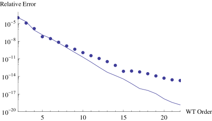
Figure 1: Behavior of the relative error achieved by the WT, versus the order $m$ [see Eq. (7)], when the Pearcey function is evaluated through the WT at the point $(x=7,y=\sqrt{2}(1+\mathrm{i}))$ (dots) and at the point $(x=-7,y=1)$ (solid curve).

Figure 1 shows the behavior of the relative error achieved by the WT, versus the order $m$ [see Eq. (7)], when the Pearcey function is evaluated through WT at the point $(x=7,y=\sqrt{2}(1+\mathrm{i}))$ (dots) and at the point $(x=-7,y=1)$ (solid curve). The first case corresponds to that presented by BH in their original paper,berryPRSA-91 while the second one has been treated by Paris and Kaminski.parisJCAM-06 The two cases differ by the number of saddles which contribute to the Pearcey integral, respectively one (complex) and three (reals). It is seen that in both cases the obtained accuracies are comparable to (and even better of) those obtained via the hyperasymptotics treatment. In particular, in the first case WT provides a relative error of the order of $10^{-15}$ for $m=20$, which is about 5 degree of magnitude better of that provided, on equal terms, by H.nota3 The ultimate relative error obtained via H (see Tab. 1 in Ref. berryPRSA-91, ) is of the order of $10^{-12}$, obtained with $m=25$, whereas WT provides, on equal terms, an error of $10^{-16}$ i.e., four degree of magnitude better. Moreover, in Ref. borghiOL-07, the same case was treated by using WT directly on the ascending power series of the Pearcey function, and it turned out that to achieve a relative error of $10^{-10}$ about 90 terms had to be considered in the partial sums sequence, whereas the same degree of accuracy is here reached with less than 10 terms. The example treated by Paris and Kaminski corresponds to the physical situation of a point located inside the cusp-shaped caustics, where the intensity distribution associated to the wavefield displays a typical fringe pattern, and WT produces results which are as accurate as those find in Ref. parisJCAM-06, (see Tab. 1 of that paper).

Before concluding the Letter, we want to give some warnings about possible limitations concerning the use of WT in asymptotics. We refer, in particular, to the fact that WT is not able, in the form given in Eq. (7), to resum nonalternating factorial divergent series, like the Euler series in Eq. (6) when $z$ is real and positive. nonalternating The above pathological situation occurs, for instance, when the Airy function Ai$(z)$ is required at the so-called Stokes lines, corresponding to complex value of $z$ such that $|\mathrm{arg}(z)|=2\pi/3$,berry234 where, on the contrary, the retrieving capabilities of H basically remain unchanged. We thus expect, in the general case, that the effectiveness of WT will depend on the position of the complex vector $\{x_{1},x_{2},...,x_{n-2}\}$ with respect to the Stokes lines and surfaces. wrightJPA-80 ; berry204 In this perspective, a deeper investigation about the retrieving capabilities of WT is required, but the preliminary results here presented seem to corroborate our initial feeling that Weniger transformation would be of great usefulness for the asymptotic treatment of several optical problems.

References

- (1) M. Born and E. Wolf, Principles of Optics, 7th ed. (Cambridge University Press, Cambridge, 1999).
- (2) G. Hardy, Divergent Series (American Mathematical Society, Chelsea Publishinh, Providence, RI, 1991).
- (3) “Divergent series are the invention of the devil, and it shameful to base on them any demonstration whatever” (Abel, 1828).
- (4) R. B. Dingle, Asymptotic Expansions: their Derivation and Interpretation (Academic Press, NY, 1973).
- (5) M. V. Berry and C. J. Howls, “Hyperasympotics,” Proc. R. Soc. Lond. A 430, 655-668 (1990).
- (6) M. V. Berry and C. Howls, “Hyperasymptotics for integrals with saddles,” Proc. R. Soc. Lond. A 434, 657-675 (1991).
- (7) G. Álvarez, C. J. Howls, and H. J. Silverstone “Dispersive hyperasymptotics and the anharmonic oscillator,” J. Phys. A: Math. Gen. 35, 4017 4042 (2002).
- (8) R. B. Paris and D. Kaminski, “Hyperasymptotic evaluation of the Pearcey integral via Hadamard expansions,” J. Comput. Appl. Math. 190, 437 452 (2006).
- (9) E. J. Weniger, “Nonlinear sequence transformations for the acceleration of convergence and the summation of divergent series,” Comput. Phys. Rep. 10, 189 (1989).
- (10) M. V. Berry and C. Upstill, “Catastrophe optics: morphologies of caustics and their diffraction patterns,” Prog. in Opt. XVIII, 257-346 (1980).
- (11) M. V. Berry, “Asymptotics, superasymptotics, hyperasymptotics,” in “Asymptotics beyond all orders”, H. Segur and S. Tanveer Eds. (Plenum, New York 1991), 1-14. (1992).
- (12) A. Erdélyi, Asymptotic Expansions (Dover, New York, 1956).
- (13) G. A. Baker, Jr. and P. R. Graves-Morris, Padé Approximants, 2nd Ed., (Cambridge University Press, Cambridge, 1996).
- (14) E. J. Weniger, “Mathematical properties of a new Levin-type sequence transformation introduced by Cìzek, Zamastil, and Skàla. I. Algebraic theory,” J. Math. Phys. 45, 1209 (2004).
- (15) E. J. Weniger, “Asymptotic Approximations to Truncation Errors of Series Representations for Special Functions,” arXiv:math/0511074v1 [math.CA]
- (16) R. Borghi, “Evaluation of diffraction catastrophes by using Weniger transformation,” Opt. Lett. 32, 226-228 (2007).
- (17) The formula we are referring is Eq. (42) of Ref. berryPRSA-91, , but the minus sign should be removed.
- (18) We are referring to Fig. 12 of Ref. berryPRSA-91, .
- (19) U. D. Jentschura, “Resummation of nonalternating divergent perturbative expansions,” Phys. Rev. D, 62, 076001 (2000).
- (20) F. J. Wright, “The Stokes set of the cusp diffraction catastrophe”, J. Phys. A 13, 2913-2928 (1980).
- (21) M. V. Berry and C. J. Howls, “Stokes surfaces of diffraction catastrophes of codimension three”, Nonlinearity 3, 281-291 (1990).