Quantum-statistical equation-of-state models: high-pressure Hugoniot shock adiabats

Abstract

We present a detailed comparison of two self-consistent equation-of-state models which differ from their electronic contribution: the atom in a spherical cell and the atom in a jellium of charges. It is shown that both models are well suited for the calculation of Hugoniot shock adiabats in the high pressure range (1 Mbar-10 Gbar), and that the atom-in-a-jellium model provides a better treatment of pressure ionization. Comparisons with experimental data are also presented. Shell effects on shock adiabats are reviewed in the light of these models. They lead to additional features not only in the variations of pressure versus density, but also in the variations of shock velocity versus particle velocity. Moreover, such effects are found to be responsible for enhancement of the electronic specific heat.

1 Introduction

The studies concerning matter under extreme conditions have broad applications to material science, inertial confinement fusion and astrophysics. About 98 % of the Universe is made of hot and ionized matter. The center of stars and white dwarfs have pressures exceeding thousands of Mbar and temperatures of tens of millions of K. In neutron stars pressures of millions of Mbar are believed to exist.

Nowadays, the shock-wave technique in laboratory laser experiments [1] enables one to reach maximum pressures that are as high as hundreds of megabars and even more for many materials [2]. Such pressures range to three orders of magnitude higher than the pressure in the Earth center and close to that in the center of the Sun.

Therefore, the need for suitable equation of state (EOS) of high-energy-density matter becomes crucial. The thermodynamics and the hydrodynamics of these systems can not be predicted without a knowledge of the EOS which describes how a material reacts to pressure. For instance, the theory of stellar evolution is affected by uncertainties in EOS (the internal structure and cooling time of the white dwarfs depend on the details of their EOS). More precisely, in astrophysical objects such as low-mass stars, brown dwarfs and giant planets, hydrogen and helium highly dominate, and their EOS, including non-ideality effects, can be accurately evaluated using “chemical” free-energy models (see for instance [3, 4, 5]). However, the EOS of carbon is also required for modeling inner envelopes of carbon-rich white dwarfs or outer accreted envelopes of neutron stars [6]. For general astrophysical applications of various types of stars, the EOS of oxygen is also required. In the center of the Sun, where matter density is about 157 g/cm³ and temperature 1.3 keV, although helium and hydrogen are the most abundant elements, the small quantity of iron has a strong impact on the calculation of the radiative opacity. Therefore, it is important to be able to determine the partial density of iron, which requires knowledge of its EOS.

In the present work, we consider strongly coupled (nonideal) plasmas, characterized by a high density and/or a low temperature. In such plasmas, ions are strongly correlated, electrons are partially degenerate, the De Broglie wavelength of the electron becomes of the same order of the interparticle distance, and the coupling parameter

$$\Gamma=\Big{(}\frac{4\pi}{3}\Big{)}^{1/3}\frac{Z^{*2}n_{i}^{1/3}}{k_{B}T},$$ (1)

ratio of Coulomb potential energy and thermal energy, is much larger than unity. The matter density $n_{i}$ represents the number of particles per volume unit, $Z^{*}$ the average ionization of the plasma, $k_{B}$ the Boltzmann constant and $T$ the temperature (throughout this paper, physical quantities are expressed in atomic units (a.u.)).

When a material is subjected to a strong shock wave, it becomes compressed, heated and ionized. As the strength of the shock is varied for a fixed initial state, the pressure-density final states of the material behind the shock belongs to a curve named shock adiabat or Hugoniot curve. The Hugoniot curve depends on the EOS of the matter, which, in principle, can be determined from theory. In practice, the barriers to ab initio calculations are formidable owing to the computational difficulty of solving the many-body problem. Consequently, it has proven necessary to introduce simplifying approximations into the governing equations. The price of simplification, however, is typically a loss of generality and the resulting theory is adequate only over a limited region of the phase diagram. The determination of the average electronic charge density relies usually on the Density Functional Theory. A well-known example is the Thomas-Fermi (TF) model of dense matter [7], which contains certain essential features in order to characterize the material properties over a limited range of conditions. At intermediate shock pressures, when the material becomes partially ionized, the EOS depends on the precise quantum-mechanical state of the matter, i.e. on the electronic shell structure [6, 8]. Therefore, there is a great interest in the physics of bound levels in high-energy-density plasmas [9] and quantum self-consistent-field (QSCF) models are replacing the TF approach. Such statistical models are well-suited for elements with a few occupied orbitals, i.e. with a “reasonable” number of electrons. Therefore, the theory presented in this paper is not applicable to hydrogen and helium, since their atomic number is too low. A lot of theoretical and computational efforts have been made in the United States and in Russia in the last twenty years concerning quantum effects on Hugoniot shock adiabats. It is important to review that huge amount of work, in the light of the most recent developments in the modeling of atomic structure. Indeed, QSCF calculations strongly depend on the modeling of the ions and on the treatment of free electrons. We present a QSCF-based EOS model, which will be named ESODE (Equation of State with Orbital Description of Electrons) in the following. The ionic contribution to the EOS is described by a perfect ideal gas, and the cold curve (T=0 K isotherm) has been obtained in most of the cases from Augmented Plane Wave (APW) calculations [10]. Exchange-correlation effects at finite temperature are taken into account. ESODE comes in two main versions for the thermal electronic contribution to the EOS: Average atom in a Spherical Cell (ASC) or Average atom in a Jellium of Charges (AJC). In both cases, bound electrons are treated quantum-mechanically. In the ASC model, all electrons are confined within a Wigner-Seitz sphere, and the continuity theorem of the wavefunctions at the boundary can be satisfied in different ways. In the AJC model, bound-electron wavefunctions can extend outside the sphere, where the plasma is represented by a uniform electronic density (jellium) neutralized by a continuous background of positive charges, representing ions. An interesting feature of AJC model is the possibility to use a quantum-mechanical description of free states (instead of a semi-classical one) together with a careful search for shape resonances. This seems to be necessary in order to ensure thermodynamic consistency, and a suitable description of polarization and density effects. The QSCF models (ASC and AJC) are described in section 2. Shock adiabats calculated from those models are presented, analyzed and compared to traditional TF model and to published experimental data in section 3. An interpretation of shell effect in terms of specific heat is discussed in section 3 as well. The dependence of shock velocity on particle velocity is analyzed in section 4.

2 The models

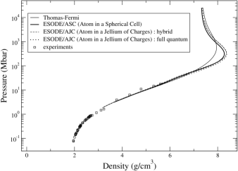
Figure 1: Hugoniot curves for Be. $\rho_{0}=$1.83 g/cm³. Experimental values are given by Refs. [32, 33, 34, 35, 36, 37].

2.1 First quantum statistical model: Atom in a Spherical Cell (ASC)

The task is to evaluate the contribution to the EOS coming from the excitations of the electrons due to temperature and compression. Atoms in a plasma can be idealized by an average atom confined in a Wigner-Seitz (WS) sphere, which radius $r_{ws}$ is related to matter density. Inside the sphere, the electron density has the following form [11]:

$$n(r) = \sum_{b}f_{l}(\epsilon_{b},\mu)\Big{|}\psi_{b}(\vec{r})\Big{|}^{2}$$ (2)

$$+\frac{\sqrt{2}(k_{B}T)^{3/2}}{\pi^{2}}[J_{1/2}\Big{(}-\bar{V}(r),\bar{\mu}-\bar{V}(r),\chi\Big{)}$$

$$+\chi J_{3/2}\Big{(}-\bar{V}(r),\bar{\mu}-\bar{V}(r),\chi\Big{)}],$$

where

$$f_{l}(x,y)=\frac{2(2l+1)}{1+\exp[(x-y)/k_{B}T]}$$ (3)

is the usual Fermi-Dirac population and

$$\tilde{J}_{n/2}(a,x,\sigma)=\int_{a}^{\infty}\frac{y^{n/2}(1+\sigma y/2)^{1/2}}{1+e^{y-x}}dy$$ (4)

is the modified Fermi function of order $n/2$. The first term in (2) corresponds to the contribution of bound electrons to the charge density, while the second term is the free-electron contribution, written in its semi-classical TF form. The energy $\epsilon_{b}$ and wavefunction $\psi_{b}$ of a bound orbital are calculated in the Pauli approximation [12], in which only first-order relativistic corrections to the Schrödinger equation

$$-\frac{1}{2}\Delta\psi_{b}+[V(r)+V_{mv}(r)+V_{D}(r)]\psi_{b}=\epsilon_{b}\psi_{b}$$ (5)

are retained. We introduce the notations $\chi=k_{B}T/E_{0}$, $E_{0}$ being the rest mass energy of the electron and $\bar{V}(r)=V(r)/(k_{B}T)$, where $V(r)$ is the self-consistent potential:

$$V(r)=-\frac{Z}{r}+\int_{0}^{r_{ws}}\frac{n(r^{\prime})}{|\vec{r}-\vec{r^{\prime}}|}d^{3}r^{\prime}+V_{xc}(r),$$ (6)

$V_{xc}$ being the exchange-correlation contribution, evaluated in the local density approximation [13]. V_mv is the mass-velocity correction

$$V_{mv}(r)=-\frac{[\epsilon_{b}-V(r)]^{2}}{2E_{0}}$$ (7)

and V_D the Darwin correction

$$V_{D}(r)=-\frac{1}{2}\frac{1}{2E_{0}+\epsilon_{b}-V(r)}\frac{dV}{dr}\Big{(}\frac{d}{dr}-\frac{1}{r}\Big{)}.$$ (8)

Omission of the spin-orbit term is a consequence of the spherical symmetry. Last, the chemical potential $\mu$ is obtained from the neutrality of the ion sphere:

$$\int_{0}^{r_{ws}}n(r)4\pi r^{2}dr=Z,$$ (9)

and $\bar{\mu}=\mu/(k_{B}T)$. Eqs. (2), (5), (6) and (9) must be solved self-consistently provided that, at each step of the iterative process towards convergence, bound orbitals are obtained from the Schrödinger equation. The electronic pressure $P_{e}$ [14, 15] consists of three contributions, $P_{e}=P_{b}+P_{f}+P_{xc}$, where the bound-electron pressure $P_{b}$ is evaluated using the stress-tensor formula

$$P_{b} = \sum_{b}\frac{f(\epsilon_{b},\mu)}{8\pi r_{ws}^{2}(1+\frac{\epsilon_{b}}{2E_{0}})}\Big{[}\Big{(}\frac{dy_{b}}{dr}\Big{|}_{r_{ws}}\Big{)}^{2}$$ (10)

$$+\Big{(}2\epsilon_{b}(1+\frac{\epsilon_{b}}{2E_{0}})-\frac{1+l+l^{2}}{r_{ws}^{2}}\Big{)}y_{b}^{2}(r_{ws})\Big{]},$$

$y_{b}$ representing the radial part of the wavefunction $\psi_{b}$ multiplied by $r$. The free-electron pressure $P_{f}$ reads

$$P_{f} = \frac{2\sqrt{2}}{3\pi^{2}}(k_{B}T)^{5/2}[\tilde{J}_{3/2}(-\bar{V}(r_{ws}),\bar{\mu}-\bar{V}(r_{ws}),\chi)$$ (11)

$$+\frac{\chi}{2}\tilde{J}_{5/2}(-\bar{V}(r_{ws}),\bar{\mu}-\bar{V}(r_{ws}),\chi)]$$

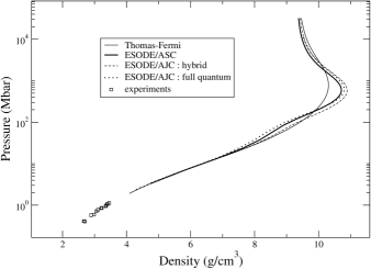
Figure 2: Hugoniot curves for B. $\rho_{0}=$2.34 g/cm³. Experimental values are given by Ref. [32, 35].

and $P_{xc}$ is the exchange-correlation pressure evaluated in the local density approximation [13]. The choice of the boundary conditions plays a major role in the expression of pressure. We chose a decreasing-exponential boundary condition, since it allows the matching of wavefunctions with Bessel functions outside the WS sphere [14], where the potential is zero. Moreover, such a condition is consistent with the fact that the bound-electron density vanishes at infinity. The internal energy in the ASC model is

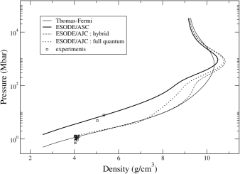
Figure 3: Hugoniot curves for C (graphite). $\rho_{0}=$2.28 g/cm³. Experimental values are given by Ref. [32, 35, 38, 39].

$$E_{e} = \sum_{j}n_{j}\epsilon_{j}-\frac{1}{2}\int_{0}^{r_{ws}}n(r)\int_{0}^{r_{ws}}\frac{n(r^{\prime})}{|\vec{r}-\vec{r^{\prime}}|}d^{3}rd^{3}r^{\prime}$$ (12)

$$+E_{xc}-\int_{0}^{r_{ws}}n(r)V_{xc}(n(r))d^{3}r,$$

where $E_{xc}$ is the exchange-correlation internal energy and $n_{j}$ the population of state $j$ (either bound or free). The first term in (12) can be expressed by

$$\sum_{j}n_{j}\epsilon_{k}=\sum_{b}f_{l}(\epsilon_{b},\mu)\epsilon_{b}+E_{f,k}+E_{f,p}.$$ (13)

$E_{f,p}$ is the potential energy

$$E_{f,p} = \frac{\sqrt{2}(k_{B}T)^{3/2}}{\pi^{2}}\int_{0}^{r_{ws}}[\tilde{J}_{1/2}(-\bar{V}(r),\bar{\mu}-\bar{V}(r),\chi)$$ (14)

$$+\chi\tilde{J}_{3/2}(-\bar{V}(r),\bar{\mu}-\bar{V}(r),\chi)]\bar{V}(r)d^{3}r$$

and $E_{f,k}$ the kinetic energy

$$E_{f,k} = \frac{\sqrt{2}(k_{B}T)^{5/2}}{\pi^{2}}\int_{0}^{r_{ws}}[\tilde{J}_{3/2}(-\bar{V}(r),\bar{\mu}-\bar{V}(r),\chi)$$ (15)

$$+\chi\tilde{J}_{5/2}(-\bar{V}(r),\bar{\mu}-\bar{V}(r),\chi)]d^{3}r.$$

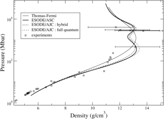
Figure 4: Hugoniot curves for Al. $\rho_{0}=$2.70 g/cm³. Experimental values are given by Ref. [32, 40, 41, 42, 43, 44, 45, 46, 47, 48].

In the present work, only non-relativistic calculations are carried out, which correspond to $E_{0}\rightarrow\infty$ in Eqs. (2), (10), (11), (14) and (15), in order to make comparisons with the model described below (in section 2.2), which is non-relativistic. Formulas (2) to (15) enable one to include relativistic effects without solving Dirac equation, in which the wavefunction consists of two components, making the choice of boundary conditions even more awkward.

2.2 Second quantum statistical model: Atom in a Jellium of Charges (AJC)

In order to go beyond the TF approximate treatment of continuum electron charge density, it is necessary to use a full quantum-mechanical description of the continuum states and to consider that both bound and free orbitals can extend outside the WS sphere. This leads us to define the environment outside and far from the central average ion. One way to address this is the jellium model (or electron gas model), i.e. a uniform electron density $-\bar{n}_{+}$ neutralized by a positive background $\bar{n}_{+}$ simulating the ionic charges. The model relies on a method proposed by J. Friedel [16, 17] in order to treat the electronic structure of an impurity, represented by a spherical potential of finite range, in an electron gas. It has been further developed by L. Dagens [18, 19] and F. Perrot [20, 21, 22]. In this framework, the electron density can be written:

$$n(r)=-\bar{n}_{+}+\Delta n_{a}+\Delta n_{ab}+\Delta n_{abc}+...,$$ (16)

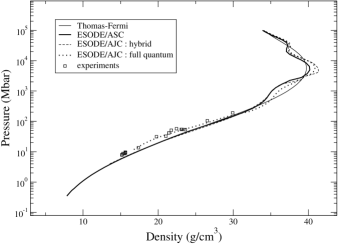
Figure 5: Hugoniot curves for Fe. $\rho_{0}=$7.85 g/cm³. Experimental values are given by Ref. [32, 40, 43, 49, 50, 51, 52, 53, 54, 55, 56, 57].

where $-\bar{n}_{+}$ is the density of the electron gas (jellium), $\Delta n_{a}$ the charge density displaced by the immersion of an atom “a” in the jellium, $\Delta n_{ab}$ the difference between the charge density of the $a-b$ molecule and the charge densities of free atoms $a$ and $b$, etc. The AJC approach retains only the first two terms. A nucleus of charge $Z$ is then introduced in a cavity in the positive background. The radius of the cavity represents the average atomic radius in the plasma. Therefore, the problem is reduced to the response of the electrons to the immersion of a positive charge $Z$. Ionic response is roughly simulated by the formation of a cavity. These considerations lead to the following form of the electron density:

$$n(r)=\sum_{b}f_{l}(\epsilon_{b},\mu)\Big{|}\psi_{b}(\vec{r})\Big{|}^{2}\\ +\sum_{l}\int_{0}^{\infty}f_{l}(\epsilon,\mu)\Big{|}\psi_{\epsilon,l}(\vec{r})\Big{|}^{2}d\epsilon,$$

where the eigenstates $(\psi_{b},\epsilon_{b})$ and the scattering states $(\psi_{\epsilon,l},\epsilon)$ are obtained solving Schrödinger equation with the potential

$$V(r)=-\frac{Z}{r}\int_{0}^{R_{\infty}}\frac{n(r^{\prime})}{|\vec{r}-\vec{r^{\prime}}|}d^{3}r^{\prime}+V_{xc}(r)-V_{xc}(-\bar{n}_{+}),$$ (17)

where $R_{\infty}>>r_{a}$, $r_{a}$ being the radius of the cavity. As in the ASC model, $V_{xc}$ is calculated from [13]. $V(r)$ is determined, as in the ASC model, in a self-consistent way. The ionic density is modeled by

$$n_{+}(r)=\left\{\begin{array}[]{ll}0&\mbox{for $r<r_{a}$}\\ \bar{n}_{+}&\mbox{for $r>r_{a}$.}\end{array}\right.$$ (18)

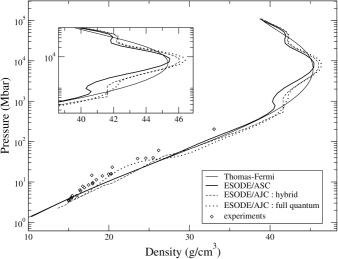
Figure 6: Hugoniot curves for Cu. $\rho_{0}=$8.84 g/cm³. Experimental values are given by Ref. [32, 34, 40, 43, 49, 56, 58, 59, 60, 61, 62, 63, 64, 65].

The expression of internal energy is [22]

$$E[n,n_{+}]=Z^{*}[e_{k}+e_{xc}](-\bar{n}_{+})+\Delta E[n,n_{+}]-\Lambda_{T}P_{1}v_{a},$$ (19)

with $v_{a}=4\pi r_{a}^{3}/3$, $\Lambda_{T}=(\partial\ln Z^{*}/\partial\ln T)|_{v_{a},T}$ and

$$P_{1}=\frac{\bar{n}_{+}}{v_{a}}\int_{r_{a}}^{R_{\infty}}4\pi r^{2}V(r)dr.$$ (20)

$e_{k}$ and $e_{xc}$ are the kinetic and exchange-correlation energies per free electron and $\Delta E[n,n_{+}]$ is the energy change resulting from the immersion of an ion in the jellium:

$$\Delta E[n,n_{+}] = \int_{0}^{R_{\infty}}(e_{k}[n(r)]-e_{k}[-\bar{n}_{+}])d^{3}r$$ (21)

$$-\int_{0}^{R_{\infty}}\frac{Z}{r}(n(r)+n_{+}(r))d^{3}r$$

$$+\frac{1}{2}\int_{0}^{R_{\infty}}\int_{0}^{R_{\infty}}\frac{n(r)+n_{+}(r)}{|\vec{r}-\vec{r^{\prime}}|}(n(r^{\prime})+n_{+}(r^{\prime}))d^{3}rd^{3}r^{\prime}$$

$$+\int_{0}^{R_{\infty}}(e_{xc}(n(r))-e_{xc}(-\bar{n}_{+}))d^{3}r.$$

The pressure is obtained by

$$P_{e}=[P_{k}+P_{xc}](-\bar{n}_{+})+\bar{n}_{+}U(r_{a})+(1-\Lambda_{v_{a},T})P_{1},$$ (22)

where $\Lambda_{v_{a}}=(\partial\ln Z^{*}/\partial\ln{v})|_{v_{a},T}$ and

$$U(r) = -\frac{Z}{r}+\frac{1}{r}\int_{0}^{r}4\pi r^{\prime 2}(n(r^{\prime})+n_{+}(r^{\prime}))dr^{\prime}$$ (23)

$$+\int_{r}^{R_{\infty}}4\pi r^{\prime}(n(r^{\prime})+n_{+}(r^{\prime}))dr^{\prime}.$$

The term $P_{k}$ corresponds to the pressure of a free-electron gas. The expression of pressure in (22) is rigorously the derivative of energy versus volume. This is the main difference with INFERNO model [23, 24]. The major difficulty of these models is that the average ionization is not well defined when the outer electrons are more or less delocalized. The only way to make the formalism variational is to specify the ionization in the AJC model. In other words, the question is how to define the residual electron density $(-\bar{n}_{+})$ far away from the point where the positive charge is introduced into the jellium. A convenient choice is $Z^{*}(v)=Z^{*}_{TF}(v)$ [22], $Z^{*}_{TF}$ being the TF ionization. In such a way derivatives of ionization with respect to volume and temperature can be obtained analytically, using the numerical fit proposed by R.M. More [25, 26].

ASC and AJC models are very different concerning the modeling of the environment of the atom, isolated and confined in the ASC model, and immersed in an infinite effective medium in the AJC model.

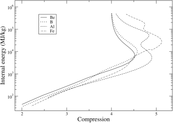
Figure 7: Internal energy versus compression along the Hugoniot curve for Be, B, Al and Fe in the ASC model.

2.3 Nuclear contribution and cold curve

The adiabatic approximation is used to separate the thermodynamic functions into electron and nuclear (ionic) components. The total pressure can be written:

$$P(\rho,T)=P_{c}(\rho)+P_{i}(\rho,T)+P_{t}(\rho,T),$$ (24)

where $P_{t}(\rho,T)=P_{e}(\rho,T)-P_{e}(\rho,0)$ is the thermal electronic contribution to the EOS, $P_{e}$ being electronic pressure. $P_{i}$ is the nuclear (ionic) pressure and $P_{c}$ the cold curve. The replacement of $P_{e}(\rho,0)$ by $P_{c}(\rho)$ is necessary since the results of the QSCF models are not valid for $T\rightarrow 0$. Following the same procedure, internal energy is divided into electronic, ionic and cold component. Expression (24) also holds for internal energy. The nuclear component is evaluated in the ideal-gas approximation.

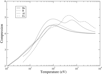
Figure 8: Compression versus temperature (thermodynamic path) along the Hugoniot curve for Be, B, Al and Fe in the ASC model.

$\bullet$ The cold curve must satisfy the condition that the quantity

$$\rho(\partial P/\partial\rho)$$ (25)

evaluated at normal density $\rho_{n}$ must be equal to the experimental bulk modulus $B_{0}$, which can be obtained from the sound velocity $c_{s}$ through $B_{0}=\rho c_{s}^{2}$. The cold curves are obtained either from APW [10] simulations, or using the Vinet [27] universal EOS. In the latter case, pressure can be evaluated analytically by

$$P_{c}=[3B_{0}(1-x)/x^{2}]\exp[\zeta(1-x)]$$ (26)

and the internal energy by

$$E_{c}=-\frac{9B_{0}}{\rho_{n}\zeta^{2}}[1-\exp[\zeta(1-x)][1-\zeta(1-x)]]$$ (27)

with $\zeta=3(B_{0}^{\prime}-1)/2$, $x=(\rho/\rho_{n})^{1/3}$ and $B_{0}^{\prime}=(\partial B_{0}/\partial P)|_{P=0,T}$. Values of such parameters obtained from experiments are available for several elements in the literature (see for instance [27, 28]). In many situations, Vinet EOS gives realistic results, and its accuracy is sufficient for most applications involving high pressures and temperatures.

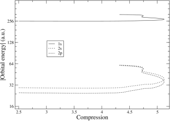
Figure 9: Absolute value of eigen-energy of orbitals 1s, 2s and 2p of Fe versus compression along the Hugoniot in the ASC model. For a given value of $\rho$, the corresponding value of $T$ can be found on Fig. 8.

3 Shock Hugoniots

3.1 Definitions

The initial state of the plasma is characterized by a density $\rho_{0}$, a temperature $T_{0}$, a pressure $P_{0}$, and an internal energy $E_{0}$. $D$ is the shock velocity, $u$ the matter velocity, $P$ and $E$ are respectively the pressure and internal energy behind the shock front. Since the mass preservation has to be satisfied, the density of the compressed gas $\rho$ satisfies the relation $\rho_{0}D=\rho(D-u)$. The resultant force acting on the compressed gas is equal to the difference of the pressure on the shock side and on the side of the undisturbed fluid, that is $P-P_{0}=\rho_{0}Du$. The increase in the sum of the internal and kinetic energies of the compressed gas is equal to the work done by the external force acting on the shock front, i.e. $\rho_{0}D(E-E_{0}+u^{2}/2)=Pu$. Rearranging these equations, one gets [29]:

$$\frac{1}{2}(P+P_{0})\Big{(}\frac{1}{\rho_{0}}-\frac{1}{\rho}\Big{)}=E-E_{0},$$ (28)

which is known as the Hugoniot relation. It is worth keeping in mind that the Hugoniot shock adiabat is not the collection of successive states of the matter during the propagation of the shock. The only relevant information is that the state of the matter “after the shock” belongs to the Hugoniot. Technically, the Hugoniot curve can be obtained by solving (28) at each temperature step, either calculating the EOS “in line” or by an interpolation in a table (pre-tabulated EOS). The two relations $P(\rho,T)$ and $E(\rho,T)$ constitute the EOS, which thermal part is calculated from the models described in sections 2.1 and 2.2.

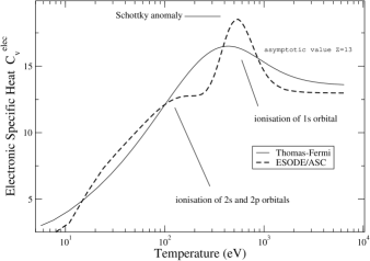
Figure 10: Electronic specific heat for Al.

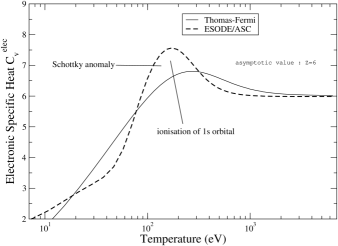
Figure 11: Electronic specific heat for C.

In this work, focus is put on the standard Hugoniot ($P_{0}$=0, $\rho_{0}$ equal to solid density and $T_{0}$=300 K). No distinction between $\rho_{0}$ and $\rho_{n}$ will be made in the following. As mentioned before, total energy is preserved during the shock, since an increase of internal energy is transformed into heat, which makes the temperature of the plasma increase. More exactly there is no heat exchange during the shock (which explains the name “shock adiabat”), but an increase of internal energy, distributed in internal degrees of freedom. One can wonder whether this conservation of energy is in contradiction with the fact that a physical system tends to minimize energy, as invoked in section 2. In classical mechanics, Noether’s theorem, which links symmetries and conservation laws, relates the invariance by translation in time to the conservation of total energy. Therefore, the idea that a physical system tends to minimize energy is often included in models where time is absent. This is also the case of the present study, since in QSCF models the wavefunctions are assumed to be time-independent. Therefore, only stationary solutions are considered here, and only systems in thermal equilibrium are supposed to exist. There is actually no contradiction: total energy is preserved during the shock, but the pressure calculated in the AJC_q model is thermodynamically consistent since it is calculated as a derivative of the energy (see (22) in section 2.2). Calculations have been performed for $T\leq$ 6.4 keV. Figures 1, 2, 3, 4, 5 and 6 represent Hugoniot curves for beryllium (Be, $Z$=4), boron (B, $Z$=5), carbon (C, $Z$=6), aluminum (Al, $Z$=13), iron (Fe, $Z$=26) and copper (Cu, $Z$=29) respectively, calculated from pure Thomas-Fermi EOS, ASC model, and AJC model with a full quantum treatment of electrons (namely AJC_q). The calculation within the jellium model with a hybrid description of electrons, i.e. where bound electrons are described in the framework of quantum mechanics and free electrons in the TF approximation, is also presented (AJC_h), since it is not equivalent to ASC model, even if it relies also on a hybrid description of electrons. The cold curve has been calculated using APW method for Be, C, Al, Fe and Cu. For Be, B, Al and Fe, Vinet universal EOS gives, for the Hugoniot curve, results which we find sufficiently accurate. For B, the Vinet parameters have been interpolated between Li ($Z$=3) and Be. All the QSCF models give very close results and differ from the TF approximation; it seems however that both hybrid models (atom in a spherical cell ASC or in a jellium of charges with quantum bound electrons and TF free electrons AJC_h) are very close to each other and differ from the full quantum atom-in-a-jellium-of-charges model AJC_q. For C, the Hugoniot curve obtained from ASC model is different from the ones obtained from other QSCF models, since the K shell is ionized for a lower density in the ASC approach, which induces a larger pressure. In the case of Al, the difference between the theories appears for $P\geq$ 3 Mbar and AJC_q gives higher pressures than the other models for 2$\leq\eta\leq$ 3.5, where $\eta=\rho/\rho_{0}$ is the compression rate. For $\eta\geq$ 3.5, all QSCF models give lower pressures than TF model.

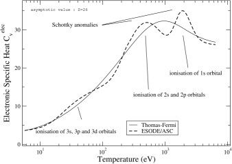
Figure 12: Electronic specific heat for Fe.

3.2 Quantum shell effects

Our models emphasize the thermodynamic domain where the Hugoniot curve strongly depends on the electronic structure, i.e. beyond four times solid density where the shoulders (double in the case of Al, Fig. 4) correspond to ionization of successive shells in the Average-Atom picture. The Hugoniot curve tends to the classical limit equal to four times the solid density at very high pressure, or typically $T>10$ keV. These shoulders are a consequence of the competition between the release of energy stocked as internal energy within the shells and the free-electron pressure. When ionization begins, the energy of the shock is used mainly to depopulate the relevant shells and the material is very compressive. However, the pressure of free electrons in increasing number dominates again and the material becomes more difficult to compress. Both models show compression maxima in the range $5\rho_{0}-6\rho_{0}$. In this region, the electrons from the ionic cores are being ionized and the shock density increases beyond the infinite pressure of $4\rho_{0}$. As ionization is completed, the plasma approaches an ideal gas of nuclei and electrons and the density approaches the fourfold density $4\rho_{0}$.

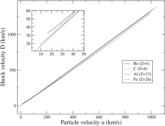
Figure 13: Shock velocity $D$ versus particle velocity $u$ for Be, C, Al and Fe.

The successive electron shells are accurately represented. For Be (Fig. 1), B (Fig. 2) and C (Fig. 3), all the models show a single density maximum, corresponding to the ionization of the K electron shell. For Al (Fig. 4), there are two density maxima corresponding to the K and L electron shells. For Fe (Fig. 5) and Cu (Fig. 6) there are density maxima or inflexions corresponding to the K, L and M electron shells. The L shell ionization feature gives the largest density increase. In the case of Cu (Fig. 6), the ASC and AJC_h models exhibit a kind of discontinuity around 40 g/cm³, due to pressure ionization of $2p$ orbital. Such a sharp increase of pressure does not exist in the AJC_q model, because of its thermodynamic consistency. This is due to the fact that it relies on a variational formulation: pressure is rigorously obtained as a derivative of the free energy, and shape resonances are carefully taken into account in the quantum treatment of free electrons. Such features lead to a continuous disappearing of a bound state into the continuum [30]. This is not the case of ASC and AJC_h models. In the framework of these two models, we tried to improve the dissolution of bound states into the continuum splitting them into bands and using a simple degeneracy reduction; this makes the discontinuity a little less sharp but does not solve the problem. Only a careful search of resonances would help, together with a variational calculation of pressure. Figure 7 illustrates the fact that internal energy also reflects the oscillations due to the shell structure, as well as the thermodynamic path $(T,\rho)$ (see the cases of Be, B, Al and Fe in Fig. 8). In fact, the non-monotonic character of thermodynamic variables stems from the eigen-energies of the orbitals themselves, which exhibit the oscillations as well (see Fig. 9). The first density for which a lower compression is obtained is named “turnaround” point.

Element	$a_{0}$ (km/s)	$a_{0}$ ([67])	$a_{1}$	$a_{1}$ ([67])	$a_{2}$ (s/km)
4Be	$9.137$	$/$	$1.147$	$/$	$5.70\;10^{-4}$
5B	$6.833$	$/$	$1.127$	$/$	$5.06\;10^{-3}$
6C	$10.437$	$/$	$0.940$	$/$	$5.06\;10^{-3}$
11Na	$9.718$	$/$	$1.063$	$/$	$9.58\;10^{-4}$
12Mg	$4.614$	$/$	$1.124$	$/$	$7.12\;10^{-4}$
13Al	$6.007$	$6.371$	$1.152$	$1.164$	$4.52\;10^{-4}$
26Fe	$6.675$	$6.982$	$1.144$	$1.190$	$8.42\;10^{-4}$
27Co	$5.348$	$/$	$1.150$	$/$	$7.96\;10^{-4}$
29Cu	$6.846$	$5.905$	$1.137$	$1.212$	$6.88\;10^{-4}$
40Zr	$6.926$	$/$	$1.125$	$/$	$3.28\;10^{-4}$
42Mo	$6.975$	$6.711$	$1.123$	$1.149$	$3.50\;10^{-4}$
48Cd	$3.676$	$4.251$	$1.180$	$1.182$	$9.07\;10^{-5}$

Table 1: Shock adiabat parameters of Be, B, C, Na, Mg, Al, Fe, Co, Cu, Zr, Mo and Cd. Coefficients $a_{0}$ and $a_{1}$ are compared with those published for metals in Ref. [67].

The pressure differences from the quantum mechanical theory along with the oscillatory feature at the turnaround density, can be explained by examining the heat capacity predicted by the TF and ASC theories along the Hugoniot path. At low temperature, the electronic heat capacity depends on the number of electrons that can be excited around the Fermi energy. The TF theory predicts a smooth increase since the density of states in this model is a monotonic function of energy. Therefore, the electronic specific heat

$$C_{v}^{elec}=\frac{1}{3k_{B}/2}\frac{\partial[E(\rho,T)-E_{i}(\rho,T)]}{\partial T}$$ (29)

is an interesting indicator of the ionization of successive shells and indirectly on the release of energy. Figure 10 represents $C_{v}^{elec}$ along the Hugoniot curve in the TF and in the ASC models for Al. Both theories show the effect of the coulomb attractive potential of the nucleus binding the electrons, represented by the peak around 300 eV for TF theory and 100 eV for ASC model. After the turnaround, there are 11 free electrons and 2 bound electrons remaining in the $1s$ orbital (K shell), which is far away from the energy zero (1.5 keV at T=100 eV). This phenomenon is a kind of Schottky anomaly [31]. As long as temperature is not sufficient to ionize those two electrons, the specific heat tends to an asymptote corresponding to an ideal gas of 11 independent particles. When both $1s$ electrons are ionized (after a “threshold” temperature), there is a sudden break in the specific heat, which tends to an ideal gas of 13 independent particles. It is not as important for the $2s$ and $2p$ bound states (L shell), since their energy levels are not as far from the continuum (a few tenth of eV). Figure 11 represents the electronic specific heat along the Hugoniot curve in the TF and in the ASC models for C. In that case, the only difference between both models is that there is a strong enhancement due to ionization of $1s$ orbital in the ASC approach, followed by the asymptotic limit of 6. The same phenomenon occurs with Fe (Fig. 12); in that case, after two Schottky anomalies, the electronic part of the specific heat tends to an ideal gas of 26 electrons.

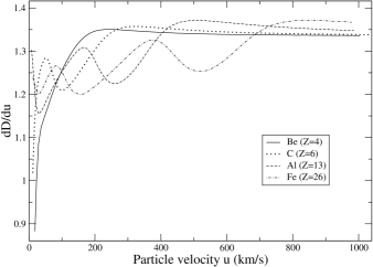
Figure 14: Derivative of shock velocity $dD/du$ versus particle velocity $u$ for Be, C, Al and Fe.

3.3 Comparisons with experimental data

Experimental data on Be [33, 34, 35, 36, 37], B [35], C [35, 38, 39], Al [40, 41, 42, 43, 44, 45, 46, 47, 48], Fe [40, 43, 49, 50, 51, 52, 53, 54, 55, 56, 57] and Cu [34, 40, 43, 49, 56, 58, 59, 60, 61, 62, 63, 64, 65] have been collected for comparison with the EOS models presented above. Several experimental methods have been used to generate well-defined shock states: gas guns for pressures up to 5 Mbar, explosive-driven spherical implosions and laser-driven plane waves for generating shocks up to 10 Mbar. High-power lasers are capable of driving multimegabar shocks in small samples either by direct irradiation or indirectly. In the latter case, the target is mounted on a hohlraum into which the lasers are focused. Pressures up to a few Gbar have been reached through underground nuclear explosions. If the shocks have been measured accurately, superimposing all of these data should yield a single smooth shock Hugoniot curve. The maximum pressures reached in the experiments are: 18 Mbar for Be, 4000 Mbar for Al, 191 Mbar for Fe and 204 Mbar for Cu. It appears difficult to decide which model gives the best agreement with experiments, since there are obviously very few available data for the region of interest (typically above 100 Mbar). The error bars associated to the ultrahigh-pressure experimental values for Al are too large to conclude concerning the existence of shell effects. For Fe and Cu, results from AJC_q model seem to agree better with the first interpretable experimental points than the hybrid models (ASC or AJC_h). The large errors in the measurements make the experimental results useless for refining the theoretical data. Therefore, it is not really legitimate to attempt to relate gas-dynamics measurements with a discussion of shell effects. Anyway, analysis of the computational results shows that the deviation from the experimental points of Al can not be explained only by shell effects. In the region where most of the experimental points are available, the role of the cold component is important, while shell effects begin to play a significant role after the matter is already compressed (around the asymptotic compression $\eta\approx 4$) and begins to heat up. In order to discriminate models from eachother, the uncertainty on velocities should be very small (typically $\leq$ 1%), which is not possible. However, if the temperature beyond the shock could be measured with an incertainty of about 20 %, it should be possible to decide which model gives the best agreement with experimental data in the $(T,P)$ plane.

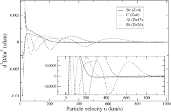
Figure 15: Second derivative of shock velocity $d^{2}D/du^{2}$ versus particle velocity $u$ for Be, C, Al and Fe.

4 Shock and particle velocities

The particle and shock velocities read (see section 3.1):

$$u=\sqrt{\frac{(\rho-\rho_{0})(P-P_{0})}{\rho_{0}\rho}}\;\;\mbox{and}\;\;D=\sqrt{\frac{\rho(P-P_{0})}{\rho_{0}(\rho-\rho_{0})}}.$$ (30)

Expressions in (30) are generic; they do not involve, a priori, any explicit relation $D(u)$. However, one has [66]:

$$D=c_{s}+\frac{\Lambda_{0}}{2}u+\frac{\Lambda_{0}}{6c_{0}}\Big{[}\frac{G_{0}}{2}-\frac{1}{\rho_{0}}\frac{P_{0}^{(3)}}{P_{0}^{(2)}}-\frac{9}{4}\Lambda_{0}\Big{]}u^{2}+O(u^{3}),$$ (31)

where $G_{0}$ is the Grüneisen coefficient at $\rho=\rho_{0}$,

$$\Lambda_{0}=-P_{0}^{(2)}/(2\rho_{0}P_{0}^{(1)})$$ (32)

and

$$P^{(n)}=(\partial^{(n)}P/\partial(1/\rho)^{(n)})|_{S}.$$ (33)

For a perfect ideal gas, the Grüneisen parameter $(\partial P/\partial E)|_{\rho}/\rho$ tends to $2/3$. Expression (31) is suitable for densities close to the pole $(\rho_{0},T_{0},P_{0},E_{0})$, since it comes from a Taylor development of $D$ and $u$ around that specific initial point. For metals, it is often invoked that the relation is quasi-linear. Figure 13 illustrates the fact that the $(u,D)$ relationship is almost linear over a wide range of densities, except close to the origin, where we could not perform the calculation. It is interesting to try to fit the $(u,D)$ relation with a quadratic expression [67] $D=a_{2}u^{2}+a_{1}u+a_{0}$. The parameters are presented in table 1 for Be, B, C, Na, Mg, Al, Fe, Co, Cu, Zr, Mo and Cd, and compared to the values published by Al’tshuler et al [67]. The slope is different from $4/3$, corresponding to the perfect ideal gas, as can be checked from (30). However, if one looks more carefully at the first and second derivatives (Figs. 14 and 15) of shock velocity versus particle velocity, one finds that the behaviour of shock velocity is more complicated, and that there are some oscillations, reflecting the shell structure as well, and even inflexion points (see Fig. 15). The amplitude of oscillations in the $(u,D)$ relationship is very small, which is not the case of $(\rho,P)$ relationship. This is even more sensitive at the turnaround of the shock adiabat. Indeed, in that case, $(\partial P/\partial\rho)|_{S}$ has strong variations, which implies, according to the relation

$$\rho^{2}\frac{\partial P}{\partial\rho}\Big{|}_{S}+P\frac{\partial P}{\partial E}\Big{|}_{\rho}=\rho^{2}\frac{\partial P}{\partial\rho}\Big{|}_{E},$$ (34)

that $P$ has strong variations as well, since $(\partial P/\partial E)|_{\rho}$ and $(\partial P/\partial\rho)|_{E}$ have smooth variations. A survey of Figs. 13, 14 and 15 shows download curvature, upward curvature and more complicated deviations from non-linear behaviour. G.I. Kerley [68] suggests that it is more convenient to plot $(D-u)$ versus $u$ instead of $D$ versus $u$. His analysis concerns mostly low velocities, typically below 10 km/s, but Fig. 16 shows that it remains relevant for high velocities in the region affected by shell effects and confirms our results.

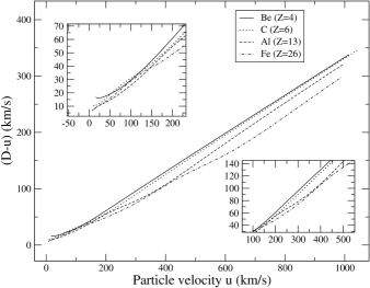
Figure 16: $(D-u)$ versus $u$ for Be, C, Al and Fe.

5 Conclusion

The application of shock waves to plasma physics makes possible the generation under laboratory conditions of extremely high energy densities typical of astrophysical objects such as stars and giant planets. The physical information obtained this way extends our basic knowledge on physical properties of plasma to a broad area of the phase diagram up to pressures nine orders of magnitude higher than the atmospheric one.

We presented and compared two equation-of-state models in which the thermal electronic contribution is evaluated using two different quantum self-consistent-field models: the atom in a spherical cell (ASC) and the atom in a jellium of charges (AJC). It was shown that both models are very well suited for the calculation of high-pressure Hugoniot shock adiabats and that the AJC model, relying on a full quantum treatment of the electrons, provides a better treatment of pressure ionization.

We proposed a qualitative and quantitative study of quantum orbital effects on the principal shock adiabat for different elements, In the $(\rho,P)$, $(\rho,E)$ and $(T,\rho)$ representations, such effects lead to oscillations corresponding to the ionization of successive orbitals. We found that such oscillations are also visible in the electronic specific heat, through Schottky anomalies, and in the energies of the orbitals themselves. They are responsible for deviations from linear behaviour in the relationship between shock velocity and particle velocity.

The next step will be to check whether the oscillations still exist “beyond” the Average Atom model, i.e. if real electronic configurations are taken into account [14, 15]. The remaining difficulty of our models comes from the impossibility to represent in a simple and suitable way the influence of the plasma environment on a specific ion. Indeed, such an environment fluctuates; the number, the localization in space and the structure of neighbouring ions may change drastically. In principle, it should be necessary to calculate a large number of geometric configurations of the system (positions of ions in space), and then their thermodynamic average. Such an approach is untractable ab initio, except for very low-$Z$ atoms in a restricted range of temperature and density, using molecular-dynamics simulations [69].

References

- [1] B.A. Remington, D. Arnett, R.P. Drake and H. Takabe (1999) Science 284, 1488 (1999).
- [2] W.J. Nellis, Contrib. Plasma Phys. 45(3-4), 243 (2005).
- [3] C. Winisdoerffer and G. Chabrier, Phys. Rev. E 71, 026402 (2005).
- [4] H. Juranek, V. Schwarz and R. Redmer, J. Phys. A: Math. Gen. 36, 6181 (2003).
- [5] H. Juranek, R. Redmer and W. Stolzmann, Contrib. Plasma Phys. 41, 131 (2001).
- [6] A.Y. Potekhin, G. Massacrier and G. Chabrier, Phys. Rev. E 72, 046402 (2005).
- [7] R.P. Feynman, N. Metropolis and E. Teller, Phys. Rev. 75, 1561 (1949).
- [8] M.P. Desjarlais, Contrib. Plasma Phys. 45(3-4), 300 (2005).
- [9] W. Ebeling, W. Kraeft and D. Kremp Theory of Bound States and Ionization Equilibrium in Plasmas and Solids, Ackademie-Verlag, Berlin (1976).
- [10] T.L. Loucks Augmented Plane Wave Method: A Guide to Performing Electronic Structure Calculations, W.A. Benjamin, Inc., New York (1972).
- [11] B.F. Rozsnyai, Phys. Rev. A 5, 231 (1972).
- [12] H.A. Bethe and E.E. Salpeter Quantum Mechanics of One- and Two-electron Atoms, Springer Verlag, Berlin (1957).
- [13] H. Iyetomi and S. Ichimaru, Phys. Rev. A 34, 433 (1986).
- [14] J.C. Pain, G. Dejonghe and T. Blenski, J. Quant. Spectrosc. Radiat. Transfer 99, 451 (2006).
- [15] J.C. Pain, G. Dejonghe and T. Blenski, J. Phys. A: Math. Gen. 39, 4659 (2006).
- [16] J. Friedel, Philos. Mag. 43, 153 (1952).
- [17] J Friedel, Adv. Phys. 3, 446 (1954).
- [18] L. Dagens, J. Phys. C 5, 2333 (1972).
- [19] L. Dagens, J. Phys. (Paris) 34, 879 (1973).
- [20] F. Perrot, Phys. Rev. A 42, 4871 (1990).
- [21] F. Perrot, Phys. Rev. E 47, 570 (1993).
- [22] F. Perrot, Recherche d’un modèle de structure électronique des plasmas applicable aux calculs d’opacité et d’équation d’état (1998), unpublished.
- [23] D.A. Liberman, Phys. Rev. B 20, 4981 (1979).
- [24] B.F. Rozsnyai, J.R. Albritton, D.A. Young, V.N. Sonnad and D.A. Liberman, Phys. Lett. A 291, 226 (2001).
- [25] R.M. More Atomic Physics in Inertial Confinement Fusion, UCRL Report 84991 (1981).
- [26] Salzmann D Atomic Physics in Hot Plasmas, International series of monographs on physics, New York, Oxford University Press, p 28 (1998).
- [27] P. Vinet, J.H. Rose, J. Ferrante and J.R. Smith, J.Phys.: Condens. Matter 1, 1941 (1989).
- [28] A. Dewaele, P. Loubeyre and M. Mezouar, Phys. Rev. B 70, 094112 (2004).
- [29] Ya.B. Zel’dovich and Yu.P. Raizer, Physics of Shock Waves and High-Temperature Hydrodynamic Phenomena, Academic Press, New York, Vol 1, Ch 3 (1966).
- [30] W. Kohn and C. Majundar, Phys. Rev. 140, A1133 (1965).
- [31] W. Schottky, Physik. Z. 23, 448 (1922).
- [32] A.V. Bushman, I.V. Lomonosov, K.V. Khishchenko, Shock Wave Database and references therein (http://teos.ficp.ac.ru/rusbank/).
- [33] J.M. Walsh, M.H. Rice, R.G. McQueen, F.L. Yarger, Phys. Rev. 108, 196 (1957).
- [34] W.H. Isbell, F.H. Shipman, A.H. Jones, Hugoniot equation of state measurements for eleven materials to five megabars, General Motors Corp. Materials Science Laboratory Report MSL-68-13 (1968).
- [35] S.P. March, LASL Hugoniot Data, University of California Press, Berkeley, 1980.
- [36] C.E. Ragan, Phys. Rev. Ser. A 25, 3360 (1982).
- [37] W.J. Nellis, J.A. Moriarty, A.C. Mitchell, N.C. Holmes, J. Appl. Phys. 82, 2225 (1997).
- [38] W.H. Gust, Phys. Rev. B 22, 4744 (1980).
- [39] W.J. Nellis, A.C. Mitchell, A.K. McMahan, J. Appl. Phys. 90, 696 (2001).
- [40] L.V. Al’tshuler, N.N. Kalitkin, L.V. Kuz’mina, B.S. Chekin, Zh. Eksp. Teor. Fiz. 72, 317 (1977), Sov. Phys. JETP 45, 167 (1977).
- [41] L.P. Volkov, N.P. Voloshin, A.S. Vladimirov, V.N. Nogin, V.A. Simonenko, Pis’ma Zh. Eksp. Teor. Fiz. 31, 623 (1980), JETP Lett. 31, 588 (1980).
- [42] A.S. Vladimirov, N.P. Voloshin, V.N. Nogin, A.V. Petrovtsev, V.A. Simonenko, Pis’ma Zh. Eksp. Teor. Fiz. 39, 69 (1984), JETP Lett. 39, 85 (1984).
- [43] C.E. Ragan, Phys. Rev. Ser. A 29, 1391 (1984).
- [44] V.A. Simonenko, N.P. Voloshin, A.S. Vladimirov, A.P. Nagibin, V.N. Nogin, V.A. Popov, V.A. Vasilenko, Yu.A. Shoidin, Zh. Eksp. Teor. Fiz. 88, 1452 (1985), Sov. Phys. JETP 61, 869 (1985).
- [45] E.N. Avrorin, B.K. Vodolaga, N.P. Voloshin, V.F. Kuropatenko, G.V. Kovalenko, V.A. Simonenko, B.T. Chernodolyuk, Pis’ma Zh. Eksp. Teor. Fiz. 43, 241 (1986), JETP Lett. 43, 309 (1986).
- [46] M.A. Podurets, V.M. Ktitorov, R.F. Trunin, L.V. Popov, A.Ya. Matveev, B.V. Pechenkin, A.G. Sevast’yanov, Teplofiz. Vys. Temp. 32, 952 (1994).
- [47] R.F. Trunin, N.V. Panov, A.B. Medvedev, Pis’ma Zh. Eksp. Teor. Fiz. 62, 572 (1995).
- [48] M.D. Knudson, R.W. Lemke, D.B. Hayes, C.A. Hall, C. Deeney, J.R. Asay, J. Appl. Phys. 94, 4420 (2003).
- [49] L.V. Al’tshuler, A.A. Bakanova, R.F. Trunin, Zh. Eksp. Teor. Fiz. 42, 91 (1962), Sov. Phys. JETP 15, 65 (1962).
- [50] K.K. Krupnikov, A.A. Bakanova, M.I. Brazhnik, R.F. Trunin, Dokl. Akad. Nauk SSSR 148, 1302 (1963), Sov. Phys. Dokl. 8, 205 (1963).
- [51] L.V. Al’tshuler, B.N. Moiseev, L.V. Popov, G.V. Simakov, R.F. Trunin, Zh. Eksp. Teor. Fiz. 54, 785 (1968), Sov. Phys. JETP 27, 420 (1968).
- [52] R.F. Trunin, M.A. Podurets, G.V. Simakov, L.V. Popov, B.N. Moiseev, Zh. Eksp. Teor. Fiz. 62, 1043 (1972), Sov. Phys. JETP 35, 550 (1972).
- [53] L.V. Al’tshuler, A.A. Bakanova, I.P. Dudoladov, E.A. Dynin, R.F. Trunin, B.S. Chekin, Zh. Prikl. Mekh. Tekhn. Fiz. 2, 3 (1981), J. Appl. Mech. Techn. Phys. 22, 145 (1981).
- [54] R.F. Trunin, M.A. Podurets, L.V. Popov, V.N. Zubarev, A.A. Bakanova, V.M. Ktitorov, A.G. Sevast’yanov, G.V. Simakov, I.P. Dudoladov, Zh. Eksp. Teor. Fiz. 102, 1433 (1992), Sov. Phys. JETP 75, 777 (1992).
- [55] R.F. Trunin, M.A. Podurets, L.V. Popov, B.N. Moiseev, G.V. Simakov, A.G. Sevast’yanov, Zh. Eksp. Teor. Fiz. 103, 2189 (1993), JETP 76, 1095 (1993).
- [56] R.F. Trunin, Usp. Fiz. Nauk 164, 1215 (1994).
- [57] L.V. Al’tshuler, R.F. Trunin, K.K. Krupnikov, N.V. Panov, Usp. Fiz. Nauk 164, 575 (1996), Sov. Phys. Usp. 39, 539 (1996).
- [58] L.V. Al’tshuler, S.B. Kormer, A.A. Bakanova, R.F. Trunin, Zh. Eksp. Teor. Fiz. 38, 790 (1960), Sov. Phys. JETP 11, 573 (1960).
- [59] S.B. Kormer, A.I. Funtikov, V.D. Urlin, A.N. Kolesnikova, Zh. Eksp. Teor. Fiz. 42, 686 (1962), Sov. Phys. JETP 15, 477 (1962).
- [60] R.F. Trunin, M.A. Podurets, B.N. Moiseev, G.V. Simakov, L.V. Popov, Zh. Eksp. Teor. Fiz. 56, 1172 (1969), Sov. Phys. JETP 29, 630 (1969).
- [61] R.F. Trunin, M.A. Podurets, G.V. Simakov, L.V. Popov, B.N. Moiseev, Zh. Eksp. Teor. Fiz. 62, 1043 (1972), Sov. Phys. JETP 35, 550 (1972).
- [62] L.V. Al’tshuler, B.S. Chekin, Metrology of high pulsed pressures, in: Proceed. of 1st All-Union Pulsed Pressures Simposium (VNIIFTRI, Moscow, 1974) 1, 5.
- [63] B.L. Glushak, A.P. Zharkov, M.V. Zhernokletov, V.Ya. Ternovoi, A.S. Filimonov, V.E. Fortov, Zh. Eksp. Teor. Fiz. 96, 1301 (1989), Sov. Phys. JETP 69, 739 (1989).
- [64] A.C. Mitchell, W.J. Nellis, J.A. Moriarty, R.A. Heinle, N.C. Holmes, R.E. Tipton, G.W. Repp, J. Appl. Phys. 69, 2981 (1991).
- [65] R.F. Trunin, L.A. Il’kaeva, M.A. Podurets, L.V. Popov, B.V. Pechenkin, L.V. Prokhorov, A.G. Sevast’yanov, V.V. Khrustalev, Teplofiz. Vys. Temp. 32, 692 (1994).
- [66] F. Chaissé Propriétés structurales de la courbe d’Hugoniot, CEA Report R-6013 (2002).
- [67] L.V. Al’tshuler, R.F. Trunin, V.D. Urlin, V.E. Fortov and V.E. Funtikov, Sov. Phys. Usp. 42, 261 (1999).
- [68] G.I. Kerley, The linear Relation in Shock-Wave Physics, Research Report KTS06-1, Kerley Technical Services, P.O. Box 709, Appomattox, VA 24522-0709) (2006).
- [69] R. Car and M. Parrinello, Phys. Rev. Lett., 55, 2471 (1985).