Mesoscopic fluctuations of spin currents

Abstract

Spin currents may be generated by applying bias voltages $V$ to the nanostructures even in the absence of spin-active ferromagnetic interfaces. Most theoretical proposals concentrate on a concrete spin-orbit interaction and on the disorder-averaged effect. It remains underappreciated that any spin-orbit interaction produces random spin currents with a typical amplitude $\simeq e^{2}V/\hbar$ not affected by disorder. This work addresses such mesoscopic fluctuations of spin currents for generic model of a nanostructure where several quantum connectors meet in a single node. The analysis is performed in the framework of recently developed quantum circuit theory of $G_{Q}$ corrections and reveals four distinct mechanisms of spin current fluctuations. The results are elaborated for simple models of tunnel and ballistic connectors.

1 Introduction

In recent years considerable theoretical and experimental work is aimed at the controlled manipulation of electron spin in (nanoscale) solid state systems, a field commonly referred to as spintronics [1]. Spin current defined as a flow of electron spin is one of the central and most useful concepts of this field.[2] Much confusion can be easily brought by irresponsible and/or uncareful use of this concept. This confusion is related to two facts. Firstly, spin currents, unlike electric or particle currents, are not usually conserved under interesting circumstances. Secondly, it is frequently not evident that the spin currents due to electrons near Fermi surface really present a dominant contribution in spin balance: This is certainly not true for equilibrium and/or electrically isolated systems.

Therefore, it seems prudent to start the article with a short description of the measurement that can directly access such spin current [3] and/or its temporal fluctuations[4] Let us consider a current injector of the resistance $R$ that pushes spin-polarized electrons into a metallic lead. In principle, this polarization disappears far in the lead. However, spin relaxation is usually a slow process so the spin current is preserved at significant distance $L_{sf}$ from the injector. Let us set up a spin-active interface within this distance from the injector. A spin-active interface provides different resistance for electrons of two different spin projection on the polarization axis of the interface. Most common example is the interface between a ferromagnetic and non-ferromagnetic metal. In this case, the polarization axis coincides with the direction of magnetization of the ferromagnet.

The voltage drop over the interface is thereby sensitive to spin of the electrons that traverse it. We would like the difference of the voltage drops at opposite directions of the polarization axis is directly proportional to the projection of the spin current on the polarization axis. This enables the measurement of spin current as a voltage measurement. To achieve this, one has to choose the interface resistance $R_{in}$ such that $R_{in}\ll R$ but still by far exceeds the resistance of the metal piece between the injector and the interface. We shall stress the useful analogy between spin current and spin accumulation, on one side, and electric current and voltage on another side. The above condition on $R_{in}$ is precisely the same as the condition for the measuring the electric current from the injector through the voltage drop over the interface.

The disadvantage of this measurement scheme is that at a given polarization of the interface only a single projection of the spin current can be measured. The point is that the spin current with the projection perpendicular to the polarization axis is usually immediately adsorbed at the interface.[2] An alternative scheme [5] where all three components of the spin current can be measured in the least obtrusive way is still difficult to realize for solid-state devices.

Spin currents in the systems where spin-active interfaces dominate the resistance, are well-studied. [2] Usually, a simple circuit-theory approach based on the balance of spin and charge currents [6] suffices to describe everything. Here, we consider the situation where there are no spin-active interfaces in the nanostructure used as an injector of the spin current. Still there is spin-orbit interaction.

It was noticed quite long ago [7] that in bulk homogeneous materials without inversion center electric currents produce spin currents. However, in bulk materials this effect is usually negligible in comparison with other agents of spin orientation, for instance, with the effect of magnetic field produced by the currents.[8] In ballistic nanostructures, the spin-orbit interaction in combination with geometric effects may lead to spin currents. Consider, for instance, a single isotropic scattering center subject to electron flow in $z$ direction. Intensity of electron scattering to $+x$ and $-x$ directions will depend on the spin projection on $y$ axis. If we direct the scattered electrons to different terminals, we get spin currents in the terminals. Such device proposal has been actually elaborated.[9] At more abstract microscopic level, spin-orbit interaction always results in a spin-dependent scattering matrix (see, for instance, [10]). However, since the effect relies on geometry, it is drastically decreased by any scattering in the nanostructure. Indeed, the scattering makes electron distribution function isotropic so that they forget the geometry. In scattering matrix language, the spin currents are determined by random phase shifts of the scattering amplitudes. After averaging over random phase shifts, the average spin current is supposed to average out if the scattering is sufficiently chaotic. This has been confirmed by extensive numerical experiments.[11]

It remains underappreciated that even for completely chaotic scattering there must be significant mesoscopic fluctuations of spin currents. They are governed by the same quantum interference mechanism as the celebrated Universal Conductance Fluctuations [12] and must be of the same scale. Such fluctuations are clearly seen in numerical simulations at quantum level [13]. Recent numerical work [14] provides a detailed study of these fluctuations for a concrete device.

In this work, we theoretically investigate the mesoscopic fluctuations of spin currents for multi-terminal nanostructures assuming sufficient isotropization of electron distribution function that allows to disregard all geometric effects. This means that after averaging over random phase shifts/impurity positions there is no net spin effect and the system is $SU(2)$ invariant with respect to rotations in spin space. Under these conditions, spin-orbit interaction only manifest itself in spin relaxation and completely characterized by the rate of such relaxation. We denote the full spin current with spin index $\alpha=1,2,3$ coming to the terminal $i$ as $I^{\alpha}_{i}$. We study the correlators of the two,

$$\langle\!\langle I^{\alpha}_{i}I^{\beta}_{j}\rangle\!\rangle=\delta_{\alpha\beta}I_{ij}$$

that are $SU(2)$ invariant.

We stress that we study spin current fluctuations that persist at least at the scale of the contact size. This is very different from mesoscopic fluctuations of spin accumulation. Such fluctuations are known to form a random pattern correlated at the scale of mean free path [15, 16] and are disregarded here.

2 Model, parameters, expectations

We model a nanostructure along the lines of quantum circuit theory [17, 18] representing a complicated setup in terms of three kinds of the elements: terminals, nodes, and connectors. An arbitrary nanostructure with sufficiently chaotic scattering inside can be presented in this way with using sufficiently many nodes and connectors.

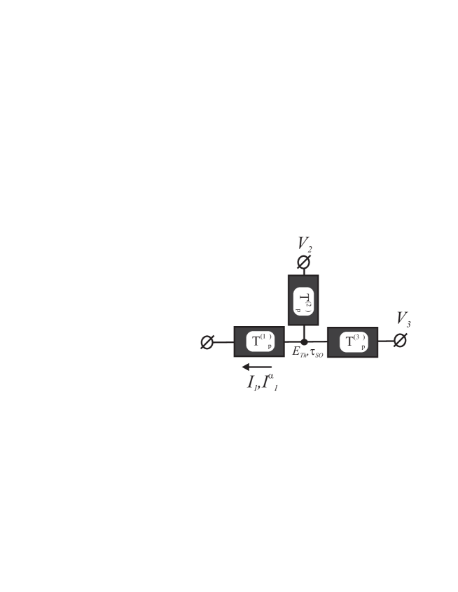
Figure 1: Generic model of nanostructure. We consider a multi-terminal setup (three terminals shown in the Figure). The connectors are characterized by the sets of transmission eigenvalues ($T^{(i)}_{p}$). The node is characterized by Thouless energy related to the electron dwell time in the node. The spin-orbit interaction is represented by $\tau_{SO}$, spin relaxation time in the node.

The specific model under consideration consists of a single node attached to many reservoirs by arbitrary connectors (Fig. 1). The node in circuit theory is very close to ”chaotic cavity” used in Random Matrix Theory (RMT) of quantum transport. [19]

The connector $i$ is characterized by a set of transmission eigenvalues $T^{(i)}_{p}$, $p$ labelling quantum channels in the connector. Conductance of the connector reads $G^{(i)}=G_{Q}\sum_{p}T^{(i)}_{p}$. In the limits of applicability of the circuit theory, $G^{(i)}_{T}\gg G_{Q}$. There is a single terminal per connector most generally characterized by an energy-dependent electron filling factor $f_{i}(E)$. The mesoscopic fluctuations of two-terminal conductance in this model have been considered in [20] by RMT methods.

Spin current fluctuations can not be accessed by RMT since, as we will see, they disappear in the limit of pure ensembles. We need more parameters that are absent in RMT but present in more detailed and microscopic theories [12] that describe transitions between the ensembles. The size of the node is characterized by the mean level spacing $\delta_{S}$, or, more adequately, by the Thouless energy $E_{th}\equiv G_{\Sigma}\delta_{S}/G_{Q}$, $G_{\Sigma}\equiv=\sum_{i}G^{(i)}_{T}$. Mesoscopic fluctuations are supposed to correlate at energies $\simeq E_{th}$. For the present purposes, the most important parameter is the spin-orbit time $\tau_{SO}$ that determines spin relaxation in the node. We assume no spin-orbit effects in the connectors. Therefore, $\tau_{SO}$ contains all information concerning the spin-orbit interaction and its strength is given by a dimensionless $\eta_{SO}\equiv\hbar/\tau_{SO}E_{th}$.

At moderate values of this parameter, $\eta_{SO}\simeq 1$, we expect the mesoscopic fluctuations of spin current to be very similar to the mesoscopic fluctuations of the charge current. Those are known to be universal corresponding to the fluctuating conductance of the order of $G_{Q}$. At low voltages $eV\ll E_{th}$ this gives $\langle\!\langle I^{2}\rangle\!\rangle\simeq G^{2}_{Q}V^{2}$ while at large voltages $eV\gg E_{th}$ $\langle\!\langle I^{2}\rangle\!\rangle\simeq G^{2}_{Q}VE_{th}/e$ [21]. The distinction is that the spin current is not conserved. Therefore, we expect non-zero fluctuations of the total spin current $I_{\alpha}=\sum_{i}I^{(i)}_{\alpha}$ to/from the nanostructure. Those must be of similar magnitude as the fluctuations of the current to/from a reservoir.

Naturally, we expect the spin current fluctuations to vanish in the limit $\eta_{SO}\ll 1$ of weak spin-orbit interaction. The opposite limit is less obvious: One might think that strong spin-orbit interaction leads to fast spin relaxation in the node, the latter obviously suppresses any spin effects.

The results derived and discussed in the article conform to these general expectations and give details of spin current fluctuations and their correlations for connectors of low and high transmission.

3 Circuit-theory action

Qualitatively, the model is most conveniently described by the action ${\cal S}$ that depends on the matrix Green’s function of the node $\check{G}$ and those of the reservoirs, $\check{G}^{(i)}$. All such matrices obey the constrain $\check{G}^{2}=\check{1}$. It is also known that the concrete matrix structure of the matrices does not have to be specified at this stage: most terms in the action do not depend on concrete physical realisation of such structure. [18]

The action reads:

$${\cal S}={\cal S}_{J}+{\cal S}_{E}+{\cal S}_{so};$$ (1)

$$S_{J}^{(i)}=\frac{1}{2}\sum\limits_{p}{\rm Tr}\left[\ln\left(1+\frac{T_{p}^{(i)}}{4}(\check{G}^{(i)}\check{G}+\check{G}\check{G}^{(i)}-2)\right)\right]$$ (2)

$${\cal S}_{E}=-\frac{i\pi}{\delta_{S}}{\rm Tr}[\check{E}\check{G}]$$ (3)

$${\cal S}_{so}=\frac{\pi}{8\delta_{S}\tau_{so}}{\rm Tr}[\check{G}\check{\sigma}_{\alpha}\check{G}\check{\sigma}_{\alpha}]$$ (4)

Here, ${\cal S}_{i}$ gives a contribution of an individual connector that depends on the matrix Green’s functions $\check{G}$ , $\check{G}^{(i)}$ at its ends and the transmissions of the transport channels. Next term, ${\cal S}_{E}$, accounts for the finite size of the node and therefore for the de-correlation of the mesoscopic fluctuations $\langle\!\langle A(E)A(E^{\prime})\rangle\!\rangle$ upon increasing energy difference $E-E^{\prime}$. The last term presents spin-orbit effects, $\sigma_{\alpha}$ being Pauli matrices in spin space.

We make use of Keldysh technique, our action approach is similar to [22] The Green functions in the terminals at given energy $E$ have the standard Keldysh structure

$$\check{G}_{i}=\left(\begin{array}[]{ll}1-2f_{i}&2f_{i}\cr 2-2f_{i}&-1+2f_{i}\end{array}\right)$$ (5)

$f_{i}(E)$ being the energy-dependent filling factor in each reservoir, and are diagonal in spin index. The optimal point of the action gives the equilibrated Green function $\check{G}_{N}$ in the node. It has the same structure as (5) with the balanced filling factor $f_{N}=\sum_{i}G^{(i)}_{T}f_{i}/\sum_{i}G^{(i)}_{T}$. From now on, it is convenient for us not to distribute explicitly transport channels over the connectors. We achieve this by labelling all transport channels with $i$ and ascribing a terminal with filling factor $f_{i}$ to each transport channel. In these notations, $f_{N}=\sum_{i}T_{i}f_{i}/\sum_{i}T_{i}$.

To account for spin currents to/from each reservoir, we perform rotations with spin-dependent counting field $\chi^{\alpha}_{i}$ in each terminal[23],

$$\check{G_{i}}(\chi^{\alpha}_{i})=\exp\left(i\chi^{\alpha}\sigma^{\alpha}\tau_{z}\right/2)\check{G_{i}}\exp\left(-i\chi^{\alpha}\sigma^{\alpha}\tau_{z}\right/2)$$ (6)

In this case, the action will have a non-trivial saddle-point $\check{G}_{N}(\{\chi^{\alpha}_{i}\}$ with the $\chi$-dependent optimal value of the action. The expansion in $\chi_{\alpha}$ gives the momenta of low-frequency temporal fluctuations of spin currents.[5]

However, such temporal fluctuations is not a problem of present interest. Firstly, we are interested in the time-averaged spin current only, so we only have to keep the first term in $\chi$-expansion of each Green’s function,

$$\check{G}_{i}(\chi^{\alpha}_{i})\approx\check{G}_{i}+\delta\check{G}_{i};\delta\check{G}_{i}=2\chi_{i}^{\alpha}\sigma^{\alpha}\left(\begin{array}[]{ll}0&f_{i}\cr f_{i}-1&0\end{array}\right)$$ (7)

Secondly, this time-averaged current vanishes in the main order in $G/G_{Q}$ so we shall turn to the analysis of so-called $G_{Q}$-corrections corresponding to mesoscopic fluctuations. The general setup for the evaluation of $G_{Q}$ corrections in the framework of circuit theory has been put forward in Ref.[18] and, as it is accustom for fluctuations, involves quadratic expansion of the action in the vicinity of the saddle point. It goes as follows. We wish to access the correlation of the mesoscopic fluctuations at two different values of a parameter set: we call these values ”black” and ”white”. For us, the parameter set in principle includes energy $E$, filling factors $f_{i}$ at this energy and counting fields $\chi^{\alpha}_{i}$. We find the saddle points $G^{w}_{N},G^{b}_{N}$ corresponding for each set of parameters ( $E_{w},f^{w}_{i},\chi^{w,\alpha}_{i}$ and $E_{b},f^{b}_{i},\chi^{b,\alpha}_{i}$). We double the matrix structure so that the node Green function consists of four blocks: two diagonal $ww$,$bb$ and two non-diagonal $wb$,$bw$. We give $\check{G}$ a fluctuation $\check{g}$ concentrated in the non-diagonal blocks. The constrain $\check{G}^{2}=1$ is satisfied up to the second order in $\check{g}$ if we substitute

$$\check{G}=\check{G}_{N}+\check{g}-\check{g}^{2}\check{G}_{N}/2$$

under the constrain

$$\check{g}\check{G}_{N}+\check{G}_{N}\check{g}=0.$$ (8)

If we introduce a compound index $\bar{a}$ composed of two check indices, the result of quadratic expansion can be written as

$$\delta{\cal S}=g^{wb}_{\bar{a}}M_{\bar{a}\bar{b}}g^{bw}_{\bar{b}}-\eta_{\bar{a}}g^{bw}_{\bar{a}}.$$ (9)

To take proper care of the constrain (8), we consider matrix $\Pi_{\bar{a}\bar{b}}$ defined trough the following relation:

$$\Pi_{\bar{a}\bar{b}}g^{bw}_{\bar{b}}\rightarrow$$

$$\frac{1}{2}\left(\check{g}-\check{G}_{0}\check{g}\check{G}_{0}\right)\rightarrow$$

$$\frac{1}{2}\left(\check{g}^{bw}-\check{G}_{b}\check{g}^{bw}\check{G}_{w}\right),$$ (10)

the last equation makes white-black block separation explicit. We note that $\Pi_{\bar{a}\bar{b}}$ is a projector: It separates ”bar” space on two subspaces where $\check{g}$ either commutes or anti-commutes with $\check{G}_{N}$, and projects an arbitrary $\check{g}$ onto anti-commuting subspace. The matrices $M_{\bar{a}\bar{b}},\Pi_{\bar{a}\bar{b}}$ define the fluctuation correction ${\cal S}_{G_{Q}}$ sought:

$${\cal S}_{G_{Q}}=\ln{\rm det}\left(\tilde{M}_{\bar{a}\bar{b}}\right);$$ (11)

$$\tilde{M}_{\bar{a}\bar{b}}=\Pi_{\bar{a}\bar{b}}M_{\bar{b}\bar{c}}\Pi_{\bar{c}\bar{b}}+\delta_{\bar{a}\bar{b}}-\Pi_{\bar{a}\bar{b}}.$$ (12)

The quantity of our interest is the correlator of two spin currents per energy interval. Since a single current is given by a term linear in $\chi$, the correlator is given by the term which is linear in both $\chi^{w}$ and $\chi^{b}$,

$$\langle\!\langle j^{\alpha}_{i}(E_{b})j^{\beta}_{k}(E_{w})\rangle\!\rangle=\mathop{\lim\limits_{\chi^{w,b}\to 0}}\frac{\partial{\cal S}_{G_{Q}}}{\partial\chi^{b,\alpha}_{i}.\partial\chi^{w,\beta}_{k}}$$ (13)

Eventually, this gives diffuson contribution to $S_{G_{Q}}$. The Cooperon contribution is obtained in similar manner with one of the Green’s functions ($\check{G}_{w}$ or $\check{G}_{b}$) transposed. However, our particular model is invariant with respect to time reversal. Diffuson and Cooperon contributions to spin current fluctuations are therefore identical and it is enough to calculate only one of the two.

4 Strategy and workout

The calculations by the method described are straightforward but, admittedly, rather lengthy. The correct choice of strategy is vital for speedy evaluation. An obvious strategy is to follow [18] in detail: compute the fluctuation action by expanding near the $\chi$-dependent saddle point, get it as a function of $\chi$, go to the limit (13). However, such straightforward approach An alternative strategy is to expand the Green function near the ”trivial” saddle-point solution $\chi=0$. Since the $\chi$-dependent saddle point is close to trivial point, it will be sooner or later covered by such expansion. In fact, this approach is very close to the traditional Cooperon-Diffuson technique. [21] A disadvantage is that in this case one has to expand to at least third order in $\check{g}$ and satisfying the constrain in this order is a headache.

Here, we adopt a mixed strategy. We expand in the $\chi$-dependent point but keep $\chi$ small. This amounts to expanding the matrix $\tilde{M}$ from Eq. 12 to the orders in $\chi^{w,b}$ we need,

$$\tilde{M}=\tilde{M}_{0}+\tilde{M}_{w}+\tilde{M}_{b}+\tilde{M}_{wb},$$ (14)

where

$$\tilde{M}_{w,b}\propto\chi^{w,b};\;\tilde{M}_{wb}\propto\chi^{w}\chi{w},$$

Expanding the log in Eq. 12 we observe that the term we need is given by

$${\cal S}_{G_{Q}}={\rm\bar{Tr}}\left[\tilde{M}_{wb}(\tilde{M}_{0})^{-1}-\tilde{M}_{w}(\tilde{M}_{0})^{-1}\tilde{M}_{b}(\tilde{M}_{0})^{-1}\right]$$ (15)

We also observe that elements of the matrix $(\tilde{M}_{0})^{-1}$ correspond to ”common” diffuson propagators of the traditional mesoscopic fluctuation technique. Two terms in (15) contain one and two diffuson propagators and in traditional theory describe respectively local and distant current correlations.

An essential element of the strategy is to evaluate $\tilde{M}$ in a convenient basis. We choose the basis in Keldysh-spin space in such a way that $G_{N}(\chi)$ always remains diagonal. At $\chi=0$ this is achieved by the transformation

$$\check{P}^{-1}\check{G_{N}}\check{P}=-\tau_{z};\;\check{P}=\left(\begin{array}[]{ll}f_{N}&1\cr f_{N}-1&1\end{array}\right).$$ (16)

separately in black and white sector. The basis rotates upon changing $\chi^{w,b}$, but this rotation is easy to take into account perturbatively. This basis is especially convenient to satisfy the anticommutation constrain (8): It is satisfied by

$$\check{g}=\left(\begin{array}[]{ll}0&g_{+}\cr g_{-}&0\end{array}\right).$$ (17)

for both non-diagonal blocks. Owing to SU(2) symmetry in spin space, spin structure of the mesoscopic fluctuation in a given block(say, bw) can be most conveniently presented in terms of the singlet and three triplet components,$g^{bw}+g^{bw}_{\alpha}\sigma_{\alpha}$. The matrix $\tilde{M}_{0}$ does not contain elements that mix the components. For singlet-singlet elements we obtain

$$(\tilde{M}_{0})_{+-}=((\tilde{M}_{0})_{-+})*=$$

$$\frac{1}{4}\left(\sum_{i}T_{i}\right)(1-i(E_{b}-E_{w})/E_{th});$$

$$(\tilde{M}_{0})_{++}=\frac{1}{4}\sum_{i}T_{i}^{2}\tilde{f}^{b}_{i}\tilde{f}^{w}_{i}.$$ (18)

Here we introduce conveniently physical notations: filling factor drops over the transport channel $i$, $\tilde{f}_{i}\equiv f_{i}-f_{N}$. For instance, the charge current per energy interval in this channel is given by $(2\pi)^{-1}T_{i}\tilde{f}_{i}$. For triplet-triplet elements, $\eta_{SO}$ comes into play:

$$(\tilde{M}_{0})_{+-}=((\tilde{M}_{0})_{-+})*=$$

$$\frac{1}{4}\left(\sum_{i}T_{i}\right)(1-i(E_{b}-E_{w})/E_{th});$$ (19)

Further calculations give $\tilde{M}_{b,w},\tilde{M}_{wb}$. We give expressions for this matrices skipping the trivial spin structure and spin index of $\chi_{i}$. We also skip $++$ elements since latter do not contribute to the trace (15).

$$\tilde{M}^{b}_{+-}=\tilde{M}^{b}_{-+}=$$

$$\frac{T_{i}}{4}(1-T_{i})\tilde{\chi}^{b}_{i}\tilde{f}^{b}_{i}$$ (20)

and similar for $\tilde{M}_{w}$. Here we simplify the answer by introducing counting field ”drops” over each connector

$$\tilde{\chi}_{i}=\chi_{i}-\chi_{N},\chi_{N}=\frac{\sum_{i}T_{i}\chi_{i}}{(\sum_{i}T_{i})(1+\eta_{SO})}$$ (21)

The above relations are similar to those for filling factors apart from the factor $(1+\eta_{SO})$ that accounts for spin relaxation in the node. Without the factor, the structure guarantees the current conservation: If $\chi_{i}$ are the same in each terminal, all the ”drops” $\tilde{\chi}$ vanish. As to $\tilde{M}_{wb}$,

$$\tilde{M}^{wb}_{--}=\frac{1}{4}\sum_{i}T_{i}^{2}\tilde{\chi}^{b}_{i}\tilde{\chi}^{w}_{i}+\frac{\sum_{i}T_{i}}{32}\eta_{SO}\chi_{N}^{b}\chi_{N}^{w};$$ (22)

$$\tilde{M}^{wb}_{+-}=\tilde{M}^{wb}_{-+}=\frac{1}{4}\sum_{i}T_{i}^{2}(1-T_{i})\tilde{\chi}^{b}_{i}\tilde{f}^{b}_{i}\tilde{\chi}^{w}_{i}\tilde{f}^{w}_{i}.$$ (23)

Thereby we give the most general answer for the fluctuations of the spin current

$$\sum\limits_{i,k}\langle\!\langle j_{w}(E_{w})j_{b}(E_{b})\rangle\!\rangle\chi^{w}_{k}\chi^{b}_{i}=({2\pi})^{-2}($$

$$A_{b}A_{w}{\rm Re}\left(D_{t}(D_{s}-D_{t})\right)+$$ (24)

$$A_{wb}{\rm Re}\left(D_{s}-D_{t}\right)+$$ (25)

$$+FB_{wb}\left(|D_{s}|^{2}-|D_{t}|^{2}\right)$$ (26)

$$+\frac{F}{8}\eta_{SO}\chi^{w}_{N}\chi^{b}_{N}\left(|D_{s}|^{2}-|D_{t}|^{2}\right))$$ (27)

where

$$A_{b,w}=\sum_{i}T_{i}(1-T_{i})\tilde{\chi}^{b,w}_{i}\tilde{f}^{b,w}_{i}/\sum_{i}T_{i}$$

$$A_{wb}=\sum_{i}T_{i}^{2}(1-T_{i})\tilde{\chi}^{b}_{i}\tilde{f}^{b}_{i}\tilde{\chi}^{w}_{i}\tilde{f}^{w}_{i}/\sum_{i}T_{i}$$

$$B_{wb}=\sum_{i}T_{i}^{2}\tilde{\chi}^{b}_{i}\tilde{\chi}^{w}_{i}/\sum_{i}T_{i}$$

$$F=\sum_{i}T_{i}^{2}\tilde{f}^{b}_{i}\tilde{f}^{w}_{i}/\sum_{i}T_{i}$$

$$D_{s}=\frac{1}{1+i(E_{b}-E_{w})/E_{Th}};$$

$$D_{t}=\frac{1}{1+i(E_{b}-E_{w})/E_{Th}+\eta_{SO}}$$ (28)

It is instructive to confront this with the corresponding expression for the fluctuations of the charge currents,

$$\sum\limits_{i,k}\langle\!\langle j_{w}(E_{w})j_{b}(E_{b})\rangle\!\rangle\chi^{w}_{k}\chi^{b}_{i}=(2\pi)^{-2}($$

$$A_{b}A_{w}{\rm Re}\left(D^{2}_{s}+3D^{2}_{t})\right)+$$ (29)

$$A_{wb}{\rm Re}\left(D_{s}+3D_{t}\right)+$$ (30)

$$+FB_{wb}{\rm Re}\left(|D_{s}|^{2}+3|D_{t}|^{2}\right)$$ (31)

where the definition of $\tilde{\chi}$ in constants $A,B$ differs from (21) by setting $\eta_{SO}=0$.

The correlators are linear in both $f^{w},f^{b}$ as it should be since each (spin) current is linear in filling factors.

5 Discussion of the general result

We see that the spin current fluctuations are in fact contributed by three distinct mechanisms corresponding to three terms (24),(25) and (26).

First mechanism is the only one that provides fluctuations for the system of tunnel connectors where all $T_{i}\ll 1$. Inspecting its form, we find that the fluctuating spin currents in each transport channels are always proportional to the corresponding filling factor drops, and, apart from $(1-T_{i})$ factor, to the corresponding charge currents. So it looks like the fluctuating quantity is the polarization: The ratio of conductances of the channel, and not the spin/charge arriving to the transport channel. Moreover, the form of the term suggests that these polarization fluctuations are ”globally” orchestrated: The polarization fluctuation is the same for all transport channels. Let us call the corresponding mechanism global polarization fluctuations(GPF). Such ”globality” is in agreement with the fact that in a common diffuson technique such two-diffuson diagramms describe mesoscopic correlations at large distances. We also see the same global correlation in corresponding contribution to the charge current fluctuations: in this case, it looks like the conductances of all transport channels fluctuate all together by the same value. Since fast spin relaxation in the node destroys the ”global” coordination, the mechanism ceases to work in the limit of large $\eta_{SO}$.

The polarization fluctuations do not have to be correlated at global level: One can easy imagine that they arise locally and do not correlate in different transport channels. This is how the second mechanism (25) works. We see that also in this case the current fluctuation in each channel is proportional to the corresponding filling factor drops. This proves that the fluctuation is a change of the polarization. However, we also see that in contrast to (24), (25) is contributed by the products of counting field drops at the same channel only, $\tilde{\chi}_{i}\tilde{\chi}_{i}$. Therefore, they do not correlate in different channels. Let us call it local polarization fluctuations(LPF). Due to the locality, the spin current fluctuations survive in the limit of large $\eta_{SO}$. Similar mechanism (Eq. 30) provides uncorrelated fluctuations of channel conductance for charge currents. As to $T_{i}$ dependence of the mechanism, the origin of $(1-T_{i})$ factor is clear: The channel with $T_{i}=1$ has the maximum possible conductance for both spin directions, so the fluctuations of conductance/polarization must be suppressed. The origin of $T^{2}_{i}$ factor is not clear for the author. However, the factor is here and owing to this the LPF mechanism does not work in the limit of tunnel junctions.

A note on locality is required at this place. Locality of the polarization fluctuations (seen as $\tilde{\chi}_{i}\tilde{\chi}_{i}$ terms in the general answer) does not generally imply the locality of the current fluctuations (that would be seen as $\chi^{w}_{i}\chi^{b}_{i}$ terms). The reason for this is evident: (Incomplete) spin current conservation in the node. Let us give a polarization fluctuation to a connector. It produces not only a spin current that goes to the terminal. At the same time, it sends a spin current (equal in magnitude and opposite in spin direction) to the node. The node re-distributes this current over all outgoing channels. Therefore, a local polarization fluctuation creates the spin current in all transport channels. If spin relaxation in the node is sufficiently strong, the re-distribution ceases ($\chi_{N}\to 0$) and spin currents are really local.

The third mechanism also does not work for tunnel junctions. However, it is one of the two that work for purely ballistic connectors ($T_{i}=1$) that cannot exhibit conductance/polarization fluctuations. Inspecting (26), we note that the spin currents in each connector are no more proportional to local filling factor drops. Rather, their intensity is set by a single global factor $F$ that depends on filling factor drops on all channels and defines. However, the fluctuations are local as for LPF mechanism, with the same reservation. The picture behind it is as follows. Let us note that the node in our model works like a distributor: It receives electrons coming through transport channels and sends then back. If it does so with a slight random preference of the channels with respect to spin, we reproduce the structure of (25). Let us call the mechanism local distribution fluctuations(DF). Similar to LPF, it survives the limit of large $\eta_{SO}$.

The fourth mechanism (27) does not manifest itself in charge current fluctuations since it is due to incompleteness of spin conservation in the node. As in the case of LDF, the intensity of current fluctuations in all channels is set by the global parameter $F$. In distinction from LDF, the fluctuations are globally orchestrated. It looks like our node-distributor has some supply of spin of random direction and sends it uniformly to all channels. Let us call it global distribution fluctuations(GDF). The contribution of this mechanism vanishes upon increasing $\eta_{SO}$.

6 Tunnel Connectors

We turn to more concrete and quantitative examples. Let us assume that all connectors are tunnel junctions, so that all $T_{i}\ll 1$. As mentioned, the fluctuations in this case are due to GPF mechanism. It is convenient to turn back from transport channels to terminals, so $i$ now labels the terminals with conductance $G_{i}=G_{Q}\sum_{p}T^{(i)}_{p}$. Let us restrict ourselves to voltage differences $\ll eE_{Th}$. Under these conditions, we may disregard energy differences in the diffuson propagators $D_{s,t}$. Integrating the general answer over energies and taking the limit $T^{(i)}_{p}\to 0$, we obtain the following relation for the correlator of the spin currents:

$$\langle\!\langle I^{\alpha}_{i}I^{\beta}_{j}\rangle\!\rangle=\delta_{\alpha\beta}\frac{I_{i}I_{j}}{e^{2}}\left(\frac{G_{Q}}{G_{\Sigma}}\right)^{2}\left(\frac{1}{1+\eta_{SO}}-\frac{1}{(1+\eta_{SO})^{2}}\right)$$ (32)

Here $I_{i}$ is the average current to the terminal $i$ determined by the conductances of the connectors and the voltages applied in accordance with Ohm’s law. We can now explicitly see that the spin current fluctuation in each connector is proportional to the current, so that the fluctuating quantity is the polarization. The full spin current to/from the system does not fluctuate, although it is generally allowed. This is specific for tunnel connectors.

It makes sense to compare the spin current fluctuations with fluctuations of charge currents. Those are given by

$$\langle\!\langle I_{i}I_{j}\rangle\!\rangle={I_{i}I_{j}}\left(\frac{G_{Q}}{G_{\Sigma}}\right)^{2}\left(1+3\frac{1}{(1+\eta_{SO})^{2}}\right)$$ (33)

As known,[12, 19] this fluctuation reduces by a factor of $4$ upon increasing $\eta_{SO}$. In RMT language, this is the transition from orthogonal to symplectic ensemble.

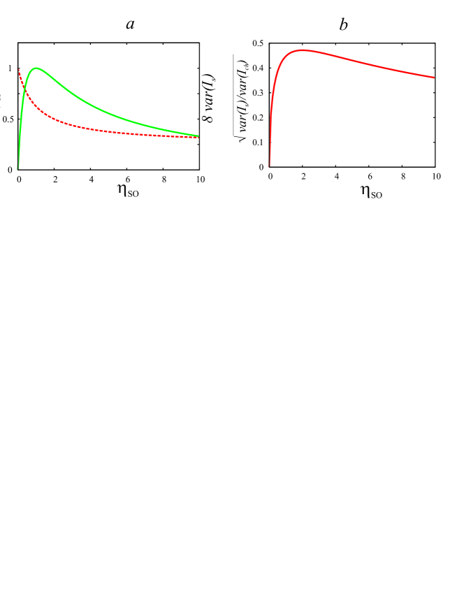
Figure 2: Tunnel connectors a. Variations of charge (dashed line) and spin currents versus the strength of spin-orbit interaction $\eta_{SO}$. The variations are normalized by the value of charge current fluctuations at $\eta_{SO}=0$. Note factor of $8$ in the scale for spin current fluctuations. b. Ratio of variations changes slowly in a wide interval of $\eta_{SO}$.

We plot in Fig. 2 the strength of spin and charge fluctuations and its ratio versus $\eta_{SO}$. Spin fluctuations reach maximum at $\eta_{SO}\approx 0.75$. The ratio of the fluctuations reaches maximum at $\eta_{SO}\approx 1.5$ and falls off very slowly upon increasing $\eta_{0}$. The polarization of the fluctuating current in maximum is about 50 %.

7 Ballistic Connectors

Let us turn to the analysis of purely ballistic connectors ($T_{i}=1$). As in previous Section, we arrange transport channels into connectors and label them with $i$. The fluctuations are contributed by LDF and GDF mechanisms. Again we assume $V_{i}\ll E_{Th}$. We integrate the non-equilibrium factor $F$ over energies to obtain (apart from $e^{2}$ factor) a strikingly simple expression:

$$\tilde{F}=\sum_{i}I_{i}\tilde{V}_{i}/G_{\Sigma}$$ (34)

where $\tilde{V}_{i}$ is the voltage drop at the corresponding connector. The non-equilibrium factor is thus proportional to the total energy dissipation in the system.

The factor determines the strength of the spin current fluctuations. From the general answer (26) we obtain the contribution of LDF mechanism:

$$\langle\!\langle I^{\alpha}_{i}I^{\beta}_{j}\rangle\!\rangle=\delta_{\alpha\beta}=\frac{G^{2}_{Q}}{e^{2}G_{\Sigma}}\tilde{F}\left(G_{i}\delta_{ij}-\frac{G_{i}G_{j}}{G_{\Sigma}(1+\eta_{SO})^{2}}\right)\frac{\eta_{SO}(2+\eta_{SO})}{(1+\eta_{SO})^{2}}$$ (35)

We can explicitly see that the fluctuations are local ( with the reservation made above). It is instructive to give the expression for the charge current fluctuations:

$$\langle\!\langle I_{i}I_{j}\rangle\!\rangle=\delta_{\alpha\beta}=\tilde{F}\left(G_{i}\delta_{ij}-\frac{G_{i}G_{j}}{G_{\Sigma}}\right)\left(1+\frac{3}{(1+\eta_{SO})^{2}}\right)$$ (36)

The contribution of the GPF mechanism reads:

$$\langle\!\langle I^{\alpha}_{i}I^{\beta}_{j}\rangle\!\rangle=\delta_{\alpha\beta}\tilde{F}\frac{G_{i}G_{j}}{8G_{\Sigma}(1+\eta_{SO})^{2}}\frac{\eta^{2}_{SO}(2+\eta_{SO})}{(1+\eta_{SO})^{2}}$$ (37)

In distinction from the tunnel junction system, there is a fluctuation of the full current to/from the system, $I^{\alpha}_{F}\equiv\sum_{i}I^{\alpha}_{i}$. It simply reads

$$\langle\!\langle I^{\alpha}_{i}I^{\beta}_{j}\rangle\!\rangle=\frac{G_{Q}^{2}}{e^{2}}\tilde{F}\frac{\eta_{SO}(2+\eta_{SO})}{(1+\eta_{SO})^{2}}$$ (38)

where we sum up the contributions of both mechanisms.

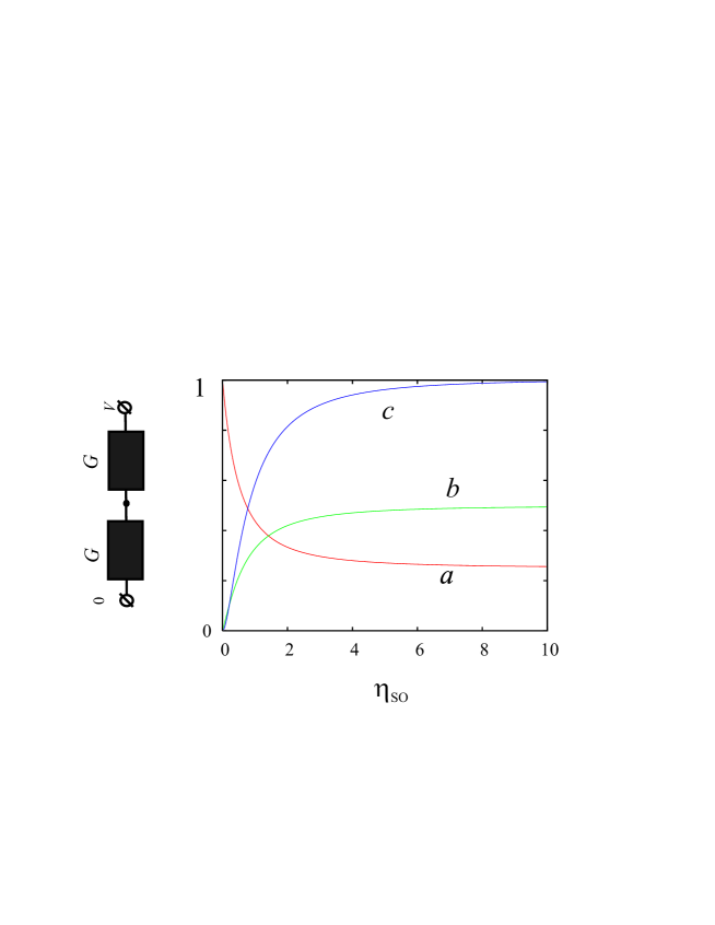
Figure 3: Ballistic connectors. We concentrate on a simple circuit with identical connectors (on the left). We plot variances of charge current (a), spin current in a connector(b), and full spin current to/from the node. The variances are normalized on the charge current variance at $\eta_{SO}$.

We plot in Fig. 3 the fluctuations of electric current, full and transport spin current for a simple system of two connectors with equal conductances.

8 Conclusions

To conclude, we have studied the mesoscopic fluctuations of spin currents for generic model of a single-node, multi-terminal nanostructure. Spin-orbit interaction is characterized by a single parameter $\eta_{SO}$ which is the ratio of the dwell time $\hbar/E_{Th}$ in the node to spin relaxation rate $\tau_{SO}$. At moderate values of this parameter, the scale of spin current fluctuations is the same as that of charge current fluctuations.

We have found that the spin current fluctuations are contributed by four distinct mechanisms: Fluctuations of polarization or distribution, both can be either local or global. Local mechanisms survive in the limit of strong spin-orbit interaction. If all connectors are of tunnel nature, only GPF works. For purely ballistic connectors, LDF and GDF contribute. We present simple formulas valid for tunnel and ballistic connectors and some quantitative results.

References

References

- [1] Žutić I, Fabian J and Das Sarma S 2004 Rev. Mod. Phys 76 323
- [2] Brataas A, Bauer GEW, and Kelly PJ 2006 Phys. Rep. 427 157
- [3] Jedema FJ, Filip AT, and van Wees BJ 2001 Nature 410 345; Schmidt G, Ferrand D, Molenkamp LW, Filip AT, and van Wees BJ 2000 Phys. Rev. B 62 R4790
- [4] Lorenzo AD and Nazarov YV 2005 Phys. Rev. Lett. 94 210601
- [5] Di Lorenzo A and Nazarov YV 2004 Phys. Rev. Lett. 93 046601
- [6] Brataas A, Nazarov YV, Bauer GEW 2000 Phys. Rev. Lett. 84 2481
- [7] Levitov LS, Nazarov YV, Eliashberg GM 1985 Zh. Eksp. Teor. Fiz. 88 229
- [8] Nazarov YV 1985 Fiz. Tv. Tela 27 1753
- [9] Kiselev AA and Kim KW 2001 Appl. Phys. Lett. 78 775
- [10] Pareek TP 2004 Phys. Rev. Lett. 92 076601
- [11] Yamamoto M, Ohtsuki T, and Kramer B 2005 Phys. Rev. B 72 115321
- [12] Altshuler BL 1985 JETP Lett. 41 648
- [13] Kramer B, Dittmer K, Debald S, Ohe J, Cavaliere F, and Sassetti M 2004 Mat. Sci.-Poland 22 445
- [14] Ren W, Qiao ZH , Wang J , Sun QF , and Guo H 2006 Phys. Rev. Lett. 97 066603
- [15] Nazarov YV 1990 JETP Lett. 51 426
- [16] Zyuzin AY and Serota RA 1992 Phys. Rev. B 45 12094
- [17] Nazarov YV 1999 Superlattices and Microstructures 25 1221
- [18] Campagnano G and Nazarov YV 2006 Phys. Rev. B 74 125307
- [19] Beenakker CWJ 1997 Rev. Mod. Phys. 69 731
- [20] Brouwer PW and Beenakker CWJ 1996 J. Math. Phys. 37 4904
- [21] Larkin AI and Khmelnitskii DE 1986 Zh. Eksp. Theor. Phys. 91 1815
- [22] Feigel’man MV, Larkin AI, and Skvortsov MA 2000 Phys. Rev. B 61 12361
- [23] Nazarov YV and Bagrets DA 2002 Phys. Rev. Lett. 88 196801