RF Shimming Pulses For Ex-Situ NMR Spectroscopy and
Imaging Using B1 Inhomogeneities

Abstract

I describe a method for generating “shim pulses” for NMR spectroscopy and imaging (MRI) by taking advantage of the inherent inhomogeneity in the static and radiofrequency (RF) fields of a one-sided NMR system. The RF inhomogeneity here is assumed, without loss of generality, to be a linear gradient. General polynomials in the spatial variables can be generated using $x$, $y$ and $z$ RF gradients using trains of hard pulses which result in linear combinations of monomials $xy$, $y^{2}$, $xz$ etc., and any desired scalings of these monomials. The basic shim pulse is constructed using small tip angle approximations.

I Introduction

“Shim pulses” have been proposed by Topgaard and Pines bib:topgaard_shimpulses using pairs of adiabatic pulses in combination with gradient modulations. Shim pulses for spectroscopy are meant to be used intermittently during stroboscopic FID readout; they work by correcting the phase of spins as function of spatial position while leaving the chemical shift evolution intact. Classical Hahn echo refocusing pulses are obviously inadequate since they would refocus the chemical shift as well, removing all spectral information.

For imaging purposes, shim pulses can be used to impart the correct phase at the center of k-space acquisition. The main challenges to designing shim pulses are: 1) keeping the pulse as short as possible so that large spectral widths can be used, 2) finding the best way to impart a large enough phase modulation given the limited available gradient strength during this short amount of time.

The adiabatic pulses of Topgaard are generally too long for many applications and this limits the performance of many experiments. For example, a 10 ms delay between consecutively collected samples results in a maximum spectral width of 100 Hz, and readouts of several points lead to significant $T_{2}$ relaxation.

Here, we exploit the idea that in an ex-situ NMR environment (e.g. with a single-sided NMR magnet configuration), the static field is intrinsically inhomogeneous and so is the radiofrequency (RF) field due to the nature of single-sided magnet and coil designs. It thus makes sense to think of schemes that take advantage of the inherent RF inhomogeneity, available at no additional cost, to correct for the negative effects of static field inhomogeneities.

I present a method which uses trains of hard pulses generated by inhomogeneous RF fields. It is based on the approach of Meriles et al. bib:pines_exsitu_science in the sense that hard pulses are used. However, we explicitly construct the desired polynomials. In the limit of small flip angles, these rotations commute and combine to create any desired polynomial in the spatial variables $x$, $y$ and $z$. The calculations presented herein demonstrate the ability of RF gradients to generate $z$-rotation shim pulses or excitation pulses.

II Theory

Consider the following product of four rotations:

$$e^{X}e^{Y}e^{-X}e^{-Y}=e^{[X,Y]+\dots}$$ (1)

where the dots mean “higher order terms”. In what follows, we drop these higher order terms from the notation.

We observe that if $X$ contains the spin operator $I_{x}$ and $Y$ contains $I_{y}$, the commutator $[X,Y]$ will contain $I_{z}$. This principle allows us to generate a rotation about the $z$ axis. Moreover, the product of $X$ and $Y$ in this commutator allows us to generate polynomials in the coefficients of $X$ and $Y$.

We consider therefore rotation operators of the form:

$$X_{i}=g_{i}x_{i}I_{x},\qquad Y_{j}=h_{j}y_{j}I_{y}$$ (2)

where $x_{i}$ and $y_{i}$ refer to any of the spatial variables $x$, $y$ or $z$. The commutator of $X_{j}$ and $Y_{j}$ is:

$$[X_{j},Y_{j}]=ig_{j}h_{j}x_{j}y_{j}I_{z}$$ (3)

and allows us to generate any of the following gradient terms in the monomials $x^{2}$, $y^{2}$, $z^{2}$, $xy$, $yz$ or $xz$ by picking $x_{j}$ and $y_{j}$ appropriately. Moreover, we may pick the product $g_{j}h_{j}$ to produce any desired scaling (rotation angle).

II.1 Second order shim pulse

We may combine $N$ successive groups of 4 pulses back to back to generate any linear combinations of $N$ monomials as follows:

$$\prod_{j=1}^{N}\underbrace{e^{X_{j}}e^{Y_{j}}e^{-X_{j}}e^{-Y_{j}}}_{\mbox{one monomial}}=\prod_{j=1}^{N}e^{[X_{j},Y_{j}]}=e^{iI_{z}\sum_{j=1}^{N}g_{j}h_{j}x_{j}y_{j}}$$ (4)

We will call this type of pulse a second order shim pulse (because it contains the product $x_{j}y_{j}$ of spatial variables) and denote the basic unit $e^{X_{j}}e^{Y_{j}}e^{-X_{j}}e^{-Y_{j}}$ as $S_{2}(X_{j},Y_{j})$.

While this $S_{2}$ pulse creates an $I_{z}$ rotation, it is ideal for use in stroboscopic pulse train experiments, where the phase of freely evolving spins is periodically corrected. The $S_{2}$ pulse can be converted into an excitation pulse using the following method: the $S_{2}$ pulse is sandwiched on the left by a $(\pi/2)_{y}$ on the left and $(\pi/2)^{-y}$ on the right. This has the effect of rotating $I_{z}$ into $I_{x}$, which can then serve as an excitation pulse. If multiple subunits of $S_{2}$ are used, the sandwiching need only be applied to the combined group of pulses. We note that the $(\pi/2)$ pulse should be applied using a homogeneous RF field or using composite pulses that compensate for the spatial inhomogeneity of the RF field.

II.2 Third order shim pulse

A third order shim pulse can be generated from the following sequence:

$$S_{2}(X,Y)e^{Z}\overline{S_{2}(X,Y)}e^{-Z}=e^{[[X,Y],Z]}\equiv S_{3}(X,Y,Z)$$ (5)

This double commutator is unable to generate an $I_{z}$ rotation if the building blocks are the operators $I_{x}$ and $I_{y}$. In this case, the $S_{3}$ pulse subunit generates an $I_{x}$ or $I_{y}$ rotation which can serve as excitation pulse.

To get an $I_{z}$ rotation pulse, the following modification to $S_{3}$ can be used: an $I_{x}$ rotation can be converted into an $I_{z}$ rotation using a $\pi/2$ rotation about $I_{y}$. Therefore, sandwiching the $S_{3}$ pulse, by $(\pi/2)_{y}$ on the left and $(\pi/2)^{-y}$ on the right converts it to an $I_{z}$ rotation. We note that the $(\pi/2)$ pulse should be applied using a homogeneous RF field or using composite pulses that compensate for the spatial inhomogeneity of the RF field.

II.3 Fourth order shim pulse

Generalizing these ideas, we may create a fourth order shim pulse can using the following sequence:

$$S_{3}(X,Y,Z)e^{W}S_{3}(X,Y,Z)e^{-W}=\\ e^{[[[X,Y],Z],W]}\equiv S_{4}(X,Y,Z,W)$$ (6)

This sequence of commutators can generate an $I_{z}$ rotation, for example, as follows:

$$[[[I_{x},I_{y}],I_{x}],I_{x}]=-iI_{z}$$ (7)

II.4 Higher order shim pulses

A fifth order shim pulse is given by:

$$S_{4}(X,Y,Z,W)e^{U}\overline{X,Y,Z,W}e^{-U}=\\ e^{[[[[X,Y],Z],W],U]}\\ \equiv S_{5}(X,Y,Z,W,U)$$ (8)

whereas a sixth order shim pulse is the sequence:

$$S_{5}(X,Y,Z,W,U)e^{V}\overline{S_{5}(X,Y,Z,W,U)}e^{-V}=\\ e^{[[[[[X,Y],Z],W],U],V]}\\ \equiv S_{6}(X,Y,Z,W,U,V)$$ (9)

This latter pulse generates an $I_{z}$ rotation, for example, as follows:

$$[[[[[I_{x},I_{y}],I_{x}],I_{x}],I_{x}],I_{x}]=-iI_{z}$$ (10)

This process of can be generalized to any $n$th order monomial of the form $x_{j}^{a}y_{j}^{b}$ where $a+b=n$. By concatenating any number of monomial units, we may generate any linear combinations of them, by choosing the RF pulse amplitudes to match the desired scalings of each monomial. This results in an arbitrary polynomial shim pulse.

We note that the higher the order of the mononomial term, the higher the error in the first order approximation to the rotation will be. For example, a monomial such as $x^{2}$ grows rapidly with increasing distance $x$ from the origin. Therefore, the errors grow larger close the sample edges. One possible solution to this problem is to repeat the $S_{2}$ sequence many times for smaller flip angles. The error is then reduced to any desired order provided the flip angles are made small enough. In the following section, I present results that illustrate this refinement approach.

A second possible approach would be to take a basic sequence such as $S_{2}$, repeat it a few times, and use optimal control algorithms (such as GRAPE) to find the proper spatial variables, spin operators and their relative phases in order to generate a propagator with far fewer errors in the spatial and spin operator orders. The free parameters which could be used in an optimal control optimization include pulse phase, gradient direction ($x$, $y$ or $z$) and pulse amplitude. Another method would be to use the inverse scattering transform to solve for the RF waveform given the desired excitation profile. These methods will not be discussed here.

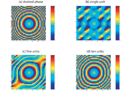
Figure 1: Simulation of a second order $x^{2}+y^{2}$ shim pulse: (a) the desired or “target” phase profile, (b) attempt at the shim pulse using a single unit of $S_{2}(X,Y)$, (c) five units and (d) ten units.

III The Refinement Method

Figure 1 shows simulations of a second order shim pulse $x^{2}+y^{2}$. Figure 1(a) shows the ideal or “target” phase profile in the $xy$ plane. The pulse unit required to generate this kind of shim pulse is

$$S_{2}(X_{1},Y_{1})S_{2}(X_{1},Y_{1})= e^{xI_{x}}e^{xI_{y}}e^{-xI_{x}}e^{-xI_{y}}$$

$$\times e^{yI_{x}}e^{yI_{y}}e^{-yI_{x}}e^{-yI_{y}}$$

$$= e^{iI_{z}(x^{2}+y^{2})}$$ (11)

This basic unit is the $N=2$ case. It requires a total of 8 hard pulses. The phase obtained from a single unit of this shim pulse is shown in Figure 1(b). We see that the pulse performs well at the origin but suffers from extreme distortions at large values of $x^{2}+y^{2}$. This pulse can be concatenated into five “smaller’ (weaker amplitude) but otherwise identical RF pulses, as shown in Figure 1(c) with a slight improvement near the center.

The ten units version of this pulse is shown in Figure 1(d) and reproduces well the desired (ideal) phase pattern of Figure 1(a). This pulse contains a total of $8\times 10=80$ hard pulses. If each hard pulses is 10 $\mu$s long, the total length of this pulse would be 800 $\mu$s. A 800 $\mu$s shim pulse is already an improvement by an order of magnitude over the Topgaard adiabatic pulses.

In practice, the total duration of each hard pulse depends on the available maximum $B_{1}$ amplitude. When considering the time-optimality of this shim pulse, only the pulse area for each hard pulse matters (duration $\times$ amplitude). Thus, in order to halve the total duration of the shim pulse, we require the doubling of $B_{1}$.

IV Conclusion

The basic idea of using RF gradients to generate arbitrary order shim pulses works, as shown in the previous simulations and theoretical expressions. Two basic errors arise in these analytical expressions: for the generation of an $I_{z}$ shim pulse, the presence of $I_{x}$ and $I_{y}$ which “contaminate” a desired $I_{z}$ rotation, and the actual coefficient of $I_{z}$ contains not only the desired monomial but monomials which are higher order in the spatial variables. A similar argument applies to $I_{x}$ or $I_{y}$ pulses for excitation purposes.

It is likely that the performance of such pulses could be improved by optimal control methods, where the spatial variables $x_{j}$, $y_{j}$, $z_{j}$ pulse amplitudes $g_{j},h_{j}$ and pulse phases $I_{x}$ vs. $I_{y}$ (or intermediate phases) are used as optimization parameters during the search. This requires that some fidelity measure for the propagator is used that minimizes the errors in the “outer parts” of the spatial variables, where the pulse errors are largest. By allowing arbitrary choices of the spatial variables and their coefficient in the optimization algorithm, it could be possible to eliminate the higher order spatial terms (monomials) in $I_{z}$ via cancellations (negative terms could possibly cancel positive terms). By allowing the phase of the RF pulse elements to vary, additional desirable elements such as robustness to offsets, and elimination of spurious spin operator terms $I_{x}$, $I_{y}$ from the propagator of a desired $I_{z}$ rotation would be possible.

References

- [1] D. Topgaard, R.W. Martin, D. Sakellariou, C.A. Meriles, and A. Pines. Shim pulses for NMR spectroscopy and imaging. Proc. Natl. Acad. Sci. USA, 101:17576–17581, 2004.
- [2] C.A. Meriles, D. Sakellariou, H. Heise, A.J. Moulé, and A. Pines. Approach to high-resolution ex situ NMR spectroscopy. Science, 293:82–85, 2002.