Entanglement and Timing-Based Mechanisms in the Coherent Control of Scattering Processes

Abstract

The coherent control of scattering processes is considered, with electron impact dissociation of H${}_{2}^{+}$ used as an example. The physical mechanism underlying coherently controlled stationary state scattering is exposed by analyzing a control scenario that relies on previously established entanglement requirements between the scattering partners. Specifically, initial state entanglement assures that all collisions in the scattering volume yield the desirable scattering configuration. Scattering is controlled by preparing the particular internal state wave function that leads to the favored collisional configuration in the collision volume. This insight allows coherent control to be extended to the case of time-dependent scattering. Specifically, we identify reactive scattering scenarios using incident wave packets of translational motion where coherent control is operational and initial state entanglement is unnecessary. Both the stationary and time-dependent scenarios incorporate extended coherence features, making them physically distinct. From a theoretical point of view, this work represents a large step forward in the qualitative understanding of coherently controlled reactive scattering. From an experimental viewpoint, it offers an alternative to entanglement-based control schemes. However, both methods present significant challenges to existing experimental technologies.

I Introduction

Coherent control CCbook is an approach to controlling quantum processes where the phase coherence between different quantum states is explicitly used in order to enhance or suppress a desired outcome of a given quantum event through interference effects. In the case of scattering, control over the product cross sections has been shown to be achievable by creating a coherent superposition of incident scattering states LabConditions ; degen . Unlike the coherent control of unimolecular processes, which has been established both theoretically and experimentally CCbook , applications of coherent control to collisions is only in its infancy. Hence it is important, at this early stage, to clarify and reinforce its essential principles, as well as to identify and develop qualitative pictures and insights applicable to a wide class of scattering problems, including the all-important case of reactive scattering.

Previous studies LabConditions ; degen focusing on crossed beam scenarios at fixed total energy have identified necessary requirements for the coherent control of scattering events. In these stationary state scenarios, incident states consisting of coherent superpositions of internal and translational motions were considered. In general, due to the conservation of center-of-mass momentum and of energy during the collision, initial state entanglement between the internal and center-of-mass states of the incident beams was found to be required. Here entanglement refers to the non-separability of the initial wave function when written in terms of the lab frame coordinates of the incident scattering particles. This requirement presents a considerable challenge to experimental implementation of the coherent control of scattering processes, and is partially responsible for the lack of coherent control scattering experiments thus far. The need for initial state entanglement in stationary state scenarios can be removed if superpositions of degenerate internal states are useddegen . However, reliance upon such entanglement-exempt systems greatly restricts the choice of possible situations that can be used in the coherent control scenario.

Although the formalism leading to conditions for the coherent control of stationary state scattering is clearLabConditions , the associated qualitative insight into the role of initial state entanglement is lacking. In this paper, we expose the universal configuration-based mechanism that lies at the core of such coherently controlled scattering LabConditions . Although our results are applicable to all scattering processes, we focus below on the most challenging case of reactive scattering. In particular, by analyzing the generic fixed total energy control scenarios where entangled interfering pathways are required, it is found that entanglement between the two incident beams ensures that all collisions within the scattering volume occur at a single favorable configuration of internal states. Further, controlling the relative phases of the entangled interfering pathways is shown to shape the internal state wave function that participates in the scattering event.

Having identified this general mechanism, we extend this thinking to the time-dependent scattering regime, allowing us to introduce an alternate approach to controlled reactive scattering that uses non-entangled wave packets of translational motion. This approach relies on the observation that translational wave packets have a finite size, so that there is a finite volume of overlap in both space and time, defined by the scattering beams, wherein the collisions occur. If the internal configuration does not have time to change as the molecules move across the collision region, then a desired configuration can be established and maintained during the collision time, allowing coherent control of reactive scattering despite the absence of initial state entanglement. This method of control relies on the presence of temporal correlations in the incident state (the collisions need to be precisely timed relative to the internal motion) as opposed to initial state entanglement.

As a result of this work we have exposed the underlying qualitative mechanism for coherently controlled scattering and developed it within both stationary and non-stationary frameworks. Each approach has its own challenges in experimental implementation, and each has its individual benefits. For example, the time-dependent wave packet version is perhaps conceptually and intuitively simpler, while the stationary state entangled version is not limited to scenarios with restricted collision volumes in space and/or time.

In the molecular scattering literature, it is frequently the case that one uses time-dependent (i.e. wave-packet) methods to calculate essentially time-independent scattering properties Zhang , such as energy-resolved cross sections. That usage of wave packets is intended solely as a computational convenience, and the same scattering results could have been computed using fully time-independent methods. We emphasize that, by contrast, the stationary and time-dependent scattering control schemes that we discuss do not simply refer to two different computational methodologies used to calculate the same physical scattering scenario. Rather, the stationary and time-dependent control scenarios embody physically distinct extended coherence properties: one requires initial state entanglement while the other requires temporal correlations between the incident wave packet.

Similarly, the time dependent scheme introduced below does not just consist of simple shaping of a translational wavefunction incident on a single state of a target molecule. Such a scenario would be akin to the previously studied 2PACC scenario2pacc which we have recently shownmichaelvlado does not involve any aspect of quantum interference, and is hence not coherently controlled collision dynamics. Rather, as shown below, our time dependent approach invokes specific interference effects to affect the product cross sections.

As a working example to illustrate these ideas, we consider electron impact dissociation of H${}_{2}^{+}$, where the total dissociation cross section and energy spectrum of the ejected protons are the observables to be controlled. However, it should be stressed that the arguments and conclusions to follow are completely general and could have been illustrated using any scattering example. Similarly, none of our results relies on the use of the Born approximation that is invoked below. However, the specific example of e-H${}_{2}^{+}$ collisions is focused upon since it is of central interest to the emerging field of strong field attosecond physics CorkumRecollision , where laser-induced ionization followed by electron recollision with the parent ion lie at the core of many processes.

The paper is organized as follows: Section II provides a reformulation of controlled stationary state scattering which affords insight into the origin of conditions for control, and Sect. III displays the underlying mechanism for control via computations on electron impact dissociation of H${}_{2}^{+}$. The extension of these qualitative control insights to the case of time-dependent scattering is discussed in Sect. III.2. Section IV provides a summary.

II Formalism

II.1 General stationary state scattering considerations

Typical crossed molecular beam experiments are well described by stationary state scattering theory at fixed total energy. Consider then a few general results from stationary state scattering theory. Within the $S$-matrix formalism Child ; Taylor the transition probability from the initial $|{\bf a}\rangle$ to final $|{\bf b}\rangle$ state is

$$S_{\bf ab}=\left\langle{\bf b}\left|e^{-i\int_{-\infty}^{\infty}{\widehat{H}}dt}\right|{\bf a}\right\rangle=\delta_{\bf ab}-iT_{\bf ab},$$ (1)

where ${\widehat{H}}$ is the scattering Hamiltonian, $T_{\bf ab}$ is the transition matrix, and $\delta_{\bf ab}$ represents the unscattered component. Note that all equations are written in atomic units $\hbar=m_{e}=e=1$. The $T$-matrix elements have the form

$$T_{\bf ab}=2\pi\>\delta(E_{\bf b}-E_{\bf a})\>\delta({\bf K}_{\bf a}-{\bf K}_{\bf b})\>t_{\bf ab},$$ (2)

where $E_{\bf a}$ and $E_{\bf b}$ are the energies of the initial and final states, ${\bf K}_{\bf a}$ and ${\bf K}_{\bf b}$ are the center-of-mass momentum of these states. The $t_{\bf ab}$ are the “on-shell” $T$-matrix elements, and depend only on the relative momentum, ${\bf k}_{\bf a}$ and ${\bf k}_{\bf b}$, and the internal quantum numbers, denoted ${\bf a}^{\prime}$ and ${\bf b}^{\prime}$, of the incident and outgoing states. Physically, the two $\delta$-functions in Eq. (2) enforce conservation of energy and of total center-of-mass momentum.

When the scattering pair is launched in a single eigenstate $|{\bf a}\rangle$ of the reactant system, the differential cross section is

$$\frac{d\sigma_{{\bf b^{\prime}}}({\bf a})}{d\Omega}=(2\pi)^{4}\Big{|}(1/|{\bf k}_{{\bf a}}|)t_{\bf ab}\Big{|}^{2},$$ (3)

where ${\bf K}_{\bf b}={\bf K}_{\bf a}$, the magnitude of the outgoing relative momentum is

$$|{\bf k}_{\bf b}|=\sqrt{2(|{\bf k}_{\bf a}|^{2}/2+E_{{\bf a}^{\prime}}-E_{{\bf b}^{\prime}})},$$ (4)

and $\Omega$ is the 3D angle of the vector ${\bf k}_{\bf b}$. The total cross section for a particular reactive arrangement channel $n$ is then found by summing over all internal states belonging to $n$, and integrating over the solid angle $\Omega$,

$$\sigma^{(n)}({\bf a})=\sum_{{\bf b}^{\prime}\in n}\int\frac{d\sigma_{{\bf b}^{\prime}}({\bf a})}{d\Omega}d\Omega.$$ (5)

Since the on-shell transition matrix elements naturally depend on the initial state $|{\bf a}\rangle$, one way to enhance/suppress a desired reactive cross section is to use a single incident state $|{\bf a}\rangle$, and vary it until the particular incident state is found that achieves this goal. This method is termed passive single-state control.

Experimentally creating a single incident scattering eigenstate is not always an easy task. Often, internal degrees of freedom of the scattering pairs are in a thermal distribution of quantum states. In this situation, cross sections can be controlled to some degree by varying, for example, the internal temperature of the particles leading to a temperature-dependent cross section

$$\sigma^{(n)}(T)=\frac{1}{Z}\sum e^{-E_{{\bf a}^{\prime}}/kT}\sigma^{(n)}({\bf a}^{\prime}),$$ (6)

where $Z$ is the partition function. Varying the temperature then changes the distribution of states that participate in the collision, and hence offers control. The thermal case can, of course, be identified as a particular case of scattering from an incoherent initial distribution, which in general leads to cross sections of the form

$$\sigma^{(n)}(F)=\left(\sum_{\bf a}F({\bf a})\sigma^{(n)}({\bf a})\right)\Bigg{/}\left(\sum_{\bf a}F({\bf a})\right),$$ (7)

where $F({\bf a})$ defines the incoherent distribution of incident states. Since all incoherent distributions provide averages over the single-state cross-sections, one can never achieve greater controllability using incoherent distributions than that achievable in single-state scattering. However, the use of coherent superpositions of incident eigenstates, instead of incoherent distributions, provides an opportunity to do better than the single-state scenario.

II.2 Superposition states and coherent control

The results in Sect. II.1 may be extended by considering scattering from an initial superposition state, either of fixed energy (and hence stationary) or of varying energy content (and hence non-stationary). The full differential cross section for scattering from the coherent initial superposition

$$|\Psi_{0}\rangle=\sum_{{\bf a}^{\prime}}\iint dk_{\bf a}dK_{\bf a}\>C({\bf a}^{\prime},k_{\bf a},K_{\bf a})\>|{\bf a}^{\prime}\rangle|k_{\bf a}\rangle|K_{\bf a}\rangle$$ (8)

is

$$\frac{d\sigma_{{\bf b}^{\prime}}(\Psi_{0})}{d{\bf k}_{\bf b}dK_{\bf b}}=(2\pi)^{4}\bigg{|}\sum_{\bf a^{\prime}}(1/|k_{\bf a}|)t_{\bf ab}C({\bf a}^{\prime},k_{\bf a},K_{\bf a})\bigg{|}^{2}$$ (9)

where again $K_{\bf a}=K_{\bf b}$, and the initial relative momenta corresponding to each ${\bf k}_{\bf b}$ and ${\bf b}^{\prime}$ is now given by

$$k_{\bf a}=\sqrt{2(|{\bf k}_{\bf b}|^{2}/2+E_{{\bf b}^{\prime}}-E_{{\bf a}^{\prime}})}.$$ (10)

For simplicity, the assumption that all incident momenta lie along a single axis (i.e. the initial momenta of the two particle are antiparallel) was used to arrive at Eq. (9). However, full dimensionality is allowed in the outgoing states. Allowing for off-axis incident momenta would simply introduce addition integrals over the initial momenta to Eq. (9), but the results of the present study are otherwise unaffected. The total cross section for scattering into channel $n$ is obtained from Eq. (9) as

$$\sigma^{(n)}(\Psi_{0})=\sum_{{\bf b}^{\prime}\in n}\iint\frac{d\sigma_{{\bf b}^{\prime}}(\Psi_{0})}{d{\bf k}_{\bf b}dK_{\bf b}}d{\bf k}_{\bf b}dK_{\bf b}.$$ (11)

Within the coherent control approach, the relative phases between multiple pathways from the initial to final state are used to control the process. By controlling the relative phase of the (complex-valued) $C({\bf a}^{\prime},k_{\bf a},K_{\bf a})$ in the initial state Eq. (8), multiple coherent pathways can be created that manifest themselves as the sum over ${\bf a}^{\prime}$ in Eq. (9). From the form of the $T$-matrix [Eq. (2)], we see that all allowed transitions must conserve center-of-mass momentum and total energy. This leads immediately to the general requirement for scattering interference: the initial states contain on-shell coherence, that is, in order for two initial eigenstates to interfere, they must belong to a single shell as defined by the $\delta$-functions in the $T_{\bf ab}$-matrix. Hence, pathways in Eq.(9) exhibit on-shell coherence (since $K_{\bf a}=K_{\bf b}$, and Eq. (10) is simply a statement of energy conservation) if the initial superposition Eq. (8) contains more than one state satisfying these on-shell requirements.

In the case of field-free bimolecular scattering governed by Eq. (2), as will be evidenced below, superposition states with coherence in the lab frame translational motion of both incident particles, and at least one internal mode (minimum 3 degrees of freedom in total), is required for interference. If static or time-dependent external fields are present during the collision event then they will modify the on-shell conditions, through energy and momentum exchange with the particles, and can lead to less restrictive conditions on the required initial-state coherence.

II.3 e-H${}_{2}^{+}$ scattering

As an example of this formalism we will consider electron impact dissociation of H${}_{2}^{+}$. The Hamiltonian for this scattering problem is given by

$${\widehat{H}} = \frac{\widehat{\bf P}^{2}_{1}}{2m_{p}}+\frac{\widehat{\bf P}^{2}_{2}}{2m_{p}}+\frac{\widehat{\bf p}^{2}_{b}}{2}+\frac{\widehat{\bf p}^{2}}{2}$$

$$-\frac{1}{\big{|}\widehat{\bf R}_{1}-\widehat{\bf r}_{b}\big{|}}-\frac{1}{\big{|}\widehat{\bf R}_{2}-\widehat{\bf r}_{b}\big{|}}-\frac{1}{\big{|}\widehat{\bf R}_{1}-\widehat{\bf r}\big{|}}$$

$$-\frac{1}{\big{|}\widehat{\bf R}_{2}-\widehat{\bf r}\big{|}}+\frac{1}{\big{|}\widehat{\bf R}_{1}-\widehat{\bf R}_{2}\big{|}}+\frac{1}{\big{|}\widehat{\bf r}_{b}-\widehat{\bf r}\big{|}},$$

where the momentum/position operators with the subscripts ’1’ and ’2’ refer to the two protons, those with the ’b’ subscript refer to the bound electron, and the remain operators refer to the incident electron. In this process, an electron with momentum ${\bf p}_{i}$ is incident on an H${}_{2}^{+}$ molecule of momentum ${\bf P}_{i}$, which is in an internal vibrational and rotational state labeled by ${\bf n}$ = $(\nu,J,m_{J})$ with energy $E_{\bf n}$ on the ground electronic state $\Sigma_{g}$. All indicated momenta are in the laboratory frame. During the e-H${}_{2}^{+}$ collision, the incident electron excites the bound electron from the bonding to antibonding state, $\Sigma_{g}\rightarrow\Sigma_{u}$, through the electron-electron Coulomb interaction $\widehat{V}_{ee}$. The final state of the scattered particles consists of the scattered electron with momentum ${\bf p}_{f}$ and two protons with momentum ${\bf P}_{1}$ and ${\bf P}_{2}$, one of which carries the bound electron. For the purposes of the scattering calculation, the final state of the two protons is written in terms of the center-of-mass motion of the full H${}_{2}^{+}$ composite ${\bf P}_{f}={\bf P}_{1}+{\bf P}_{2}$ and the relative motion ${\bf P}_{r}=({\bf P}_{1}-{\bf P}_{2})/2$ corresponding to a continuum state of energy $E=|{\bf P}_{r}|^{2}/2\mu$ and angular momentum state $L$ on the $\Sigma_{u}$ surface of H${}_{2}^{+}$, where $\mu=m_{p}/2$ is the reduced mass of the molecular ion and $m_{p}$ is the mass of the proton. The $\Sigma_{u}$ continuum states asymptotically approach the free particle momentum states defined by ${\bf P}_{1}$ and ${\bf P}_{2}$ at large distances, but are distorted near the core.

The on-shell transition matrix elements can be evaluated to first order in the electron-electron interaction (first Born approximation) Kerner ; Zare ,

$$t_{\bf a^{\prime}b^{\prime}}=\left\langle\phi^{(u)}_{E,L},{\bf k}_{f}\left|\widehat{V}_{ee}\right|\phi^{(g)}_{\bf n},{\bf k}_{i}\right\rangle,$$ (13)

where the energies are given by

$$E_{\bf a} = \frac{{\bf p}_{i}^{2}}{2}+\frac{{\bf P}_{i}^{2}}{2m_{I}}+E_{\bf n},$$ (14a)

$$E_{\bf b} = \frac{{\bf p}_{f}^{2}}{2}+\frac{{\bf P}_{f}^{2}}{2m_{I}}+E,$$ (14b)

${\bf K}_{j}$ and ${\bf k}_{j}$ ($j=i,f$) are the initial and final center-of-mass and relative momenta of the e-H${}_{2}^{+}$ system

$${\bf K}_{j} = {\bf p}_{j}+{\bf P}_{j},$$ (15a)

$${\bf k}_{j} = \frac{m_{I}{\bf p}_{j}-{\bf P}_{j}}{m_{I}+1},$$ (15b)

and $m_{I}=2m_{p}$ is the mass of the ion. The electron-electron interaction matrix elements, $\left\langle\phi^{(u)}_{E,L},{\bf k}_{f}\left|\widehat{V}_{ee}\right|\phi^{(g)}_{\bf n},{\bf k}_{i}\right\rangle$, are evaluated in full-dimensionality using the LCAO approximation for the bound electron Zare as described in Appendix A. We avoid additional approximations Kerner ; Zare by using numerical wave functions for the radial molecular continuum states, with the $\Sigma_{g}$ and $\Sigma_{u}$ surfaces taken from Ref. BunkinTugov .

The full differential dissociative cross section is

$$\frac{d\sigma^{(D)}_{L}(\Psi_{0})}{dEd{\bf k}_{f}dK} = (2\pi)^{4}\left|\sum_{\bf n}(1/k_{i0})\left\langle\phi^{(u)}_{E,L},{\bf k}_{f}\left|\widehat{V}_{ee}\right|\phi^{(g)}_{\bf n},k_{i0}\right\rangle\left\langle\phi^{(g)}_{\bf n},k_{i0},K|\Psi_{0}\right\rangle\right|^{2},$$ (16)

where

$$k_{i0}=\sqrt{2\left(|{\bf k}_{f}|^{2}/2+E-E_{\bf n}\right)},$$ (17)

and the initial momenta are again assumed to be antiparallel. The cross section $d\sigma^{(D)}/dE$, dependent only on the energy of the ejected protons $E$, is calculated by integrating over the unobserved coordinates

$$\frac{d\sigma^{(D)}(\Psi_{0})}{dE}=\sum_{L=1,3,5...}\iint\frac{d\sigma^{(D)}_{L}(\Psi_{0})}{dEd{\bf k}_{f}dK}d{\bf k}_{f}dK$$ (18)

and the total yield is given by

$$\sigma^{(D)}(\Psi_{0})=\int\frac{d\sigma^{(D)}(\Psi_{0})}{dE}dE.$$ (19)

III Coherent control of reactive scattering

III.1 Stationary State Scattering: Few-state entangled superpositions

From the requirement of on-shell coherence, the simplest (in terms of number of states involved) incident superposition [Eq. (8)] that offers on-shell coherence, and hence coherent control, utilizes two different ${\bf a^{\prime}}$ states, both with the same total energy (i.e. internal plus translational energy), at the same center-of-mass momentum $K$, i.e. a state of the form:

$$|\Psi_{os}\rangle=C_{1}|{\bf a}^{\prime}_{1}\rangle|k_{1}\rangle|K\rangle+e^{i\phi}C_{2}|{\bf a}^{\prime}_{2}\rangle|k_{2}\rangle|K\rangle,$$ (20)

where $C_{1}$ and $C_{2}$ are real. The associated differential cross section is then

$$\frac{d\sigma(\Psi_{os})}{d{\bf b^{\prime}}dK} = (2\pi)^{4}\left|C_{1}(1/k_{1})t_{{\bf a}_{1}^{\prime}{\bf b}^{\prime}}+e^{i\phi}C_{2}(1/k_{2})t_{{\bf a}_{2}^{\prime}{\bf b}^{\prime}}\right|^{2}$$

$$= (2\pi)^{4}\bigg{[}|C_{1}(1/k_{1})t_{{\bf a}_{1}^{\prime}{\bf b}^{\prime}}|^{2}+|C_{2}(1/k_{2})t_{{\bf a}_{2}^{\prime}{\bf b}^{\prime}}|^{2}$$

$$+ |C_{1}(1/k_{1})t_{{\bf a}_{1}^{\prime}{\bf b}^{\prime}}||C_{2}(1/k_{2})t_{{\bf a}_{2}^{\prime}{\bf b}^{\prime}}|\cos(\varphi_{{\bf a}_{1}^{\prime},{\bf a}_{2}^{\prime}}+\phi)\bigg{]}.$$

where $\varphi_{{\bf a}_{1}^{\prime},{\bf a}_{2}^{\prime}}$ is the phase of $t^{*}_{{\bf a}_{1}^{\prime}{\bf b}^{\prime}}t_{{\bf a}_{2}^{\prime}{\bf b}^{\prime}}$. Varying the relative phase $\phi$ of the two components in Eq. (20) controls interferences in the scattered state and provides a means of controlling the scattering products. By tuning $\phi$ one can enhance or suppress the cross sections beyond the values attainable with single-state and incoherent scenarios that utilize the same states, provided that $t_{{\bf a}_{1}^{\prime}{\bf b}^{\prime}}$ and $t_{{\bf a}_{2}^{\prime}{\bf b}^{\prime}}$ are not too dissimilar.

The state $|\Psi_{os}\rangle$ is expressed above in center-of-mass and relative coordinates. In lab frame coordinates, explicitly for the example of e-H${}_{2}^{+}$ scattering, $|\Psi_{os}\rangle$ becomes

$$|\Psi_{os}\rangle=C_{1}|{\bf n}^{(1)}\rangle|P^{(1)}_{i}\rangle|p^{(1)}_{i}\rangle+C_{2}e^{i\phi}|{\bf n}^{(2)}\rangle|P^{(2)}_{i}\rangle|p^{(2)}_{i}\rangle,$$ (22)

subject to the constraints

$$P^{(1)}_{i}+p^{(1)}_{i} = P^{(2)}_{i}+p^{(2)}_{i}$$ (23a)

$$\frac{(P^{(1)}_{i})^{2}}{2m_{I}}+\frac{(p^{(1)}_{i})^{2}}{2}+E_{{\bf n}^{(1)}} = \frac{(P^{(2)}_{i})^{2}}{2m_{I}}+\frac{(p^{(2)}_{i})^{2}}{2}+E_{{\bf n}^{(2)}}.$$ (23b)

Note that, in the general case when the internal state $|{\bf n}^{(1)}\rangle$ and $|{\bf n}^{(2)}\rangle$ are not degenerate, Eq. (22) is an entangled state of translational and internal motion, as previously discussedLabConditions . For degenerate internal states, Eq. (23) permit the solution $P^{(1)}_{i}=P^{(2)}_{i}$, $p^{(1)}_{i}=p^{(2)}_{i}$, thus removing the initial state entanglement requirementdegen .

In the remainder of this section we analyze this control scenario to expose the qualitative mechanism lying at the core of the entangled stationary state control, and then use this insight to introduce a time-dependent non-entangled version of coherently controlled reactive scattering, described further in the following subsection.

An example of control using the state Eq. (22) is shown in Fig. 1. Specifically, this example superposes two molecular vibrational states with $\nu$ = 0 and 1 and with energies $E_{0}$ = -0.0973 au and $E_{1}$ = -0.0871 au, angular momentum $J=m_{J}=0$, and translational momenta $P_{i}^{(1)}$ = 0 au and $p_{i}^{(1)}$ = 4 au The momenta $P_{i}^{(2)}$ and $p_{i}^{(2)}$ are then set in accordance with Eq. (23). The weights of the two components are set equal, $C_{1}=C_{2}$. Panel (a) shows the total cross section for dissociation as $\phi$ is varied. For comparison, the two dashed lines show the cross sections for the $\nu=0$ (lower line) and $\nu=1$ (upper line) states, considered separately. Enhancement or suppression of the total cross section beyond the incoherent result is clearly evident in Fig. 1 when using the entangled coherent superposition Eq. (22). The remaining two panels show the energy resolved cross sections, $d\sigma^{(D)}/dE$, for the states $\nu=0$ and $\nu=1$ individually [panel (a)], and for the superposition states corresponding to the extrema of $\sigma^{(D)}(\phi)$, namely $\phi$ = 0 and $\pi$ [panel (b)]. A large degree of control over the proton energy spectrum is evident.

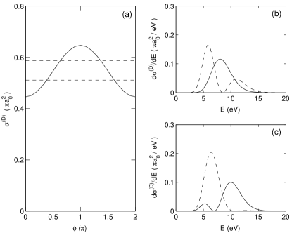
Figure 1: Control of reactive scattering using the entangled initial state Eq. (22). Panel (a) shows the dependence of the dissociation cross section $\sigma^{(D)}$ on $\phi$. The dashed lines denote $\sigma^{(D)}$ for a single component wave function using $\nu=0$ (lower line) and $\nu=1$ (upper line). Panel (b) plots the energy spectrum of the proton fragments using $\nu=0$ (solid) and $\nu=1$ (dashed). Panel (c) shows the analogous spectra when using the two-state superposition with $\phi=0$ (solid) and $\phi=\pi$ (dashed).

An important physically transparent qualitative picture of how the control arises for the entangled state can be constructed. To do so, we first note that there is ample evidence Zhang ; kernel that the exchange kernels between the reactant and product arrangements are short range. As such, the behavior of the wave function when the reactants are close to one another is particularly relevant to the reactive cross sections. For this reason, we focus below on the character of the wave function at short range.

In relative and center-of-mass momenta, the incident state is

$$|\Psi_{os}\rangle=\left[C_{1}|\nu^{(1)}\rangle|k_{i}^{(1)}\rangle+C_{2}e^{i\phi}|\nu^{(2)}\rangle|k_{i}^{(2)}\rangle\right]|K_{i}\rangle.$$ (24)

Since the center-of-mass momentum is conserved during the scattering, only the terms in the square brackets in Eq. (24) are relevant for the control dynamics. Figures 2a and 2b show the probability $P(R,x)=|\langle R,x|\Psi_{os}\rangle|^{2}$, of finding $|\Psi_{os}\rangle$ at the nuclear bond length $R$ and electron-ion separation $x$ (the conjugate of $k_{i}$). The internal states and incident momenta are the same as those used in Fig. 1; panel (a) shows results for $\phi$ = 0, while panel (b) uses $\phi=\pi$. Note that these plots show the incident states in the absence of interparticle interactions; they do not include the scattered component. The addition of the latter will change our argument quantitatively but not qualitatively. As noted above, of particular interest is the character of the internal state near the collision region, $x\approx 0$. Since $|\Psi_{os}\rangle$ is a time-independent wave function the probabilities plotted in Figs. 2a and 2b reflect the complete incident dynamics of the scattering pair. Panels (a) and (b) show that the internal vibrational wave function near $x=0$, in fact for all $x$, is controlled by $\phi$. Further, from Eq. (24), it is seen that the wave function at $x=0$ is

$$\langle R,x=0|\Psi_{os}\rangle=\left[C_{1}\langle R|\nu^{(1)}\rangle+C_{2}e^{i\phi}\langle R|\nu^{(2)}\rangle\right],$$ (25)

which, by varying $\phi$, can be shaped into structures not accessible using individual incident eigenstates. Since the cross section is strongly dependent on the internal wave function, controlling $\phi$ then allows one to control $\sigma^{(D)}$ and $d\sigma^{(D)}/dE$ by manipulating the particular internal configuration that participates in the collision. This is the qualitative mechanism lying at the core of coherently controlled reactive scattering using the entangled superposition state Eq. (22): The initial superposition state defines the structure of the internal state wave function at the point of collision and can therefore be used to tune this structure in order to optimize the reactive cross section.

In standard scattering theory one often considers scattering of incident time-independent eigenstates, and hence this observation may seem trivial. This is not the case. Had a non-entangled wave function of the form

$$|\Psi^{(ne)}_{os}\rangle = [C_{1}|{\bf n}^{(1)}\rangle+C_{2}e^{i\phi_{a}}|{\bf n}^{(2)}\rangle]$$

$$\times [C_{3}|P^{(1)}_{i}\rangle+C_{4}e^{i\phi_{b}}|P^{(2)}_{i}\rangle]$$

$$\times [C_{5}|p^{(1)}_{i}\rangle+C_{6}e^{i\phi_{c}}|p^{(2)}_{i}\rangle]$$

been used, the resultant incident state would contain 8 terms, only two of which are at the same total energy and center-of-mass momentum, namely the components in Eq. (22). From an energy domain perspective, this means that only two of the total eight terms exhibit on-shell coherence, and hence only two of the eight terms can interfere. The remaining six terms contribute incoherently to the cross sections. From a time domain perspective, only the superposition of the two on-shell components lead to a time-independent wave function. All other components, since they are at different energies, accumulate a time-dependent phase relative to the on-shell superposition. With respect to the internal configuration near the collision region, this means that the off-shell components will alternate between constructive and destructive interferences at different times, introducing a time-average over all possible phases relative to the on-shell component, and hence an average over internal configurations allowed by the populated internal states at the collision point. These time-varying interferences reduce the off-shell contribution to an effective incoherent contribution. The entanglement in the few-state superposition Eq. (22) then plays a crucial role in limiting the particular internal state wave functions that participate in the scattering events.

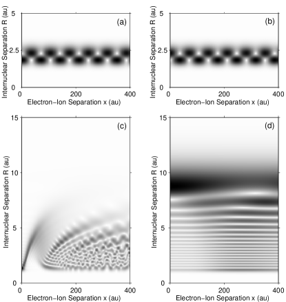
Figure 2: Plots of the probability density of relative and internal motion $P(R,x)=|\langle R,x|\Psi\rangle|^{2}$. initial state Eq. (22). Panels (a) and (b) correspond the case shown in Fig. 1 for $\phi=0$ and $\pi$ respectively. Panels (c) and (d) show incident states constructed by hand to minimize and maximize the nuclear bond length at the moment of collision, and hence minimize and maximize $\sigma^{(D)}$.

Further investigation of the e-H${}_{2}^{+}$ cross section strengthens the configuration-based qualitative mechanism described above. In particular, it is known that the electron impact dissociation cross section of H${}_{2}^{+}$ is a strongly dependent monotonic function of bond length $R$; as $\langle R\rangle$ increases, so does $\sigma^{(D)}$ Peek . Comparing the $x=0$ structure in Figs. 2a and 2b shows that the control of $\sigma^{(D)}$ follows the expected $\langle R\rangle$-dependence; the $\phi=\pi$ case has both the larger $\langle R\rangle$ and $\sigma^{(D)}$.

Using this insight, a clear extension of the two-state entangled coherent control scenario to a multi-state entangled scenario, in order to achieve better enhancement/suppression than that of Fig. 1, can be constructed. Since control here is directly linked to the average bond length at $x=0$, the superpositions that maximize/minimize the scattering cross sections are the same superposition that maximize/minimize $\langle R\rangle$ at $x=0$. For example, two superpositions (constructed by hand) that approximately achieve these goals are

$$|\Psi_{\rm max}\rangle=N_{\rm max}\left[\sum_{\nu}(-1)^{\nu}e^{-\left(\frac{\nu-18}{1.8}\right)^{2}}|\nu\rangle|k_{\nu}\rangle\right]|K\rangle$$ (27)

and

$$|\Psi_{\rm min}\rangle=N_{\rm min}\left[\sum_{\nu}e^{-\left(\frac{\nu-7}{6}\right)^{2}}|\nu\rangle|k_{\nu}\rangle\right]|K\rangle$$ (28)

where $N_{\rm max}$ and $N_{\rm min}$ are normalization constants, $k_{0}$ = 4 au, and the remaining $k_{\nu}$ are set to ensure that all components satisfy the on-shell requirement, having the same total energy and center-of-mass momentum. The summation runs over all the vibrational states $|\nu\rangle$. The corresponding $P(R,x)$ are shown in Figs. 2c and 2d. For these states, the values of $\langle R\rangle$ in the collision region are $\langle\Psi_{\rm max}|R|\Psi_{\rm max}\rangle_{x=0}=8.75$ au and $\langle\Psi_{\rm min}|R|\Psi_{\rm min}\rangle_{x=0}=1.32$ au, while the largest and smallest values possible using an incoherent initial state would correspond to those of the highest and lowest vibrational states of $H_{2}^{+}$, i.e., $\langle\nu=18|R|\nu=18\rangle_{x=0}=8.12$ au and $\langle\nu=0|R|\nu=0\rangle_{x=0}=2.05$ au The coherent superpositions $|\Psi_{\rm max}\rangle$ and $|\Psi_{\rm min}\rangle$ access values of $\langle R\rangle$ at $x=0$ beyond those accessible to any incoherent mixture of states, and hence provide more control over $\sigma^{(D)}$ than any incoherent scenario.

Note that although in the case of e-H${}_{2}^{+}$ scattering there is a clear classical explanation of the nature of the configuration that enhances control, this is need not be the case in general. Rather, given the Hamiltonian $\widehat{H}$ and the associated scattering matrix $S_{\bf ab}$, there is a well defined scattering configuration that maximizes control. When the on-shell (and hence entanglement) requirements are met for the initial superposition [Eq. (8)] then the varying the coefficients $C({\bf a}^{\prime},k_{\bf a},K_{\bf a})$ in Eq. (8) alters the stationary spatial configuration and hence alters the cross sections. The optimal choice of the $C({\bf a}^{\prime},k_{\bf a},K_{\bf a})$ then corresponds to the superposition that comes closest to the optimal stationary state configuration for scattering. Whether the optimal configuration is easily understood classically, however, depends upon the system under consideration.

III.2 Non-entangled wave-packet superpositions: Time dependent scattering

Having exposed the qualitative mechanism that underlies control resulting from stationary state, and hence entangled, initial superposition states, additional approaches to coherent control of reactive scattering that do not rely on initial state entanglement can be identified. For example, there is an alternative route to ensuring that collisions between two particles occur at a fixed phase of the internal-state motion: design time-dependent superposition states (i.e. Eq. (8) with non-degenerate states), specifically wave packets of translational motion plus superpositions of internal states, in order to localize the collision partners in space, and thereby to restrict the duration of the collision between the wave packet to less than the internal state motion (see Fig. 3a). Quantum interference manifests in this case due to the numerous energetically degenerate sets of states that occur due to the energy widths of the two incident wave packets.

The initial state used to illustrate the wave packet scenario is

$$|\Psi_{W}(t=0)\rangle=|\psi_{\nu}\rangle|\psi_{p_{i}}\rangle|\psi_{P_{i}}\rangle,$$ (29)

where

$$|\psi_{\nu}\rangle=\left[|\nu=0\rangle+e^{i\phi}|\nu=1\rangle\right]/\sqrt{2},$$ (30a)

$$|\psi_{p_{i}}\rangle=\int dp_{i}(\Delta_{p_{i}}\sqrt{\pi})^{-\frac{1}{2}}e^{-\frac{1}{2}\left(\frac{p_{i}-p_{i0}}{\Delta_{p_{i}}}\right)^{2}}|p_{i}\rangle,$$ (30b)

and

$$|\psi_{P_{i}}\rangle=\int dP_{i}(\Delta_{P_{i}}\sqrt{\pi})^{-\frac{1}{2}}e^{-\frac{1}{2}\left(\frac{P_{i}-P_{i0}}{\Delta_{P_{i}}}\right)^{2}}|P_{i}\rangle,$$ (30c)

as depicted in schematically in Fig. 3a. Note that this is not simply wavepacket scattering off of a single vibrational state. Rather, scattering is off an internal superposition of states, necessary to incorporate interference and achieve coherent control.

To get an idea of how long the collision between the two wave packets lasts, the following measure, here called the time-dependent collision probability $W_{c}(t)$, is used

$$W_{c}(t)=N\left|\left\langle\Psi(t)\left|\delta({\bf x}-{\bf y})\right|\Psi(t)\right\rangle\right|^{2}$$ (31)

where ${\bf x}$ and ${\bf y}$ are the positions of the electron and ion respectively, $|\Psi(t)\rangle$ is the incident wave function (i.e. scattered components are not included) and $N$ is a normalization constant such that $\int W_{c}(t)dt=1$. This quantity gives the probability of finding the electron and the ion at the same position in space, and hence reflects the probability of a collision occurring at time $t$. In the continuous beam scenario, as considered in the previous section, $W_{c}(t)$ is a time-independent constant. However for wave packet collisions, $W_{c}(t)$ will be a localized Gaussian-like function indicating that, in this case, collisions only occur during a select time window where the two colliding wave packets overlap in space. The duration of the wave packet collision is then defined as twice the standard deviation of $W_{c}(t)$

$$\Delta W_{c}=2\sqrt{\langle t^{2}\rangle_{W_{c}}-\langle t\rangle^{2}_{W_{c}}},$$ (32)

where $\langle\cdots\rangle_{W_{c}}$ indicates an average value where $W_{c}(t)$ is used as the distribution function.

In order to compare the wave packet scenario to the entangled state scenario, we set the mean incident momenta of Eq. (22) to $P_{i0}=0$ and $p_{i0}=4$ au, the same as used above. Using then momentum widths of $\Delta_{P_{i}}=1$ au and $\Delta_{p_{i}}=0.01$ au gives a scattering scenario where $\Delta W_{c}=0.87$ fs. Since $\Delta W_{c}$ in this case is much smaller than the vibrational period of H${}^{+}_{2}$ ($\tau_{vib}=14.9$ fs), we expect that control is possible using these parameters. Figure 3b plots the corresponding reactive cross section as $\phi$ is varied. Control is indeed present. Further, upon comparing Figs. 3b and 1a, one sees that the control using the non-entangled state Eq. (29) gives the same degree of control as the entangled state Eq. (22) confirming that the wave packet scenario offers an alternate and equivalent (in terms of the controllability of the total cross section) means of coherent control of reactive scattering, at least for reactive scattering absent of any resonances related to the relative momentum $k_{i}$. This latter point will be revisited in the following section and is at the root of possible advantages of using the entangled scenario.

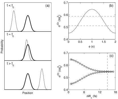
Figure 3: Control of reactive scattering using the wave packets of translational motion. Panel (a) shows schematically the wave packet scenario: controlling the internal state of the molecular ion during the finite duration of the collision allows for control. $t_{c}$ denotes the time of the collision. Panel (b) shows the degree of control using the initial Eq. (29). See the text for the specific parameters used. Panel (c) demonstrates the loss of control as the duration of the collision between the two wave packet approaches the timescale of the internal state motion. The dashed line denotes the vibrational period of H${}^{+}_{2}$, $\tau_{vib}=14.9$ fs.

The remaining panel of Fig. 3 plots the minimum and maximum values of the cross section, which correspond to $\phi$ = 0 and $\pi$, as the duration of the wave packet collision $\Delta W_{c}$ is increased. Two different methods of increasing $\Delta W_{c}$ were explored. For the first method, $\Delta p_{i}$ is gradually made smaller and smaller, which causes the spatial size of the electron wave packet to increase and thereby increases $\Delta W_{c}$. The control results using this technique, plotted against $\Delta W_{c}$, are shown in Fig. 3c using the solid curves. The second method offsets the spatial and temporal focus of the electron wave packet relative to the ion wave packet

$$|\psi_{{\bf p}_{i}}\rangle = \int dp_{i}(\Delta_{p_{i}}\sqrt{\pi})^{-\frac{1}{2}}e^{-\frac{1}{2}\left(\frac{p_{i}-p_{i0}}{\Delta_{p_{i}}}\right)^{2}}$$

$$\times e^{ip_{i}x_{d}}\>e^{-i(p_{i}^{2}/2)\tau_{d}}|p_{i}\rangle$$

where $x_{d}\equiv p_{i0}\tau_{d}$, and $\tau_{d}$ controls the focusing offset. The control results using this method are plotted in Fig. 3c with circles. In both cases, the control goes to zero as the $\Delta W_{c}$ approaches the vibrational period $\tau_{vib}$. These calculations most clearly demonstrate the configuration-based mechanism underlying the control; the controllability decreases as more internal configurations participate in the collisional events.

III.3 Entangled or Wave Packets?

Both the stationary state and non-stationary state control schemes present technological challenges. The wave packet case requires, experimentally, a collision over very short times, and therefore must be run in either a pulsed mode, or with very tightly focused molecular beams with small overlap region such that the molecules move through the collision region in a time smaller than the timescale characteristic of the dynamics of the internal superposition. The stationary state case, on the other hand, requires initial state entanglement, but can be used in a continuous beam regime and/or with arbitrarily large spatial region of overlap of the two beams. Hence, the entangled version offers arbitrarily large space-time scattering volumes while spatial restrictions exist for the wave packet version. This implies that, although the cross sections may be controlled to the same degree, the entangled version will always permit larger total yields since it came be used in conjunction with arbitrarily large volumes and incident fluxes.

A second advantage of the entangled scenario relates to the possibility of scattering resonances. The reactive cross section for e-H${}^{+}_{2}$ scattering is a rather smooth function of the incident relative momentum $k_{i}$. Hence, our sample cases thus far have implicitly considered the control of reactive scattering in the absence of sharp resonances related to the incident kinetic energy. However, reactive scattering problems of chemical interest may exhibit such resonances (e.g. Feshbach resonances). The pulsed wave packet scenario requires a broad superposition of incident momenta in order to obtain spatial localization and short-time overlaps of the two incident wave functions, while the entangled case can use as few as two incident momenta. It may very well be the case that narrow resonances can be resolved/exploited in the entangled case vlado , while averaging over the broad momentum bandwidth in the wave packet case washes out the narrow resonance features, rendering them unusable in this latter scenario.

Note that both of these aspects of initial state entanglement, the possibility to efficiently exploit narrow resonances and access arbitrarily large scattering volumes, represent non-classical aspects of controlled reactive scattering accessible via entanglement.

IV Summary

Previous work on stationary state coherent control, which provides a useful description of crossed beam experiments, was shown to require initial state entanglement between the incident translational and the internal states of the scattering partnersLabConditions . This paper has provided physical insight into the role of this requirement, generating an extension to coherent control via time-dependent wave packet scattering. Specifically, the initial state entanglement was shown to assure that all collisions occur at a fixed configuration of the internal state motion. This qualitative insight then allows for the introduction of a coherent control scenario in time-dependent scattering. Control in the latter regime is possible if the duration of the wave packet collision is much smaller than the characteristic timescales of motion of the superposition of internal states.

The mechanism of fixed-configuration scattering underlying coherent control of reactive scattering can be extended to all scattering scenarios. A sample extension to scattering off surfaces is provided elsewheremichaelvlado .

Some extensions of this approach are worth noting. First, scattering studies carried out on loosely bound van der Waals complexes Wittig are distantly related to the wave packet control scenario. In these studies, a CO₂ $\cdot$ HBr complex was used as an oriented precursor to study the CO₂ + H reaction, where photodissociation of HBr launched the H toward the CO₂. These experiments are examples of the selection of well defined angular wave packets of the scattering partners. However, for active control of reactive scattering in these systems, one would also need to tune the particular angular wave packets that participate, as opposed to selecting the single orientation defined by the initial van der Waals complex. This could perhaps be accomplished by selectively exciting rotational states of the CO₂ and/or HBr prior to the initiation of the reaction.

Second, although not explored in this paper, both the entangled and wave packet scenarios explored herein could be used instead to completely characterize the scattering matrix $S_{\bf ab}$ with phases, in analogy with methods of Quantum Process Tomography QPT . In short, having selective control over the input internal state, in addition to the usual control over the input translational momenta, would allow one to measure enough projections of the scattering operators, through measurements of the scattering cross sections for different internal superpositions, to allow for an accurate reconstruction of the complex $S$-matrix.

V Acknowledgments

This work was support through a Discovery Grant from the National Science and Engineering Research Council (NSERC) of Canada.

Appendix A Electron Impact Matrix Elements

For both the strong field and field-free scenario, the transition matrix elements $\langle\Psi_{out}|\widehat{V}_{ee}|\Psi_{in}\rangle$ are required. In calculating these values, we use the LCAO approximation for the bound electronKerner ; Zare . Specifically, using a basis of definite energy and angular momentum for the final state of the internuclear coordinate ${\bf R}$ and restricting the initial H${}_{2}^{+}$ to zero angular momentum gives

$$\langle\phi^{(u)}_{E,L},{\bf k}_{f}|\widehat{V}_{ee}|\phi^{(g)}_{\bf n},{\bf k}_{i}\rangle=i^{L}\sqrt{(2L+1)}{\cal R}(L,\nu,E,\tilde{k}),$$ (34)

where $\tilde{\bf k}\equiv{\bf k}_{f}-{\bf k}_{i}$, $\tilde{k}=|\tilde{\bf k}|$, and

$${\cal R}(L,\nu,E,\Delta k)=\frac{16}{\pi^{2}}\frac{1}{{\tilde{k}}^{2}[4+{\tilde{k}}^{2}]^{2}}\times$$

$$\int N^{(+)}(R)N^{(-)}(R)\chi_{E,J}(R)j_{L}({\tilde{k}}R/2)\chi_{\nu}(R)dR.$$ (35)

The z-axis of the angular states lies along $\Delta{\bf k}$, and only the $m_{L}=0$ sub-levels along this axis have non-zero amplitude. The $N^{(\pm)}(R)$ are normalization factors arising from the LCAO wave functions of the bound electron and are given by

$$N^{(\pm)}(R)=\left[2\pm 2e^{-R}(1+R+R^{2}/3)\right]^{-1/2}.$$ (36)

The $\chi_{\nu}(R)$ are the bound radial eigenstates on the $\Sigma_{g}$ surface

$$\left[-\frac{1}{2\mu}\frac{\partial^{2}}{\partial R^{2}}+V_{\Sigma_{g}}(R)-E_{\nu}\right]\chi_{\nu}(R)=0$$ (37)

while the $\chi_{E,L}(R)$ are the continuum radial eigenstates on $\Sigma_{u}$

$$\left[-\frac{1}{2\mu}\frac{\partial^{2}}{\partial R^{2}}+V_{\Sigma_{u}}(R)+\frac{L(L+1)}{2\mu R^{2}}-E\right]\chi_{E,L}(R)=0.$$ (38)

The $V_{\Sigma_{g}}(R)$ and $V_{\Sigma_{u}}(R)$ surfaces are taken from Bunkin and Tugov BunkinTugov . $V_{\Sigma_{g}}(R)$ is written in Morse oscillator form, and hence analytical Morse oscillator states are used for $\chi_{\nu}(R)$, while the $\chi_{E,L}(R)$ are integrated numerically and normalized such that (see Child, Appendix A Child )

$$\int_{0}^{\infty}\chi^{*}_{E^{\prime},L}(R)\chi_{E,L}(R)dR=\delta(E-E^{\prime}).$$ (39)

References

- (1) M. Shapiro and P. Brumer, Principles of the Quantum Control of Molecular Processes (John Wiley & Sons, Hoboken, NJ, 2003); S.A. Rice and M. Zhao, Optical Control of Molecular Dynamics, (John Wiley & Sons, Hoboken, N.J. 2000)
- (2) M. Shapiro and P. Brumer, Phys. Rev. Lett. 77, 2574 (1996); A. Abrashkevich, M. Shapiro, and P. Brumer, Phys. Rev. Lett. 81, 3789 (1998); 82, 3002(E) (1999); Chem. Phys. 267, 81 (2001); P. Brumer, A. Abrashkevich, and M. Shapiro, Discuss. Faraday Soc. 113, 291 (1999); J. B. Gong, M. Shapiro and P. Brumer, J. Chem. Phys. 118, 2626 (2003); See also Ref. vlado .
- (3) P. Brumer, K. Bergmann and M. Shapiro, J. Chem. Phys. 113, 2053 (2000); C.A. Arango, M. Shapiro, and P. Brumer, Phys. Rev. Lett. 97, 193202 (2006); C.A. Arango, M. Shapiro, and P. Brumer, J. Chem. Phys. 125, 094315 (2006).
- (4) J.Z.H. Zhang, Theory and Application of Quantum Molecular Dynamics (World Scientific Publishing Co., Singapore, 1999).
- (5) S. Jorgensen and R. Kosloff, Surf. Sci. 528, 156 (2003); J. Chem. Phys 119, 149 (2003); Phys. Rev. A 70, 015602 (2004).
- (6) M. Spanner, V. Zeman and P. Brumer (to be published)
- (7) H. Niikura, F. Légaré, R. Hasbani, A.D. Bandrauk, M.Yu. Ivanov, D.M. Villeneuve and P.B. Corkum, Nature (London) 417, 917 (2002); H. Niikura, F. Légaré, R. Hasbani, M.Yu. Ivanov, D.M. Villeneuve and P.B. Corkum, Nature (London) 421, 826 (2003).
- (8) M.S. Child, Molecular Collision Theory (Academic Press, London, UK, 1974).
- (9) J.R. Taylor, Scattering Theory: The Quantum Theory on Nonrelativistic Collisions (John Wiley & Sons, New York, NY, 1972).
- (10) E.H. Kerner, Phys. Rev. 92, 1441 (1953).
- (11) R.N. Zare, J. Chem. Phys. 47, 204 (1967).
- (12) For models reliant on this local behavior see, e.g., U. Halavee and M. Shapiro, J. Chem. Phys. 64, 2826 (1976); J.K.C. Wong and P. Brumer, Chem. Phys. Lett. 68, 517 (1979)
- (13) F.V. Bunkin and I.I. Tugov, Phys. Rev. A 8, 601 (1973).
- (14) J.M. Peek, Phys. Rev. 134, A877 (1964).
- (15) G. Radhakrishnan, S. Buelow, and C. Wittig, J. Chem. Phys. 84, 727 (1985); S. Buelow, M. Noble, G. Radhakrishnan, H. Reisler, C. Wittig, and G. Hancock, J. Phys. Chem. 90, 1015 (1986).
- (16) V. Zeman, M. Shapiro, and P. Brumer, Phys. Rev. Lett. 92, 133204 (2004).
- (17) I.L. Chuang and M.A. Nielsen, J. Mod. Opt. 44, 2455 (1997); R. Gutzeit, S. Wallentowitz, and W. Vogel, Phys. Rev. A 61, 062105 (2000).