Coherent Control and Entanglement in the Attosecond Electron Recollision Dissociation of D${}_{2}^{+}$

Abstract

We examine the attosecond electron recollision dissociation of D${}_{2}^{+}$ recently demonstrated experimentally [H. Niikura et al., Nature (London) 421, 826 (2003)] from a coherent control perspective. In this process, a strong laser field incident on D₂ ionizes an electron, accelerates the electron in the laser field to eV energies, and then drives the electron to recollide with the parent ion, causing D${}_{2}^{+}$ dissociation. A number of results are demonstrated. First, a full dimensional Strong Field Approximation (SFA) model is constructed and shown to be in agreement with the original experiment. This is then used to rigorously demonstrate that the experiment is an example of coherent pump-dump control. Second, extensions to bichromatic coherent control are proposed by considering dissociative recollision of molecules prepared in a coherent superposition of vibrational states. Third, by comparing the results to similar scenarios involving field-free attosecond scattering of independently prepared D${}_{2}^{+}$ and electron wave packets, recollision dissociation is shown to provide an example of wave-packet coherent control of reactive scattering. Fourth, this analysis makes clear that it is the temporal correlations between the continuum electron and D${}_{2}^{+}$ wave packet, and not entanglement, that are crucial for the sub-femtosecond probing resolution demonstrated in the experiment. This result clarifies some misconceptions regarding the importance of entanglement in the recollision probing of D${}_{2}^{+}$. Finally, signatures of entanglement between the recollision electron and the atomic fragments, detectable via coincidence measurements, are identified.

I Introduction

Laser-based quantum control techniques can be loosely characterized by two general control ideologies: scenarios based in a time-domain perspective, such as pump-dump PumpDump control, and scenarios based in the energy domain such as multi-path interference BrumerShapiro and STIRAP STIRAP control. The quantum control of reactive scattering also fits these paradigms, where examples of multi-path interference (energy-domain) BrumerScattering and wave packet (time-domain) Me schemes for coherently controlled chemical reactivity can be found. In this article, the coherent control of attosecond electron recollision dissociation is studied using both pump-dump and multi-slit interference schemes, and we find that this process offers the first experimental demonstration of wave-packet coherent control of reactive scattering Me .

The recollision experiment that is the focus of this paper proceeds as follows. Using femtosecond lasers of intensities around $10^{14}-10^{15}$ W/cm², one ionizes an atom or molecule near a peak of the instantaneous electric field, accelerating the liberated electron in the laser field, and causing the electron to recollide with the parent ion Plasma . The ionization/recollision process occurs in less than one cycle of the laser field, and repeats every cycle when the peak electric field is large enough to cause significant ionization. For Ti:sapphire laser systems (800 nm) typical of recollision experiments, one optical period is 2.6 fs and the recollision of the continuum electron wave packet with the core lasts about 500 asec. A number of processes can occur upon recollision. The continuum electron can, for example, recombine with the ion while emitting its excess energy as a burst of XUV radiation HHG , or scatter elastically thereby taking a sub-femtosecond electron diffraction image of the ion Diffraction . Alternatively, as studied here, the molecule can undergo recollision-induced dissociation

$${\rm D}_{2}\longrightarrow{\rm D}_{2}^{+}+{\rm e}^{-}\longrightarrow{\rm D}+{\rm D}^{+}+{\rm e}^{-},$$

where the strong field ionizes D₂ in the first step. In the second step, the continuum electron excites the bound electron from the $\Sigma_{g}$ bonding state to the $\Sigma_{u}$ antibonding state thereby dissociating the molecule. This process has been demonstrated experimentally, and used to probe the vibrational motion of the D${}_{2}^{+}$ nuclear wave packet following the initial ionization of D₂ on sub-femtosecond time scales CorkumRecollision .

Here, we consider the dissociative recollision process from a coherent control perspective. First, a full dimensional quantum model, based on the Strong Field Approximation (SFA), is constructed. The model is then validated by successfully simulating the experiment, which is shown to be an example of pump-dump control, consistent with a perspective long-held by the experimental NRC group foot1 . Second, the scenario is extended to bichromatic coherent control using an initial superposition of D₂ vibrational states. Considerable control is demonstrated, motivating future experimental studies. Third, field-free scattering of D${}_{2}^{+}$ and e^- wave packets is studied in order to connect the observed control of dissociative recollision with the recently constructed theory of wave-packet coherent control of reactive scattering Me . Fourth, the role of entanglement, previously suggested to be connected to the vibrational probing scenario CorkumRecollision ; Entangle1 ; EntangleMarkus , is investigated. Specifically, by comparing the vibrational probing scenario to similar scenarios using field-free non-entangled scattering states we demonstrate that it is the temporal correlations between the scattering wave packets, and not entanglement, that allow for probing and control in dissociative recollision. Nevertheless, entanglement is still present, and we conclude the paper by identifying its signatures, detectable in coincidence measurements.

For coherent control, these results are of interest because they identify new experimentally accessible examples of both bichromatic control and wave-packet control of reactive scattering. For strong field recollision, these results are important because they clarify the role of entanglement in recollision-based probing techniques CorkumRecollision , and motivate new strong field recollision control experiments.

II Methodology

II.1 Strong Field Recollision in SFA

The SFA, a well-known method in strong field physics Reiss , is here developed for the dissociative recollision scenario. We utilize the SFA in the length gauge, and work in the single active electron approximation in that only the action of the laser on the ionized electron is considered, while the bound electron and nuclei do not interact directly with the strong field. In general, there could also be strong laser-induced coupling between the bound-electronic states leading to strong field molecular effects (e.g. bond-softening, enhanced ionization) that would affect the nuclear states. However, the dissociative recollision experiments being modeled used an angle-limited detection scheme to selectively measure D⁺ fragments coming predominantly from molecules aligned perpendicular to the laser field CorkumRecollision . Strong field molecular effects are minimized for this geometry, hence justifying their exclusion from the analysis. Note that the language below is specific to D₂, but the formalism is completely general.

The exact solution for the wave function propagation can be written in the form

$$|\Psi(t)\rangle = \widehat{U}(t,t_{0})|\Psi_{i}\rangle$$

$$= -i\int^{t}_{t_{0}}dt^{\prime}\widehat{U}(t,t^{\prime})\widehat{V}_{L}(t^{\prime})e^{-i(t^{\prime}-t_{0})\widehat{H}_{0}}|\Psi_{i}\rangle$$

$$+ e^{-i(t-t_{0})\widehat{H}_{0}}|\Psi_{i}\rangle$$

where $\widehat{H}_{0}$ is the field free Hamiltonian, $\widehat{V}_{L}(t)={\bf E}(t)\cdot\widehat{\bf r}$ is the laser-matter interaction for the electric field ${\bf E}(t)$ and the electron position $\widehat{\bf r}$. The operator $\widehat{U}(t,t_{0})$ is the full propagator, defined by

$$i\frac{\partial}{\partial t}\widehat{U}(t,t_{0})=\widehat{H}(t)\widehat{U}(t,t_{0}),\>\>\>\>\widehat{U}(t_{0},t_{0})=\widehat{I},$$ (2)

where $\widehat{H}(t)=\widehat{H}_{0}+\widehat{V}_{L}(t)$ is the system+laser Hamiltonian, and $\widehat{I}$ is the identity operator. Note that all equations are written in atomic units, $\hbar=m_{e}=e=1$. The vector potential ${\bf A}(t)$ is chosen to be

$${\bf A}(t)=-\frac{{\cal E}_{0}}{\omega}\sin(\omega t)\hat{x},$$ (3)

thus giving the electric field

$${\bf E}(t)=-\frac{\partial{\bf A}(t)}{\partial t}={\cal E}_{0}\cos(\omega t)\hat{x}.$$ (4)

The initial state $|\Psi_{i}\rangle$ is assumed to be in an eigenstate of the field-free system. The last term on the right hand side of Eq. (II.1) describes the evolution of the unperturbed component of the initial wave function. It does not contribute to the dissociative recollision channel and is therefore dropped from subsequent expressions. Expanding now the propagator $\widehat{U}(t,t^{\prime})$ appearing in Eq. (II.1) in a manner similar to Eq. (II.1), but this time expanding in the electron-electron interaction $\widehat{V}_{ee}$, yields

$$|\Psi(t)\rangle = -\int^{t}_{t_{0}}dt^{\prime}\int^{t}_{t^{\prime}}dt^{\prime\prime}\>\widehat{U}(t,t^{\prime\prime})\widehat{V}_{ee}(t^{\prime\prime})\widehat{U}(t^{\prime\prime},t^{\prime})\times$$ (5)

$$\widehat{V}_{L}(t^{\prime})e^{-i(t^{\prime}-t_{0})\widehat{H}_{0}}|\Psi_{i}\rangle,$$

where another benign term, this time related to direct ionization without recollision, was again dropped since it also does not contribute to the process under consideration.

Before applying the SFA to this exact expression for the dissociative recollision, Eq. (5) is first connected to the physical picture of ionization/propagation/recollision Plasma introduced above. In particular, consider the integrand of Eq. (5) from right to left. First, the initial state $|\Psi_{i}\rangle$ propagates field-free until the time $t^{\prime}$, when it gets a ’kick’ from the laser field $\widehat{V}_{L}(t^{\prime})$. This is followed by propagation using the full Hamiltonian for a time $(t^{\prime\prime}-t^{\prime})$ after which the wave function is affected by the electron-electron interaction $\widehat{V}_{ee}$. The wave function then propagates to the observation time $t$. Thus, the partitioning used in expanding the full propagators has yielded a propagation sequence that closely resembles the physics: The active electron first sits in the ground state until being ionized by the laser. This qualitatively matches the operators in Eq. (5) to the right of, and including, $\widehat{V}_{L}(t^{\prime})$. Following ionization, the electron then oscillates in the continuum driven by the laser field until it recollides with the core. These steps qualitatively match the effect of the operators $\widehat{V}_{ee}(t^{\prime\prime})\widehat{U}(t^{\prime\prime},t^{\prime})$.

With the formalism firmly connected to the physical picture, the SFA can now be applied. The central approximation introduced by the SFA is to neglect the interaction between the ion and the continuum electron in the intermediate propagator $\widehat{U}(t^{\prime\prime},t^{\prime})$ where the electron propagates far from the core before returning to the ion, and also in the final propagator $\widehat{U}(t,t^{\prime\prime})$. This means that once the active electron has been ionized, it acts as a completely free electron oscillating in the laser field. The only deviation from this idealization arises due to the electron-electron interaction $\widehat{V}_{ee}(t^{\prime\prime})$. From the point of view of scattering theory, this means that after ionization the continuum electron is effectively being treated by a Born-type approximation in the resulting recollision event, albeit a Born approximation dressed by the strong laser field that drives the electron recollision.

In order to carry out the SFA, complete basis sets consisting of the field-free molecular states for the nuclear component and plane waves for the active electron are inserted between the operators appearing in Eq. (5) to give

$$|\Psi(t)\rangle = -\sum_{{\bf n},{\bf n}^{\prime},J}\int dE\int^{t}_{t_{0}}dt^{\prime}\int^{t}_{t^{\prime}}dt^{\prime\prime}\int d{\bf k}\int d{\bf k}^{\prime}\int d{\bf k}^{\prime\prime}$$

$$\times \widehat{U}(t,t^{\prime\prime})|\phi^{(u)}_{E,J};{\bf k}^{\prime\prime},t^{\prime\prime}\rangle\>\langle\phi^{(u)}_{E,J};{\bf k}^{\prime\prime},t^{\prime\prime}|\widehat{V}_{ee}(t^{\prime\prime})|\phi^{(g)}_{{\bf n}^{\prime}};{\bf k}^{\prime},t^{\prime\prime}\rangle$$

$$\times \langle\phi^{(g)}_{{\bf n}^{\prime}};{\bf k}^{\prime},t^{\prime\prime}|\widehat{U}(t^{\prime\prime},t^{\prime})|\phi^{(g)}_{\bf n};{\bf k},t^{\prime}\rangle\langle\phi^{(g)}_{\bf n};{\bf k},t^{\prime}|\widehat{V}_{L}(t^{\prime})e^{-iE_{i}(t^{\prime}-t_{0})}|\Psi_{i}\rangle,$$

where $E_{i}$ is the energy of the initial state presently assumed to be an eigenstate of $\widehat{H}_{0}$ (superposition states will be considered below), $|\phi^{(g)}_{\bf n}\rangle$ are the bound nuclear states on the $\Sigma_{g}$ surface with quantum numbers ${\bf n}=(\nu,J,m)$, $|\phi^{(u)}_{E,J}\rangle$ are the continuum states with energy $E$ and and angular momentum $J$ on the $\Sigma_{u}$ surface, the electronic continuum (plane wave) states are

$$\langle{\bf r}|{\bf k},t\rangle=(2\pi)^{-(3/2)}e^{i[{\bf k}+{\bf A}(t)]\cdot{\bf r}},$$ (7)

and ${\bf k}$ is the canonical momentum of the free electron oscillating in the laser field. Within the above outlined assumptions, and after projecting onto a particular final state $|\phi^{(u)}_{E,J};{\mathbf{k}}_{f},t\rangle$, Eq. (II.1) reduces to

$$\langle\phi^{(u)}_{E,J};{\mathbf{k}}_{f},t|\Psi(t)\rangle = -\sum_{\bf n}\int^{t}_{t_{0}}dt^{\prime}\int^{t}_{t^{\prime}}dt^{\prime\prime}\int d{\mathbf{k}}$$

$$e^{-(i/2)\int^{t}_{t^{\prime\prime}}d\tau[{\mathbf{k}}_{f}+{\mathbf{A}}(\tau)]^{2}}e^{-iE(t-t^{\prime\prime})}\langle\phi^{(u)}_{E,J};{\mathbf{k}}_{f},t^{\prime\prime}|\widehat{V}_{ee}(t^{\prime\prime})|\phi^{(g)}_{\bf n};{\mathbf{k}},t^{\prime\prime}\rangle$$

$$e^{-(i/2)\int^{t^{\prime\prime}}_{t^{\prime}}d\tau[{\mathbf{k}}+{\mathbf{A}}(\tau)]^{2}}e^{-iE_{\bf n}(t^{\prime\prime}-t^{\prime})}e^{-iE_{g}(t^{\prime}-t_{0})}\langle\phi^{(g)}_{\bf n};{\mathbf{k}},t^{\prime}|\widehat{V}_{L}(t^{\prime})|\Psi_{i}\rangle,$$

where $E_{\bf n}$ is the energy of the nuclear state ${\bf n}$, and the propagation of the continuum electron was handled using the Gordon-Volkov solutions volkov

$$\langle{\mathbf{k}^{\prime},t^{\prime\prime}}|e^{-i\int^{t^{\prime\prime}}_{t^{\prime}}\widehat{H}_{V}(\tau)d\tau}|{\mathbf{k},t^{\prime}}\rangle = \langle{\mathbf{k}^{\prime},t^{\prime\prime}}|e^{-(i/2)\int^{t^{\prime\prime}}_{t^{\prime}}d\tau[{\mathbf{k}}+{\mathbf{A}}(\tau)]^{2}}|{\mathbf{k},t^{\prime\prime}}\rangle$$

$$= e^{-(i/2)\int^{t^{\prime\prime}}_{t^{\prime}}d\tau[{\mathbf{k}}+{\mathbf{A}}(\tau)]^{2}}\delta({\mathbf{k}}-{\mathbf{k}^{\prime}}),$$

which are exact solutions for a free electron oscillating in a laser field. The remaining integrals in Eq. (II.1) are evaluated using the stationary phase method, keeping the stationary points on the real time axis, yielding

$$\langle\phi^{(u)}_{E,J};{\bf k}_{f},t|\Psi(t)\rangle = -\sum_{\bf n}\sum_{j=S,L}e^{i\varphi({\bf k}_{0},t^{(j)}_{b},t^{(j)}_{c})}a_{c}(t_{c},t_{b})a_{p}(I_{p,{\bf n}},t^{(j)}_{c}-t^{(j)}_{b})a_{i}(I_{p,{\bf n}},t^{(j)}_{b})$$ (10)

$$\times \langle\phi^{(u)}_{E,J};{\bf k}_{f},t^{(j)}_{c}|\widehat{V}_{ee}(t^{(j)}_{c})|\phi^{(g)}_{\bf n};{\mathbf{k}}_{0},t^{(j)}_{c}\rangle\langle\phi^{(g)}_{\bf n};{\mathbf{k}}_{0},t^{(j)}_{b}|\widehat{V}_{L}(t^{(j)}_{b})|\Psi_{i}\rangle,$$

where

$$\varphi({\bf k}_{0},t_{b},t_{c})=-\frac{1}{2}\int^{t}_{t_{c}}d\tau[{\bf k}_{f}+{\bf A}(\tau)]^{2}-E(t-t_{c})-\frac{1}{2}\int^{t_{c}}_{t_{b}}d\tau[{\bf k}_{0}+{\bf A}(\tau)]^{2}-E_{\bf n}(t_{c}-t_{b})-E_{i}(t_{b}-t_{0}),$$ (11)

$$a_{c}(t_{c},t_{b})=e^{i\pi/4}(2\pi)^{1/2}\left|-{\bf E}(t_{c})[{\bf k}_{f}+{\bf A}(t_{b})]+{\bf E}(t_{b})[{\bf A}(t_{b})-{\bf A}(t_{c})]\frac{\partial t_{b}}{\partial t_{c}}+I_{p,{\bf n}}\frac{\partial^{2}t_{b}}{\partial t^{2}_{c}}\right|^{-\frac{1}{2}}$$ (12)

$$a_{p}(I_{p,{\bf n}},t_{c}-t_{b})=e^{-i3\pi/4}\left[\frac{2\pi}{|t_{c}-t_{b}|}\right]^{3/2}$$ (13)

$$a_{i}(I_{p,{\bf n}},t_{b})=\sqrt{\pi}\left[\frac{2}{I_{p,{\bf n}}\left|{\mathbf{E}}(t_{b})\right|^{2}}\right]^{1/4}\exp\left[-\frac{1}{3}\frac{(2I_{p,{\bf n}})^{3/2}}{\left|{\mathbf{E}}(t_{b})\right|}\right],$$ (14)

the state-to-state ionization potentials are $I_{p,{\bf n}}=E_{\bf n}-E_{i}$, the stationary phase points for the time of birth ($t_{b}$), time of collision ($t_{c}$), and momentum at birth (${\bf k}_{0}$) are given by

$${\bf k}_{0}=-{\bf A}(t_{b}) = \frac{{\cal E}_{0}}{\omega}\sin(\omega t_{b})\hat{x}$$ (15a)

$$\omega*(t_{c}-t_{b})*\sin(\omega t_{b}) = \cos(\omega t_{b})-\cos(\omega t_{c})$$ (15b)

$$\frac{1}{2}\left|{\bf k}_{f}-\frac{{\cal E}_{0}}{\omega}\sin(\omega t_{c})\hat{\bf z}\right|^{2} = \frac{1}{2}\frac{{\cal E}^{2}_{0}}{\omega^{2}}\left[\sin(\omega t_{b})-\sin(\omega t_{c})\right]^{2}-D_{E,{\bf n}}-I_{p,{\bf n}}\frac{\partial t_{b}}{\partial t_{c}}$$ (15c)

and $D_{E,{\bf n}}=E-E_{\bf n}$ is the state-dependent dissociation energy. The derivatives of $t_{b}$ with respect to $t_{c}$ are defined through Eq. (15b). For each ${\bf k}_{f}$, Eqs. (15) admit two solutions, the long (L) and short (S) trajectories, where $t^{(S)}_{c}-t^{(S)}_{b}<t^{(L)}_{c}-t^{(L)}_{b}$. The sum over $j$ in Eq. (10) accounts for these two solutions.

In principle, Eq. (10) is the final stationary phase SFA amplitude for the dissociative recollision process. However, some additional simplifications relevant to the present work are in order. First, note that while the amplitude Eq. (10) correctly captures much of the essential physics of recollision problems, such as the qualitative dependence of the final yields on laser frequency and intensity, it typically underestimates absolute yields by 1 to 2 orders of magnitude. This is due to the neglect the Coulomb potential during the ionization step. However, methods are available to correct the ionization rates, on sub-cycle time scales, by adding the Coulomb potential in some approximate way Coulomb . Second, $a_{c}(t_{c},t_{b})$ in Eq. (10) has divergences. These divergences are artificial in the sense that the stationary phase method is simply not valid at these points. Rather, one should use the uniform approximation to treat these regions. When treated correctly, $a_{c}(t_{c},t_{b})$ is a slowly-varying prefactor (as a function of the final state parameters) to the amplitude Eq. (10) and affects little but the absolute yield. Since the present study is focused on building a novel perspective of this process based upon ideas in coherent control, we choose to avoid additional computational complications, and simply drop the divergent term, recognize that the absolute value is nonquantitative and accept that this model correctly captures the dependence of the yields on the laser and initial state parameters, but gives incorrect absolute yields. Similarly, sub-cycle corrections to the ionization rate are not included. Finally, dividing Eq. (15c) by the maximum value of the vector potential ${\cal E}_{0}/\omega$ shows that the term containing $\partial t_{b}/\partial t_{c}$ is proportional to $I_{p}/(2U_{p})=\gamma^{2}$, where $\gamma$ is the Keldysh parameter Keldysh . In the tunneling ionization regime, $\gamma$ is assumed to be a small parameter, and thus the $\partial t_{b}/\partial t_{c}$ term in Eq. (15c) can be neglected. In the calculations present below, this term was neglected. However, it was checked that the results did not change, at the level of detail considered in this work, when this term was used.

Further simplifications can be made to the ionization matrix elements using Eq. (15a)

$$\langle\phi^{(g)}_{\bf n};{\mathbf{k}}_{0},t_{b}|\widehat{V}_{L}(t_{b})|\Psi_{i}\rangle=\langle\phi^{(g)}_{\bf n};-{\bf A}(t_{b}),t_{b}|\widehat{V}_{L}(t_{b})|\Psi_{i}\rangle.$$ (16)

For all $t_{b}$, the final continuum wave is $\langle{\bf r}|(-{\bf A}(t_{b})),t_{b}\rangle=(2\pi)^{-(3/2)}e^{i[0]\cdot{\bf r}}=constant$ [see Eq. (7)]. Neglecting also angular excitation of the nuclei (rotational time scales are much longer than the current time scales of interest), the ionization matrix element becomes

$$\langle\phi^{(g)}_{\bf n};{\mathbf{k}}_{0},t_{b}|\widehat{V}_{L}(t_{b})|\Psi_{i}\rangle\propto\langle\phi^{(g)}_{\bf n}|\phi^{(i)}_{\bf n}\rangle\cos(t_{b})$$ (17)

where $|\phi^{(i)}_{\bf n}\rangle$ are the nuclear states of the D₂ molecule and $|\phi^{(g)}_{\bf n}\rangle$ are the nuclear state of the D${}_{2}^{+}$ ion. The overlap $\langle\phi^{(g)}_{\bf n}|\phi^{(i)}_{\bf n}\rangle$ can be recognized as Franck-Condon factors modulating the ionization step.

With these last considerations taken into account, Eq. (10) becomes

$$\langle\phi^{(u)}_{E,J};{\bf k}_{f},t|\Psi(t)\rangle \propto -\sum_{\bf n}\sum_{j=S,L}e^{i\varphi({\bf k}_{0},t^{(j)}_{b},t^{(j)}_{c})}a_{p}(I_{p,{\bf n}},t^{(j)}_{c}-t^{(j)}_{b})a_{i}(I_{p,{\bf n}},t^{(j)}_{b})$$

$$\times \cos(t^{(j)}_{b})\langle\phi^{(u)}_{E,J};{\bf k}_{f}|\widehat{V}_{ee}|\phi_{\bf n};-{\mathbf{A}}(t^{(j)}_{b})\rangle\langle\phi^{(g)}_{\bf n}|\phi^{(i)}_{\bf n}\rangle$$

$$\equiv \langle\phi^{(u)}_{E,J};{\bf k}_{f}|\widehat{S}_{DR}|\Psi_{i}\rangle,$$

where $\widehat{S}_{DR}$, defined by Eq. (II.1) is the approximate dissociative recollision scattering operator, and the (now extraneous) time-dependence of the electronic plane wave basis was dropped. The D⁺ kinetic energy spectrum $W(E)$ is found by integrating over the final scattering electron and angular momentum states:

$$W(E)=\sum_{J=1,3,5...}\int d{\bf k}_{f}\left|\langle\phi^{(u)}_{E,J};{\bf k}_{f}|\widehat{S}_{DR}|\Psi_{i}\rangle\right|^{2}.$$ (19)

The equivalent expression when starting with an initial superposition of D₂ states $\sum_{i}C_{i}|\Psi_{i}\rangle$ is

$$W(E)=\sum_{J=1,3,5...}\int d{\bf k}_{f}\left|\sum_{i}C_{i}\langle\phi^{(u)}_{E,J};{\bf k}_{f}|\widehat{S}_{DR}|\Psi_{i}\rangle\right|^{2}.$$ (20)

Of interest is also the total yield defined as

$$W_{T}=\int W(E)dE.$$ (21)

Interfering pathways that can be used for coherent control can be seen in Eqs. (II.1) and (20). The sum over ${\bf n}$ in Eq. (II.1), that is, the vibrational motion of the nuclei between the moments of ionization and recollision, offers a means of pump-dump control, and also provides the opportunity to probe the vibrational motion of the nuclear wave packet excited to the $\Sigma_{u}$ state following ionization, the focus of the experiment CorkumRecollision . The pump-dump perspective is modeled and discussed in Sec. III.1, the results of which are in excellent agreement with the experiment, thereby confirming the validity of the SFA model. The sum over $i$ in Eq. (20) provides a means of control through preparation of an initial vibrational superposition state before the strong field is applied. This control is similar in spirit to traditional bichromatic control schemes, and is explored in Sec. III.2. There are also interferences arising from the so-called long and short trajectories [sum over $j$ in Eq. (II.1)]. However, these interferences lead to rapid oscillations of the final yield as a function of ${\bf k}_{f}$, and average to zero once the yields are integrated over ${\bf k}_{f}$.

Note that in this formulation the momentum ${\bf k}$, referred to as the free electron momentum, is in reality the relative momentum of the ion and the free electron, and that the center-of-mass momentum was assumed to be zero. In typical strong field scenarios, this subtlety is irrelevant. However, it is important to stress this point in the present study since the field-free scattering formalism, presented in the following section, will make use of both the lab frame coordinates of the electron and ion as well as the relative and center-of-mass coordinate.

II.2 Field-Free Wave-Packet Scattering

Consider then scattering in the absence of an external field. We work within the $S$-matrix formalism Child ; Taylor

$$S_{\bf ab}=\left\langle{\bf b}\left|e^{-i\int_{-\infty}^{\infty}{\widehat{H}}dt}\right|{\bf a}\right\rangle=\delta_{\bf ab}-iT_{\bf ab}$$ (22)

to calculate the transitions from the initial state $|{\bf a}\rangle=|\phi^{(g)}_{\bf n};{\bf p}_{i};{\bf P}_{i}\rangle$ to final state $|{\bf b}\rangle=|\phi^{(u)}_{E,J};{\bf p}_{f};{\bf P}_{f}\rangle$, where ${\bf p}_{i}$ (${\bf p}_{f}$) is the initial (final) momentum of the scattering electron, and ${\bf P}_{i}$ (${\bf P}_{f}$) is the initial (final) momentum of the ion, both in the laboratory frame. Within the Born approximation, the transition matrix elements $T_{\bf ab}$ to first order in the electron-electron interaction are given by

$$T_{\bf ab} = \int dt^{\prime}\left\langle{\bf a}\left|e^{-i\int_{t^{\prime}}^{\infty}{\widehat{H}}_{\bf a}dt}\widehat{V}_{ee}e^{-i\int^{t^{\prime}}_{-\infty}{\widehat{H}}_{\bf b}dt}\right|{\bf b}\right\rangle$$

$$= (2\pi)\delta(E_{\bf b}-E_{\bf a})\>\delta({\bf K}_{f}-{\bf K}_{i})\left\langle\phi^{(u)}_{E,J};{\bf k}_{f}\left|\widehat{V}_{ee}\right|\phi^{(g)}_{\bf n};{\bf k}_{i}\right\rangle,$$

with energies

$$E_{\bf a} = \frac{{\bf p}_{i}^{2}}{2}+\frac{{\bf P}_{i}^{2}}{2m_{I}}+E_{\bf n},$$ (24a)

$$E_{\bf b} = \frac{{\bf p}_{f}^{2}}{2}+\frac{{\bf P}_{f}^{2}}{2m_{I}}+E.$$ (24b)

Here ${\bf K}_{j}$ and ${\bf k}_{j}$ ($j=i,f$) are the center-of-mass and relative momenta of the e-D${}_{2}^{+}$ system

$${\bf K}_{j} = {\bf p}_{j}+{\bf P}_{j},$$ (25a)

$${\bf k}_{j} = \frac{m_{I}{\bf p}_{j}-{\bf P}_{j}}{m_{I}+1},$$ (25b)

and $m_{I}=2m_{p}$ is the mass of the ion.

Due to the $\delta({\bf K}_{f}-{\bf K}_{i})$ term in Eq. (II.2), which represents conservation of total momentum, ${\bf K}_{f}={\bf K}_{i}\equiv{\bf K}$ is a constant of motion. The scattering problem is then solved for each ${\bf K}$ individually, after which the yields are averaged incoherently over the ${\bf K}$ distribution. First, the projection of the scattered wave function onto the final state basis is calculated as

$$|\langle\phi^{(u)}_{E,J};{\bf k}_{f};{\bf K}|\Psi_{f}\rangle|^{2} = (2\pi)^{2}\Bigg{|}\sum_{\bf n}\int d{\bf k}_{i}\delta(E_{\bf b}-E_{{\bf a}})$$

$$\times \left\langle\phi^{(u)}_{E,J};{\bf k}_{f}\left|\widehat{V}_{ee}\right|\phi^{(g)}_{\bf n};{\bf k}_{i}\right\rangle\langle\phi^{(g)}_{\bf n};{\bf k}_{i};{\bf K}|\Psi_{0}\rangle\Bigg{|}^{2}.$$

With the initial translational momenta of both the electron and ion antiparallel in the laboratory frame, as done in the following sections, Eq. (II.2) can be reduced to

$$|\langle\phi^{(u)}_{E,J};{\bf k}_{f};K|\Psi_{f}\rangle|^{2} = (2\pi)^{2}\left|\sum_{\bf n}(1/k_{i0})\left\langle\phi^{(u)}_{E,J};{\bf k}_{f}\left|\widehat{V}_{ee}\right|\phi^{(g)}_{\bf n};k_{i0}\right\rangle\left\langle\phi^{(g)}_{\bf n};k_{i0};K|\Psi_{0}\right\rangle\right|^{2},$$ (27)

where

$$k_{i0}=\sqrt{2\left(|{\bf k}_{f}|^{2}/2+E-E_{\bf n}\right)}.$$ (28)

The partial yields of interest are calculated by integrating over the relevant final states

$$W_{K}(E)=\sum_{J=1,3,5...}\int d{\bf k}_{f}\left|\langle\phi^{(u)}_{E,J};{\bf k}_{f};K|\Psi_{f}\rangle\right|^{2}$$ (29)

$$W(E)=\int W_{K}(E)dK,$$ (30)

and the total yield is given by Eq.(21).

For the case of $e+D_{2}^{+}$ collisions, the electron impact matrix elements $\left\langle\phi^{(u)}_{E,J};{\bf k}_{f}\left|\widehat{V}_{ee}\right|\phi^{(g)}_{\bf n};k_{i0}\right\rangle$ are computed as previously described (Ref. Me ).

III Control Scenarios

III.1 Vibrational Probing and Pump-Dump Control

Consider first the original experiments of Niikura et al. CorkumRecollision , where the D⁺ kinetic energy spectrum was measured as a function of laser wavelength. The basic idea was to exploit the frequency-dependence of the time delay between the moment of ionization $t_{b}$ and moment of collision $t_{c}$, implicit in Eq. (15b), in order to probe the vibrational motion of the D${}_{2}^{+}$ vibrational wave packet. This vibrational probing scenario can readily be identified as a pump-dump control scenario: the ionization step pumps the nuclei to the $\Sigma_{g}$ surface while the recollision dumps the nuclear wave packet to the dissociative surface. Varying the laser frequency controls the pump-dump time delay. In fact, the vibrational probing experiments were guided by this close analogy with pump-dump control.

Figure 1 demonstrates the vibrational probing/pump-dump scenario using the SFA model. Here, and through the rest of the paper, we plot the D⁺ kinetic energy $E_{D}$ spectrum, $W_{D}(E_{D})\equiv 2W(E/2)$, using Eq. (19). The factors of 2 arise from the fact that $E$ is the relative energy shared by the D and D⁺; since the D⁺ are much heavier than the scattered electron, the center-of-mass energy of the two D⁺ is negligible and the relative energy $E$ is shared equally between the kinetic energies of the D⁺. Here $D_{2}$ was initially in its ground vibrational and rotational state, and the field strength used was ${\cal E}_{0}=0.065$ au ($I_{0}=1.4\times 10^{14}$ W/cm²). This field strength is used throughout the paper. The results were calculated for a single recollision event. Multiple recollisions would increase the absolute yield, but would not change the relative yields across the spectrum. The four panels show the D⁺ energy spectrum for the four different wavelengths (800, 1200, 1530, and 1850 nm) used in Ref. CorkumRecollision . The simulated results are in excellent agreement with the experiment CorkumRecollision , thus validating the SFA model. $W_{D}(E_{D})$ clearly depends on the wavelength, and this dependence reflects the motion of the D${}_{2}^{+}$ nuclear wave function on the $\Sigma_{g}$ surface between the moments of ionization $t_{b}$ and recollision $t_{c}$, both providing a means to probe the vibrational motion as well as offering an example of pump-dump control.

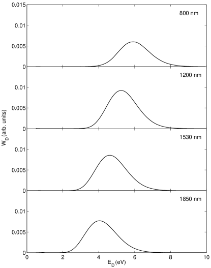
Figure 1: Pump-dump control of the dissociative recollision D⁺ spectrum. The ionization event provides the ’pump’, while recollision provides the ’dump’. The pump-dump time delay is controlled by varying the driving frequency.

III.2 Bichromatic Coherent Control

The orthodox bichromatic coherent control scenario BrumerShapiro utilizes CW lasers and involves first creating an initial superposition state and then driving the superposition to a final state where the components of the superposition can interfere. This scenario can be extended to the time domain, and to attosecond dissociative recollision, in particular by creating an initial vibrational superposition in D₂. Since the recolliding electron has a broad bandwidth (energies of recollision vary from 0 to 3.17 $U_{p}$ Plasma , where $U_{p}=({\cal E}_{0}/\omega)^{2}/4$ is the pondermotive potential), the various initially-populated vibrational states will overlap in the nuclear continuum on the antibonding surface following collisional excitation, and make possible the bichromatic control of the D⁺ energy spectrum.

This scenario is illustrated in Fig. 2 using a superposition of the $|\nu\rangle=|0\rangle$ and $|1\rangle$ vibrational states of D₂, with rotation in the ground state. The results correspond to a single recollision event and a driving field of frequency $\omega=0.0569$ au (800 nm). Panel (a) plots the final D⁺ spectra starting from $|0\rangle$ (solid) and $|1\rangle$ (dashed) individually, while panel (b) plots the spectra arising from the vibrational superpositions $|+\rangle=|0\rangle+|1\rangle$ (solid) and $|-\rangle=|0\rangle-|1\rangle$ (dashed). Panel (c) plots the total integrated D⁺ yield $W_{T}$ for the vibrational superposition state $|\phi\rangle=|0\rangle+e^{i\phi}|1\rangle$ as $\phi$ is varied. The range of control is significant. These results should strongly motivate an experimental study of bichromatic coherent control via strong field dissociative recollision: the D⁺ spectrum and total yield can be actively controlled by using phase-coherent initial states.

Figure 2: Single-cycle bichromatic control of dissociative recollision. D⁺ spectrum for initial (a) $|0\rangle$ vibrational state (solid), and initial $|1\rangle$ state (dashed); (b) initial $|0\rangle+|1\rangle$ superposition (solid) and $|0\rangle-|1\rangle$ superposition (dashed). (c) D⁺ yield from $|0\rangle+\exp(i\phi)|1\rangle$ state as a function of $\phi$.

As in the previous section, these results include only a single recollision event, thereby effectively simulating the result of driving the recollision with a single-cycle pulse. In the case of pump-dump control, adding more cycles did not change the resulting D⁺ spectrum. However, this is not the case for the bichromatic scenario. If the number of cycles is large enough so that the total time duration of the driving pulse is larger than the vibrational period of the initial superposition state, then control will disappear, since each cycle would contribute to the final D⁺ spectrum with a different phase $\phi$ due to the evolution of the vibrational eigenstates from one cycle to another. However, control can be restored in the many cycle regime by using pulses at two different frequencies,

$${\bf E}_{2}(t) = ({\cal E}_{0}/2)[\cos(\omega_{1}t)+\cos(\omega_{2}t)]\hat{x}$$ (31)

$$= {\cal E}_{0}\cos((\Delta\omega/2)t)\cos(\omega t)\hat{x},$$

where $\omega_{1}=\omega+\Delta\omega/2$, $\omega_{2}=\omega-\Delta\omega/2$, and $\Delta\omega$ is set equal to the energy difference between the two states of the initial superposition. In this case, the two frequencies will cause beats in the envelope of the long pulse that are timed to the motion of the internal state superposition (see Figs. 3a and b). Here the central frequency is set to $\omega=0.0569$ au (800 nm). Varying the relative phase of the superposition, or alternatively varying the relative phase of the two frequencies, then varies the relative timing between the internal state motion and the envelope beats, and allows one to control which phases of the vibrational superposition contribute to the recollision events.

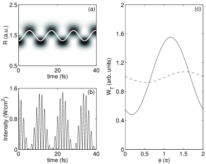
Figure 3: Many-cycle bichromatic control of dissociative recollision. (a) Density of D₂ vibrational wave function as a function of time. The undulation of the density is highlighted by the superimposed wave. (b) Incident laser intensity as a function of time for the two-color field of Eq. (31) with ${\cal E}_{0}=$, $\omega=0.0569$ au, and $\Delta\omega=0.0135$ au (c) Control of D⁺ yield as a function of $\phi$ for a monochromatic incident field of frequency $\omega$ (dashed) and the two-color field (solid).

Figure 3c shows the control, as a function $\phi$, when using a monochromatic field (dashed) and the two-color field [Eq. (31)] with $\omega=0.0596$ au and $\Delta\omega=E_{\nu=1}-E_{\nu=0}=0.0135$ au The calculations included eleven cycles of the 800 nm carrier, corresponding to two vibrational periods of the D₂ superposition. When solving the stationary phase equations for the two-color laser field, the field and vector potential were treated as pure sine waves over the half cycle,

$${\bf E}_{2}(t)\approx{\cal E}_{0}\cos((\Delta\omega/2)T_{n})\cos(\omega t)\hat{x}$$ (32)

and

$${\bf A}_{2}(t)\approx-\frac{{\cal E}_{0}}{\omega}\cos((\Delta\omega/2)T_{n})\sin(\omega t)\hat{x},$$ (33)

where the amplitude of the beat envelope $\cos((\Delta\omega/2)T_{n})$ was evaluated at the time $T_{n}$ corresponding to the peak field strength of the half cycle, defined by $\cos(\omega T_{n})=1$. For ease of comparison, both control plots were normalized so that the average yield as a function of $\phi$ is unity to compensate for the different ionization yield that depends exponentially on the instantaneous electric field strength [Eq. (14)]. As can be seen from Fig. 3c, the control with the monochromatic wave is greatly diminished for many cycles, and the control eventually reaches zero in the limit of infinite number of cycles. However, control in the case of the two-color field persists, and does not diminish further when additional cycles are added.

III.3 Coherently Controlled Reactive Scattering

An interesting question arises when one considers dissociative recollision from the perspective of coherently controlled reactive scattering. Traditional (non-control) scattering scenarios Child ; Taylor are almost all conducted in a field-free environment and use nearly monoenergetic beams. However, the present scenario necessarily involves the presence of a strong laser field and wave packets of translational momentum. Coherent control of reactive scattering in the continuous beam regime BrumerScattering is now well understood, and the wave packet extension has recently been explored Me . Although dissociative recollision clearly involves a scattering process, it is also coupled to the ionization step and the in-field propagation, and hence it is not entirely clear to what extent it can be considered as a true example of coherently controlled reactive scattering. The easiest way to address this issue is to compare the strong field recollision scenario to its $D_{2}^{+}+e^{-}$ field-free counterpart using the field-free scattering formalism presented in Sec.II.2.

The incident scattering state used to mimic the recollision event has the form

$$|\Psi_{0}\rangle=\sum_{\bf n}\int d{\bf K}d{\bf k}\>a_{\bf n}\psi({\bf k},{\bf K})|\phi^{(g)}_{\bf n},{\bf k},{\bf K}\rangle,$$ (34)

where $a_{\bf n}$ and $\psi({\bf k},{\bf K})$ are the vibrational and translational expansion coefficients respectively. In the recollision scenario, the collision between the electron and the ion lasts about 0.5 fs. For the laser intensity used above, at 800 nm, the peak recollision momentum is $p_{max}=\sqrt{2\times 3.17U_{p}}\approx 1.5$ au. This recollision wave packet can then be adequately represented in the field-free case by the following translational superposition

$$\psi({\bf k},{\bf K}) = \frac{1}{\sqrt{\pi\Delta K\Delta k}}\exp\left[-\frac{1}{2}\left(\frac{{\bf K}-{\bf K}_{0}}{\Delta K}\right)^{2}\right]$$ (35)

$$\times \exp\left[-\frac{1}{2}\left(\frac{{\bf k}-{\bf k}_{0}}{\Delta k}\right)^{2}\right],$$

with relative coordinate parameters given by $\Delta k=0.5$ au and ${\bf k}_{0}$ = 1.5 au, parameters chosen to mimic the recollision wave packet observed in the simulations of the previous sections. Since the scattering is independent of the center-of-mass parameters, any values of $\Delta K$ and ${\bf K}_{0}$ can be used. Here we set these parameters to $\Delta K=1.0$ au and ${\bf K}_{0}$ = 0 au, where ${\bf k}_{0}$ and ${\bf K}_{0}$ are parallel to each other. In order to match the D${}_{2}^{+}$ vibrational wave packet created in the strong field case, the vibrational coefficients are set to

$$a_{\bf n}\propto\langle\phi^{(g)}_{\bf n}|\phi^{(i)}_{0}\rangle\exp\left[-\frac{1}{3}\frac{(2I_{p,{\bf n}})^{3/2}}{\left|{\mathbf{E}}(t_{b})\right|}-iE_{\bf n}\tau_{d}\right]$$ (36)

where $\langle\phi^{(g)}_{\bf n}|\phi^{(i)}_{0}\rangle$ are the Franck-Condon overlaps, and the exponential mimics both the ionization amplitude [see Eq. (14)] and the time delay $\tau_{d}$ = 2.0 fs between the momentum of ionization and recollision ($\tau_{d}$ is $\sim$3/4 of the laser cycle Plasma ). This distribution of vibrational states on the $D_{2}^{+}$ surface follows from the above presented SFA theory by evaluating Eq. (II.1) after ionization but before recollision, and has been observed experimentally Urbain . Crucial from the perspective of coherent control is that the combination of a spread in population of vibrational states $|\phi^{(g)}_{\bf n}\rangle$ [Eq. (36)] and spread in incident momentum [Eq. (35)] leads to multiple energetically degenerate pathways to product states.

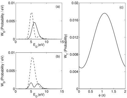
Figure 4: Field-free wave-packet coherent control of electron impact dissociation. D⁺ spectrum for initial (a) $|0\rangle$ vibrational state (solid), and initial $|1\rangle$ state (dashed); (b) initial $|0\rangle+|1\rangle$ superposition (solid) and $|0\rangle-|1\rangle$ superposition (dashed). (c) D⁺ yield from $|0\rangle+\exp(i\phi)|1\rangle$ state as a function of $\phi$.

Figure 4 plots the resulting D⁺ yields for the field-free scattering. Upon comparing panels (a) and (b) of Figs. 4 and 2, one sees that the D⁺ spectra resulting from the strong field and field-free scenarios are essentially the same. Small variations are present, for example the distributions in the field-free case are all a bit narrower than their field-free counterparts, but this is likely due to small differences between the actual recollision state and that used to mimic this state in the field-free scenario. When comparing the phase dependence of the D⁺ yields [panel (c) of Figs. 4 and 2], one sees that the general sinusoidal dependence is perfectly captured by the field-free scenario. It is therefore clear that the strong field and field-free cases behave in essentially similar ways, and hence that the dissociative recollision scenario offers an example of wave-packet control of reactive scattering.

III.4 Entanglement in Dissociative Recollision

We now address the importance of entanglement in dissociative recollision. Specifically, the literature suggests a connection between the sub-femtosecond time resolution present in the vibrational probing of the D${}^{+}_{2}$ wave packet and entanglement CorkumRecollision ; Entangle1 ; EntangleMarkus . The entanglement under consideration is that between the electron and ion after ionization and before recollision: when the D₂ is ionized, the resultant wave function is separable in relative and center-of-mass coordinates, similar to Eq. (34), but not separable in the ion and electron coordinates. The question of entanglement is also central to the coherent control of reactive scattering BrumerScattering ; Me . In that case, initial state entanglement is required for control when using superpositions of a few isolated translational plane waves BrumerScattering . Recent results show, however, that initial state entanglement is not necessary when working with specific scenarios utilizing wave packets of translational motion Me involving energetically degenerate pathways. The dissociative recollision scenario features such pathways, as noted above, and hence it is conceivable that entanglement is neither crucial for control nor for vibrational probing. This is examined below.

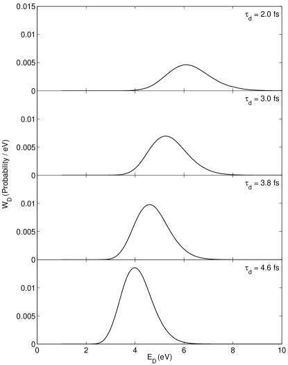
Figure 5: Non-entangled wave packet probing of vibrational motion. To be compared with Fig. 1. The $\tau_{d}$ values correspond to the pump-dump time delays for the wave lengths used in Fig.1.

To gain insight into the role of entanglement, we consider once again the analogous field-free case with independently prepared wave packets of D${}_{2}^{+}$ and e^-, but this time without entanglement present. That is, our initial state is

$$|\Psi_{0}\rangle=\sum_{\bf n}\int d{\bf P}d{\bf p}\>a_{\bf n}\psi({\bf p},{\bf P})|\phi^{(g)}_{\bf n},{\bf p},{\bf P}\rangle,$$ (37)

where

$$\psi({\bf p},{\bf P}) = \frac{1}{\sqrt{\pi\Delta P\Delta p}}\exp\left[-\frac{1}{2}\left(\frac{{\bf P}-{\bf P}_{0}}{\Delta P}\right)^{2}\right]$$ (38)

$$\times \exp\left[-\frac{1}{2}\left(\frac{{\bf p}-{\bf p}_{0}}{\Delta p}\right)^{2}\right],$$

the electronic parameters are given by $\Delta p=0.5$ au and ${\bf p}_{0}$ = 1.5 au, and the ionic parameters are $\Delta P=1.0$ au and ${\bf P}_{0}$ = 0. The $a_{\bf n}$ are the same as those used above. Recall that the ${\bf P}_{0}$ and ${\bf p}_{0}$ are momenta in the laboratory frame.

Figure 5 shows the results of mimicking the dissociative recollision probing/pump-dump scenario using the field-free non-entangled scattering scenario. The ’pump-dump time delay’ was varied by controlling $\tau_{d}$, and results for the four values of $\tau_{d}$ corresponding to the wave lengths used in the strong field pump-dump scenario are shown. Upon comparing Fig. 5 with Fig. 1, one sees that the non-entangled field-free scattering scenario does capture the vibrational motion just as well as did the strong field recollision scenario.

Note that the $W_{D}(E_{D})$ peak height increases as $\tau_{d}$ becomes larger in the field-free scenario, but the analogous peak height in the strong field case remains roughly constant. The change in total yield in the field-free case is present because the cross section for electron impact dissociation of D${}_{2}^{+}$ depends strongly on the internuclear distance; as the bond is allowed to stretch, it becomes easier to dissociate. In the strong field case, as the wave length is varied and the pump-dump time delay increases, the continuum electron wave packet spreads more in the transverse direction, thus counteracting the expected increase in the total yield as the bond length stretches.

These results directly imply that it is the temporal correlations between the incident electron wave packet and the vibrational motion of the ion that is necessary for probing/control, but entanglement is not. Further, the general agreement between Fig. 5 and Fig. 1 strengthens the argument that dissociative recollision scenarios can be considered as examples of wave-packet coherent control of reactive scattering. The theory of wave-packet coherent control of reactive scattering is discussed in detail in Ref.Me .

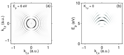
Figure 6: Signatures of entanglement in the multiparticle distributions. (a) Electron momentum spectrum, for $E_{D}$ = 6 eV, showing ATI structure. (b) Coincident D⁺ /electron spectrum, for $k_{f,y}$ = 0, showing ATI-like structures in the D⁺ kinetic energy distribution. Both spectra are taken at $k_{f,z}$=0.

Although electron-ion entanglement is not central to probing or control, the fact remains that entanglement is present. The entangled nature of the multiparticle density can be revealed through coincidence measurements, where the D⁺ kinetic energy spectrum is measured together with the recollision electron. The ionization, and subsequent recollision, certainly leads to multiparticle correlations in the outgoing state. However, to demonstrate entanglement, one must show non-separable wave function characteristics, which include correlated observables and coherence. When using a driving pulse with many cycles, the outgoing flux originating from each half cycle will interfere, hence providing a means to verify the coherence of the final wave function.

Figure 6a shows a slice through the final momentum distribution of the scattered electron taken at $E_{D}$ = 6 eV and $k_{f,z}$ = 0, calculated for a five-cycle 800 nm pulse. The ring structure, similar to the well known Above-Threshold Ionization (ATI) peaks, appear as result of the periodic nature of strong field ionization. Each half-cycle an electron wave packet is launched into the continuum. All these wave packets then interfere to produce the rings. In an energy representation each ring is separated by one unit of the photon energy. Since dissociative recollision also occurs each half cycle, similar ATI-like structures exist in the D⁺ energy spectrum, Fig.6b, again a result of interferences between the outgoing D⁺ flux originating from each half-cycle. The spectrum shown in Fig. 6b corresponds to $k_{f,y}$ = 0 and $k_{f,z}$ = 0. Unlike one-electron ATI, the ring structures resulting from dissociative recollision only appear when both the recollision electron and the D⁺ are measured in coincidence, that is, the structure exist only in such spectra. Further, since the rings are a result of quantum interference, the resulting wave function is necessarily coherent. Observation of these ATI-like rings in the coincidence spectra would then demonstrate the entanglement that is necessarily present during the dissociative recollision process.

IV Summary

We have considered the attosecond dissociative electron recollision in D₂ from the perspective of coherent control. Both pump-dump and bichromatic control schemes were demonstrated in this system. Further, by direct comparison of the strong field recollision scenario with analogous field-free cases, it was shown that this system offers an example of wave-packet coherent control of reactive scattering. By constructing and analyzing similar scenarios involving scattering of non-entangled field-free wave packets, it was shown that the electron-ion entanglement effectively plays no role in the control scenario presented herein nor in the closely related problem of recollision-based sub-femtosecond vibrational probing CorkumRecollision . Finally, detectable signatures of electron-ion entanglement in the outgoing multiparticle states, arising from temporal interferences, were identified.

V Acknowledgments

M.S. would like to thank O. Smirnova and M. Ivanov for numerous insightful discussions. Both authors acknowledge positive discussions with P. Corkum. This work was supported by the National Science and Engineering Research Council of Canada.

References

- (1) D.J. Tannor, S.A. Rice, J. Chem. Phys. 85, 5013 (1985); D.J. Tannor, R. Kosloff, S.A. Rice, J. Chem. Phys. 85, 5805 (1985).
- (2) M. Shapiro and P. Brumer, Principles of the Quantum Control of Molecular Processes, (John Wiley & Sons, New Jersey, USA, 2003).
- (3) K. Bergmann, H. Theuer, and B. W. Shore, Rev. Mod. Phys. 70, 1003 (1998).
- (4) M. Shapiro and P. Brumer, Phys. Rev. Lett. 77, 2574 (1996); A. Abrashkevich, M. Shapiro, and P. Brumer, Phys. Rev. Lett. 81, 3789 (1998); 82, 3002(E) (1999); Chem. Phys. 267, 81 (2001); P. Brumer, A. Abrashkevich, and M. Shapiro, Discuss. Faraday Soc. 113, 291 (1999).
- (5) M. Spanner and P. Brumer, Phys. Rev. A (preceding paper).
- (6) P. B. Corkum, Phys. Rev. Lett. 71, 1994 (1993).
- (7) M. Lewenstein, Ph. Balcou, M.Yu. Ivanov, Anne L’Huillier, and P.B. Corkum, Phys. Rev. A 49, 2117 (1994).
- (8) M. Lein, J.P. Marangos, and P.L. Knight, Phys. Rev. A 66, 051404 (2002); M. Spanner, O. Smirnova, P.B. Corkum, and M.Yu, Ivanov J. Phys. B: At. Mol. Opt. Phys. 37, L243 (2004); S.N. Yurchenko, S. Patchkovskii, I.V. Litvinyuk, P.B. Corkum, and G.L. Yudin, Phys. Rev. Lett. 93, 223003 (2004).
- (9) H. Niikura, F. Légaré, R. Hasbani, A.D. Bandrauk, M.Yu. Ivanov, D.M. Villeneuve and P.B. Corkum, Nature (London) 417, 917 (2002); H. Niikura, F. Légaré, R. Hasbani, M.Yu. Ivanov, D.M. Villeneuve and P.B. Corkum, Nature (London) 421, 826 (2003).
- (10) Indeed, NRC scientists such as Paul Corkum and Albert Stolow have viewed all pump-probe experiments as examples of coherent control.
- (11) J. Hu, K.-L. Han, and G.-Z. He, Phys. Rev. Lett. 95, 123001 (2005).
- (12) M. Kitzler and M. Lezius, Phys. Rev. Lett. 95, 253001 (2005).
- (13) H.R. Reiss, Prog. Quant. Electr. 16, 1 (1992).
- (14) W. Gordon, Z. Phys. 40, 117 (1926); D.V. Volkov, Z. Phys. 94, 250 (1935).
- (15) O. Smirnova, M. Spanner, and M.Yu. Ivanov, J. Phys. B: At. Mol. Opt. Phys. 39, S307 (2006).
- (16) L.V. Keldysh, Zh. eksp. teor. Fiz. 47, 1945 (1964) [English translation: Soviet Phys. JETP 20, 1307 (1965)].
- (17) M.S. Child, Molecular Collision Theory (Academic Press, London, UK, 1974).
- (18) J.R. Taylor, Scattering Theory: The Quantum Theory of Nonrelativistic Collisions (John Wiley & Sons, New York, NY, 1972).
- (19) X. Urbain, B. Fabre, E.M. Staicu-Casagrande, N. de Ruette, V.M. Andrianarijaona, J. Jureta, J.H. Posthumus, A. Saenz, E. Baldit, and C. Cornaggia, Phys. Rev. Lett. 92, 163004 (2004).
- (20) F.V. Bunkin and I.I. Tugov, Phys. Rev. A 8, 601 (1973).