Quantum theory for spatial motion of polaritons in inhomogeneous fields

Abstract

Polaritons are the collective excitations of many atoms dressed by resonant photons, which can be used to explain the slow light propagation with the mechanism of electromagnetically induced transparency. As quasi-particles, these collective excitations possess the typical feature of the matter particles, which can be reflected and deflected by the inhomogeneous medium in its spatial motion with some velocity. In this paper we develop a quantum theory to systematically describe the spatial motion of polaritons in inhomogeneous magnetic and optical fields. This theoretical approach treats these quasi-particles through an effective Schrödinger equation with anisotropic depression that the longitudinal motion is like a ultra-relativistic motion of a “slow light velocity” while the transverse motion is of non-relativity with certain effective mass. We find that, after passing through the EIT medium, the light ray bends due to the spatial-dependent profile of external field. This phenomenon explicitly demonstrates the exotic corpuscular and anisotropic property of polaritons.

I Introduction

Quasi-particles are excitations of the matter. According to modern many body theory, Elementary particles and quasi-particles are basic construction of matters. The latter are crucial for understanding many phenomena in condensed matter physics. Actually, quasi-particles can be regarded as collective excitations of many elementary particles, as well as the mixtures of different elementary excitations, whose behavior are similar to the matter particles book1 .

In atomic physics and quantum optics, some exotic phenomena can be explained by the concept of quasi-particles. For example, slow light phenomenon slow ; slow397 in electromagnetically induced transparency (EIT) Harris ; Harris82 can be explained in terms of quasi-particles - polaritons Lukin84 ; Lukin65 ; Lukin77 ; Lukin75 . EIT happens when a weak signal light field and a stronger control field are coupled to an ensemble of atoms with a $\Lambda$ energy level configuration. Under the two-photon resonance, due to the destructive interference between two interaction paths, the initially opaque resonant medium becomes transparent with respect to the probe field, and the group velocity of light is slowed down. Light then is stopped in the EIT medium because only the dark state polariton is excited. The dark state polariton is a bosonic like collective excitation, which is a mixture of a signal light field and an atomic spin wave sprl91 .

Most recently, the light deflection was observed for the EIT atomic medium in an external field with spatially inhomogeneous distribution Karpa ; Scul07 . In the experiment of Ref. Karpa , it is found that the light ray bends when a magnetic field with small gradient vertical to the propagation direction is applied to a cell with $\Lambda$-type rubidium gas. This experiment was interpreted as the Stern-Gerlach experiment of the dark polariton, thus the effective magnetic moment of the dark state polariton is observed for the first time. It demonstrates that the dark state polariton indeed behaves as a matter particle with mass, momentum and magnetic moment et al, which can be reflected, refracted, and even deflected by a gradient force. Therefore, quasi-particles show their particle nature with definite momentum and effective mass. Different from that in Ref. Karpa , the experiment of Re. Scul07 shows that a light can also been deflected by an optical driven Rb atomic vapor when the profile of the driving field is inhomogeneous. In this situation the angle of deviation is an order of magnitude larger than that in Ref. Karpa . The observed phenomenon about light deflection in such EIT media has been explained correctly according to the semi-classical theory ZDL without using the concept of dark-state polariton, which needs the quantization of light fields.

Like matter particles, quasi-particles possess the wave-particle duality, that is, quasi-particles sometimes appear to behave as particles and sometimes appear to behave as waves. Here, we are interested in the particle aspect of the dark polariton, which is an atomic collective excitation dressed by the quantized probe light. The main purpose of this paper is to systematically develop a quantum theory describing the spatial motion of polaritons in inhomogeneous magnetic and optical fields. We begin our investigation with the propagation of quasi-particles in the limits of atomic linear response, where the atomic equations are treated perturbatively. With an effective potential induced by the steady atomic response in the external spatial-dependent field, the dynamics of spatial motion of the quasi-particles is governed by the effective Schrödinger equation. The spatial motion of the quasi-particle is of anisotropic depression – the longitudinal motion is like a ultra-relativistic motion of a “slow light” while the transverse motion is of non-relativity with certain effective mass.

This paper is organized as follows: In sec. II, we present the theoretical model for a $\Lambda$-type atomic ensemble in the presence of inhomogeneous external fields, and derive the system of equations governing the spatial motion of the signal field in the atomic linear response with respect to the probe field. In Sec. III, the perturbation theory is applied to obtain the atomic motion equation which is related to the linear response to the signal field. In Sec. IV and Sec. V, the crucial idea of the EIT - the dark-state polariton is introduced as an dressed fields to describe the spatial motion of collective excitation. Afterward, the dynamics of the quasi-particle - dark polariton is discussed in the presence of an inhomogeneous magnetic field with a spatial distribution along the transverse direction. In Sec. VI, the spatial motion of the signal light in an inhomogeneous coupling field is investigated. Then we make our conclusion in Sec. VII.

II theoretical model for $\Lambda$-type atomic ensemble in external fields

We consider an ensemble of $N$ identical and noninteracting atoms, which is confined in a cell ABCD as shown in Fig. 1b. Each of the atoms is modeled by a $\Lambda$-shaped energy level configuration with internal states $\left|g\right\rangle$, $\left|s\right\rangle$ and $\left|e\right\rangle$. The transitions from the two lower states $|g\rangle$ and $|s\rangle$ to the excited state $|e\rangle$ are coupled by two optical fields, a weaker probe field and a stronger control field, as shown in the top panel of Fig. 1a. The atomic transition from $\left|g\right\rangle$ to $\left|s\right\rangle$ is forbidden by the electronic dipole coupling. The probe field carries frequency $\nu$ and the wave number $k$. It is a quantized electromagnetic field with $\sigma^{+}$ polarization. Under the rotating wave approximations, its negative frequency part of the electric field $\tilde{E}^{+}\left(\mathbf{r},t\right)$, couples the ground state $|g\rangle$ to the excited state $|e\rangle$ at resonance, in the absence of the magnetic field $B\left(\mathbf{r}\right)$. The control field has carrier frequency $\nu_{c}=\omega_{e}-\omega_{s}$ and wave number $k_{c}$. It is a classical field with $\sigma^{-}$-polarized, and couples to the upper state $|e\rangle$ and the metastable state $|s\rangle$ with Rabi frequency $\Omega\left(\mathbf{r}\right)$. After the magnetic field is applied along the $z$-direction, the internal energies of the corresponding states are shifted from their origins by magnitudes $\mu_{i}B$ with

$$\mu_{i}=m_{F}^{i}g_{F}^{i}\mu_{B},i\in\left\{g,s,e\right\}.$$ (1)

Here, $\mu_{B}$ is the Bohr magneton, $g_{F}$ is the Landé g-factor of the internal state $i$, and $m_{F}$ is the magnetic quantum number.

As shown in Fig. 1b, the probe field and the control field propagate parallel in the $z-$ direction with wave number $k$ and $k_{c}$ respectively. The Hamiltonian of this typical EIT system is given by $H=H^{(A)}+H^{(F)}+H^{(I)}$. Let us use $\tilde{\sigma}_{\mu\nu}^{j}\left(t\right)=\left|\mu\right\rangle_{j}\left\langle\nu\right|$ to denote the internal state operator of the $j$-th atom between states $\left|\mu\right\rangle$ and $\left|\nu\right\rangle$. We introduce the collective atomic operator Lukin65

$$\tilde{\sigma}_{\mu\nu}\left(r,t\right)=\frac{1}{N_{r}}\sum_{r_{j}\in N_{r}}\tilde{\sigma}_{\mu\nu}^{j}\left(t\right)\text{,}$$ (2)

which is averaged over a small but macroscopic volume containing many atoms $N_{r}=\left(N/V\right)dV\gg 1$ around position $r$. Here $N$ is the number of atoms in an interaction volume $V$. Then the Hamiltonian of the atomic part reads

$$H^{(A)}=\frac{N}{V}\sum_{j}\int d^{3}r\left(\omega_{j}-\mu_{j}B\right)\tilde{\sigma}_{jj},$$ (3)

where we have neglected the kinetic term of atoms, and $\omega_{j}$ are the corresponding energy level spacing of the internal atomic level. $H^{(F)}$ is the free Hamiltonian of the radiation field. Using the electric-dipole approximation and the rotating-wave approximation, the interaction with electromagnetic field reads Lukin84 ; Lukin65 ; Lukin77 ; Lukin75

$$H^{(I)}=-\frac{N}{V}\int d^{3}r\left[d_{eg}\tilde{\sigma}_{eg}\tilde{E}^{+}+\Omega\tilde{\sigma}_{es}e^{i\left(k_{c}z-\nu_{c}t\right)}+h.c.\right]$$ (4)

Here, $\tilde{E}^{+}$ is the negative frequency of the probe field; $\Omega\left(\mathbf{r}\right)$ is the Rabi frequency of the control field, which usually depends on the spatial coordinate through the spatial profile of driving field; $d_{eg}$ is the dipole matrix element between the states $|g\rangle$ and $|e\rangle$.

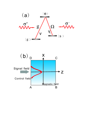
Figure 1: (Color on line) (a) Level scheme of atoms interacting with $\sigma^{+}$-polarized probe and $\sigma^{-}$-polarized probe strong fields. $\Omega$ denotes the Rabi frequency of the undepleted classical control field. (b) Configuration of the optical beams and the magnetic field inside the atomic medium.

For convenience, we describe the electric field as

$$\tilde{E}^{+}\left(r,t\right)=\sqrt{\frac{\nu}{2\varepsilon_{0}V}}E\left(r,t\right)e^{i\left(kz-\nu t\right)}$$ (5)

in the following discussion. Here $\exp\left[i\left(kz-\nu t\right)\right]$ is the carrier wave with frequency $\nu$ and wave number $k$ propagating in the $z$ direction, and $E\left(r,t\right)$ is the slow varying envelope, meaning that its spatiotemporal variation is much slower than the carrier wave length and frequency. Further we introduce the slowly varying variables for the atomic transition operators

$$\tilde{\sigma}_{eg}\left(r,t\right) =\sigma_{eg}\left(r,t\right)e^{-ikz}\text{,}$$ (6a)

$$\tilde{\sigma}_{es}\left(r,t\right) =\sigma_{es}\left(r,t\right)e^{-ik_{c}z}\text{.}$$ (6b)

In the rotating reference frame, the dynamics of this system is described by the interaction Hamiltonian

$$H_{I} =-\frac{N}{V}\int d^{3}r[\sum_{j}\mu_{j}B\sigma_{jj}$$ (7)

$$+\left(g\sigma_{eg}E+\Omega\sigma_{es}+h.c.\right)]\text{,}$$

where the atom-field coupling constant $g$ is defined as

$$g=d_{eg}\sqrt{\frac{\nu}{2\varepsilon_{0}V}}.$$ (8)

Before we study the EIT features of this system in detail, let us first stand in the point of view of light to investigate the propagation effects of pulses in an atomic medium. It is well-known that, when atoms are subjected to an electric field, the applied field displaces the positive charges and the negative charges in atoms from their usual positions. This small movement that positive charges in one direction and negative ones in the other will result in collective induced electric-dipole moments. All dipole moments in the dielectric material generate the polarization collectively, which is defined as the collective dipole moment per unit volume

$$P=\frac{N}{V}d_{ge}\sigma_{ge}e^{i\left(kz-\omega_{eg}t\right)}+h.c.\text{.}$$ (9)

The collective dipole moment in Eq.(9) is caused by the atomic response to an optical electric field in a dielectric material. In turn, every dipole with a nonvanishing second derivative in time radiates an electromagnetic wave, that is, the dielectric response $P$ of the medium acts as an effective source to produce the electromagnetic field.

The Heisenberg equation for the slowly varying field operator $E\left(r,t\right)$ results in a paraxial wave equation in classical optics Lukin84 ; Lukin65

$$\left(i\frac{\partial}{\partial t}+ic\frac{\partial}{\partial z}+\frac{c}{2k}\nabla_{T}^{2}\right)E=-g^{\ast}N\sigma_{ge}\text{.}$$ (10)

Here, $c=1/\sqrt{\varepsilon_{0}\mu_{0}}$ is the velocity of light in vacuum and the transverse Laplacian is defined as

$$\nabla_{T}^{2}=\partial^{2}/\partial x^{2}+\partial^{2}/\partial y^{2}$$ (11)

in the rectangular coordinates. When we neglect the $x$- and $y$-dependence of $\tilde{E}$, that is, confine the problem in one dimension, Eq. ( 10) immediately reduces to the usual propagation equation

$$\left(i\frac{\partial}{\partial t}+ic\frac{\partial}{\partial z}\right)E=-g^{\ast}N\sigma_{ge}$$ (12)

given in Ref. Lukin84 ; Lukin65 ; Lukin77 ; Lukin75 ; Sculb , which only describe light propagation in $z$ direction. To consider the problem in three spatial dimensions, one can use the paraxial wave equation ( 10 ) to investigate the dynamics of the input pulse in a resonant atomic medium.

In this paper we will focus on the case that the linear optical response theory works well, which can sufficiently reflect the main physical features of the spatial motion of the input pulse with slow group velocity. The lowest order contribution to the polarization is the linear response of atoms defined as

$$P^{(1)}=\frac{N}{V}d_{ge}\sigma_{ge}^{(1)}e^{i\left(kz-\omega_{eg}t\right)}\text{.}$$ (13)

Then, the paraxial wave equation becomes

$$i\frac{\partial}{\partial t}E+ic\frac{\partial}{\partial z}E+\frac{c}{2k}\nabla_{T}^{2}E=-g^{\ast}N\sigma_{ge}^{(1)}\text{,}$$ (14)

where the definition of $\sigma_{ge}^{(1)}$ will be given in the next section.

III perturbation approach

We now study the evolution of the atomic ensemble under the influence of the applied optical fields. The dynamics of this atomic ensemble is described by the Heisenberg equations

$$\dot{\sigma}_{eg} =\left[i\left(\mu_{g}-\mu_{e}\right)B\right]\sigma_{eg}-i\Omega^{\ast}\sigma_{sg}$$ (15a)

$$+ig^{\ast}\left(\sigma_{ee}-\sigma_{gg}\right)E^{+}\text{,}$$

$$\dot{\sigma}_{es} =\left[i\left(\mu_{s}-\mu_{e}\right)B\right]\sigma_{es}-ig^{\ast}\sigma_{gs}E^{+}$$ (15b)

$$+i\Omega^{\ast}\left(\sigma_{ee}-\sigma_{ss}\right)\text{,}$$

$$\dot{\sigma}_{sg} =\left[i\left(\mu_{g}-\mu_{s}\right)B\right]\sigma_{sg}-i\Omega\sigma_{eg}+ig^{\ast}\sigma_{se}E^{+}\text{.}$$ (15c)

Since EIT is primarily concerned with the nonlinear modification of the optical properties of the probe field, thus the low density approximation is valid. In this approximation, the intensity of the quantum field is much weaker than that of the coupling field $$\Omega$$, and the number of photons contained in the signal pulse is much less than the number of atoms in the sample.

In the low density approximation, the perturbation approach can be applied to the atomic part, which is introduced in terms of perturbation expansion Lukin84 ; Lukin65 ; Lukin77 ; Lukin75

$$\sigma_{ij}=\sigma_{ij}^{(0)}+\lambda\sigma_{ij}^{(1)}+\lambda^{2}\sigma_{ij}^{(2)}+\cdots\text{,}$$ (16)

where $i,j=\left\{e,s,g\right\}$ and $\lambda$ is a continuously varying parameter ranging from zero to unity. Here $\sigma_{ij}^{(0)}$ is of the zeroth order in $gE$, $\sigma_{ij}^{(1)}$ is of the first order in $gE$ and so on. We now substitute Eq. (16) into Eq. (15) and retain only terms up to the first order in the signal field amplitude. We thereby obtain the system of equations in the zeroth order

$$\dot{\sigma}_{eg}^{(0)} =d_{1}^{\ast}\sigma_{eg}^{(0)}-i\Omega^{\ast}\sigma_{sg}^{(0)}\text{,}$$ (17a)

$$\dot{\sigma}_{es}^{(0)} =d_{3}^{\ast}\sigma_{es}^{(0)}+i\Omega^{\ast}\left(\sigma_{ee}^{(0)}-\sigma_{ss}^{(0)}\right)\text{,}$$ (17b)

$$\dot{\sigma}_{sg}^{(0)} =d_{2}^{\ast}\sigma_{sg}^{(0)}-i\Omega\sigma_{eg}^{(0)}\text{.}$$ (17c)

where the parameters

$$d_{1} =i\left(\mu_{e}-\mu_{g}\right)B-\gamma_{1}\text{,}$$ (18a)

$$d_{2} =i\left(\mu_{s}-\mu_{g}\right)B-\gamma_{2}\text{,}$$ (18b)

$$d_{3} =i\left(\mu_{e}-\mu_{s}\right)B-\gamma_{3}\text{.}$$ (18c)

and we have phenomenologically introduced the energy-level decay rates $$\gamma_{i} i\in\left\{1,2,3\right\}$$( ).

We assume that all population of atoms are initially prepared in the ground state $\left|g\right\rangle$ in the absence of electromagnetic fields, and the depletion of the ground state is not significant for any time $t>0$ due to the quantum interference effect, therefore

$$\sigma_{gg}^{(0)}=1$$ (19)

while others vanish Lukin65 . Then, the first order atomic transition operator $\sigma_{ij}^{(1)}$, which are related to the atomic linear response to the probe field, satisfy the following equations Lukin65

$$\dot{\sigma}_{eg}^{(1)} =d_{1}^{\ast}\sigma_{eg}^{(1)}-i\Omega^{\ast}\sigma_{sg}^{(1)}-ig^{\ast}E^{{\dagger}}\text{,}$$ (20a)

$$\dot{\sigma}_{es}^{(1)} =d_{3}^{\ast}\sigma_{es}^{(1)}+i\Omega^{\ast}\left(\sigma_{ee}^{(1)}-\sigma_{ss}^{(1)}\right)\text{,}$$ (20b)

$$\dot{\sigma}_{sg}^{(1)} =d_{2}^{\ast}\sigma_{sg}^{(1)}-i\Omega\sigma_{eg}^{(1)}\text{.}$$ (20c)

In order to get the equations of motion for polaritons, we rewrite Eq. (20) as Lukin65

$$gE =-\left[\left(\partial_{t}-d_{1}\right)\frac{1}{\Omega}\left(\partial_{t}-d_{2}\right)+\Omega\right]\sigma_{gs}^{(1)}\text{,}$$ (21a)

$$\sigma_{ge}^{(1)} =-\frac{i}{\Omega}\left(\partial_{t}-d_{2}\right)\sigma_{gs}^{(1)}\text{,}$$ (21b)

Equations (14) and (21) constitute a self-consistent system of equations, which indicates that the polarization field $\sigma_{ge}^{(1)}$ can serve as a source to generate the electric fields, whereas the propagating light in turn drives the atomic media via the dipole interaction. They are the starting point of our investigation in the following several sections, where we study the phenomena of light deflection that occur as a consequence of the interaction between the $\Lambda$-type atomic ensemble and an external field with a spatial distribution.

IV Spatial motion of quasi-particle in a harmonic magnetic field

It is well known that the EIT system has two remarkable properties: 1) the opaque absorption medium becomes transparent with respect to the probe light at certain frequencies. It happens because the absorption on both transitions is suppressed by the destructive interference between the excitation pathways to the upper level. Thus a transparency window is rendered over a narrow spectral range within the absorption line. 2) The group velocity of the incoming pulse has been largely reduced within the transparency window. Physically, the slow light in a EIT system is interpreted by the formation of so called dark-state polariton (DSP). A “dark-state polariton” is a bosonic-like collective excitation of a signal light field and an atomic spin wave Lukin84 ; Lukin65 ; Lukin77 ; Lukin75 , whose relative amplitude is determined by the control laser field. In this section, we study the dynamic of the DSP in the presence of a harmonic field with a spatially inhomogeneous distribution in the transverse direction, where the control field is assumed to be independent of position and time.

When the light pulse enters a medium, photons interact with atoms of the medium. They then combine together to form a type of excitations known as polaritons, which are one kind of quasi-particles. In an EIT system, two types of polaritons are introduced - the dark polariton and the bright polariton, which are described respectively by the dark polariton field operator $\Psi$ and bright polariton field operator $\Phi$

$$\Psi\left(r,t\right) =E\cos\theta-\sqrt{N}\sigma_{gs}^{(1)}\sin\theta\text{,}$$ (22a)

$$\Phi\left(r,t\right) =E\sin\theta+\sqrt{N}\sigma_{gs}^{(1)}\cos\theta\text{.}$$ (22b)

They are atomic collective excitation (quasi-spin wave) dressed by the quantized probe light with the inverse relations

$$E =\Psi\cos\theta+\Phi\sin\theta$$ (23a)

$$\sigma_{gs}^{(1)} =\frac{1}{\sqrt{N}}\left(\Phi\cos\theta-\Psi\sin\theta\right)\text{.}$$ (23b)

The dark polariton field operator $$\Psi \Phi \Psi^{{\dagger}} \left|e\right\rangle$$ and bright polariton field operator have bosonic commutation relations in the limit of few photons and many atoms. And the action of on the vacuum creates the dark states, which contain no component of the excited state . By assuming that the Rabi frequency is real, the mixing angle of the signal field and the collective atomic polarization is given by

$$\tan\theta=\frac{g\sqrt{N}}{\Omega}\text{,}$$ (24)

where the Rabi frequency $\Omega$ is related to the control laser power $P$  through $\Omega^{2}=2\left|d_{es}\right|^{2}P/\left(c\epsilon_{0}S\right)$. In the nearly two-photon resonant condition, the only excitations are dark polaritons, which generate an eigen-state with vanishing eigenvalue of the interaction Hamiltonian. It is found from Eq. (22) and ( 24) that, by reducing the amplitude of the control field, the contributions of light or atoms to the DSP can be changed, then the DSP varies from photons to atoms. Thus it is roughly seen that the mixing angle $\theta$ determines whether or not the group velocity of the signal pulse propagating in the atomic medium can be decreased.

In order to find how the mixing angle affects the group velocity of the input pulse, we derive the equations of the spatial motion for the dark polariton fields. In the above sections, we have achieved the dynamic motion equations of atoms and light. In terms of the field operators for the dark and bright polaritons, Eq. (21) and ( 14) can be rewritten as

$$g\sqrt{N}\left(\Psi\cos\theta+\Phi\sin\theta\right)=$$ (25)

$$-[\left(\partial_{t}-d_{1}\right)\frac{1}{\Omega}\left(\partial_{t}-d_{2}\right)+\Omega]$$

$$\times\left(\Phi\cos\theta-\Psi\sin\theta\right)$$

and

$$\left(i\frac{\partial}{\partial t}+ic\frac{\partial}{\partial z}+\frac{c}{2k}\nabla_{T}^{2}\right)\left(\Psi\cos\theta+\Phi\sin\theta\right)=$$

$$-\frac{g\sqrt{N}}{i\Omega}\left(\partial_{t}-d_{2}\right)\left(\Phi\cos\theta-\Psi\sin\theta\right).$$ (26)

For a very small magnetic fields, we have $\left|\mu_{g}-\mu_{e}\right|\ll\gamma_{1}$. Furthermore, we assume a sufficiently strong driving field such that $\Omega^{2}\gg\gamma_{1}\gamma_{2}$. In the adiabatic approximation, the excitation of the bright polariton field $\Phi$ vanishes approximately. Then the dynamics of the dark polariton field $\Psi$ is governed by the Schrödinger-like equation

$$i\frac{\partial}{\partial t}\Psi=[\check{T}+V\left(r\right)]\Psi$$ (27)

with an effective potential

$$V(r)=-\left(\mu_{s}-\mu_{g}\right)B\left(r\right)\sin^{2}\theta$$ (28)

induced by the steady atomic response in the external spatial-dependent field. Here, we have set $\gamma_{2}=0$; while the effective kinetic operator

$$\check{T}=v_{g}p_{z}-\frac{1}{2k}\cos^{2}\theta\nabla_{T}^{2}$$ (29)

represents an anisotropic depression, where the momentum along z direction is defined as $p_{z}\equiv-i\partial_{z}$. The longitudinal term $v_{g}p_{z}$ in Eq.(29) describes a ultra-relativistic motion with a slow light velocity

$$v_{g}=c\cos^{2}\theta\text{,}$$ (30)

while the transverse part $P_{T}^{2}/(2m)$ in the effective kinetic term desribes a non-relativistic motion with an effective transverse mass

$$m=\frac{k}{v_{g}}=\frac{k}{c}\sec^{2}\theta.$$ (31)

The above effective Schrödinger equation governs the dynamics of spatial motion of quasi-particles.

Obviously, when no magnetic field is applied, due to the transverse Laplacian operator $\nabla_{T}^{2}$ commutating with $\partial_{z}$, we can separate the $z$-component from $x$-$y$ component. Neglecting the $x$- and $y$-dependence of $\Psi$, Eq. (27) describes a stable propagation along $z$- axis with group velocity $v_{g}$ Harris ; Harris82 ; Lukin84 ; Lukin65 ; Lukin77 ; Lukin75 . Hence, the amplitude of the control field determines the group velocity of the input pulse in the atomic medium. Adiabatically rotating the angle from $0$ to $\pi/2$, the polariton can be decelerated to a full stop. On the other hand by increasing the strength of the coupling field, that is, reversing the rotation of $\theta$ adiabatically, it leads to a re-acceleration of the dark-state polariton associated with a change of character from collective spin-like waves to electromagnetic photons.

Now we consider the three-dimension problem. By defining $P_{j}\equiv-i\partial_{j}$( $j\in\left\{x,y,z\right\})$, Eq.(27) can be rewritten as an effective Schrödinger equation

$$i\frac{\partial}{\partial t}\Psi=H_{eff}\Psi$$ (32)

with the effective Hamiltonian

$$H_{eff}=v_{g}P_{z}+\frac{1}{2m}\left(P_{x}^{2}+P_{y}^{2}\right)-\mu^{\prime}B\left(r\right)\text{,}$$ (33)

where $\mu^{\prime}=\left(\mu_{s}-\mu_{g}\right)\sin^{2}\theta$. The magnitude of the effective transverse mass is totally determined by the mixing angle $\theta$ of the signal field and the collective atomic polarization. When the amplitude of the control field is small, spin waves have large contributions to the DSP, therefore the effective transverse mass is large; when the Rabi frequency is large, photons give large contributions to the DSP, therefore the effective transverse mass is small. The effective Schrödinger equation (32) is the starting point for investigating the spatial motion of the dark polariton. It shows that, due to the inhomogeneity of the magnetic field, the motion of the dark polariton will be scattered by an effective potential with value $\mu^{\prime}B\left(r\right)$.

Now we assume that the magnetic field in $z$ direction has a spatial distribution in the transverse direction with the expression

$$B\left(r\right)=B_{0}+B_{x}x^{2}+B_{y}y^{2}\text{,}$$ (34)

where $B_{x},B_{y}<0$. Then the effective Hamiltonian operator becomes $H_{1}=H_{ma}+v_{g}P_{z}-\mu^{\prime}B_{0}$ with

$$H_{ma}=\frac{P_{x}^{2}}{2m}+\frac{m\omega_{x}^{2}}{2}x^{2}+\frac{P_{y}^{2}}{2m}+\frac{m\omega_{y}^{2}}{2}y^{2}.$$ (35)

In classical physics, $H_{ma}$ corresponds to a two dimensional harmonic oscillator with mass $m$ and angular frequency $\omega_{x}=\sqrt{-2\mu^{\prime}B_{x}/m}$ in $x$-direction and $\omega_{y}=\sqrt{-2\mu^{\prime}B_{y}/m}$ in $y$-direction. For a given initial state $\Psi\left(0\right)$, the evolution state $\Psi\left(t\right)$ of the system is a unitary transformation of the initial state $\Psi\left(0\right)$ with the time-evolution unitary operator $U\left(t\right)=U_{z}\left(t\right)U_{y}\left(t\right)U_{x}\left(t\right)$:

$$U_{z} =\exp\left(-iv_{g}P_{z}t\right)\text{,}$$ (36a)

$$U_{y} =\exp\left[-i\left(\frac{P_{y}^{2}}{2m}+\frac{m\omega_{y}^{2}}{2}y^{2}\right)t\right]\text{,}$$ (36b)

$$U_{x} =\exp\left[-i\left(\frac{P_{x}^{2}}{2m}+\frac{m\omega_{x}^{2}}{2}x^{2}\right)t\right]\text{.}$$ (36c)

Next we consider the evolution dynamics of a spatially well-localized wave packet, which is centered at $(x_{0},y_{0},z_{0})=(0,0,0)$ and has a vanishing mean velocity in all directions. The spatially well-localized wave packet is assumed to be initially in a Gaussian form

$$\Psi\left(0\right)=\prod\limits_{\xi=x,y,z}\left(\frac{\alpha_{\xi}}{\pi}\right)^{1/4}e^{-\frac{1}{2}\alpha_{\xi}\xi^{2}}$$ (37)

with width $1/\sqrt{\alpha_{\xi}}$, $\xi\in\left\{x,y,z\right\}$ in $x,y,z$-direction, respectively, and $\alpha_{\zeta}\neq\lambda_{j}$ where $\lambda_{j}=m\omega_{j}$. By getting rid of an irrelevant global phase factor, the wave function at time $t>0$ reads

$$\Psi\left(t\right) =\left[\frac{\alpha_{z}}{\pi}\right]^{1/4}e^{-\frac{1}{2}\alpha_{z}\left(z-v_{g}t\right)^{2}}$$ (38)

$$\sum_{n_{1}n_{2}}C_{2n_{1}}^{(x)}C_{2n_{2}}^{(y)}e^{-i2\left(n_{1}\omega_{x}+n_{2}\omega_{y}\right)t}\phi_{2n_{1}}^{(x)}\phi_{2n_{2}}^{(y)}\text{.}$$

The initial Gaussian wave packet evolves into a superposition of the product states $\phi_{n_{1}}^{(x)}\phi_{n_{2}}^{(y)}$ with quantum numbers $n_{1}$ and $n_{2}$ taking on the value $0,1,2\cdots$. Coefficients in Eq.(38) read

$$C_{2n}^{(j)}=\frac{\sqrt{\left(2n\right)!}}{2^{n}n!}\left[\frac{4\lambda_{j}\alpha_{j}}{\left(\lambda_{j}+\alpha_{j}\right)^{2}}\right]^{1/4}\left(\frac{\lambda_{j}-\alpha_{j}}{\lambda_{j}+\alpha_{j}}\right)^{n}\text{.}$$ (39)

Here, $\phi_{n}^{(x)}$ is the eigenfunction of Hamiltonian $P_{x}^{2}/\left(2m\right)+m\omega_{x}^{2}x^{2}/2$ with the corresponding eigenvalue $E_{n}=\left(n+1/2\right)\omega_{x}$

$$\phi_{n}^{(x)}=\left[\frac{1}{2^{n}n!}\right]^{\frac{1}{2}}\left(\frac{\lambda_{x}}{\pi}\right)^{\frac{1}{4}}H_{n}\left(\sqrt{\lambda_{x}}x\right)e^{-\frac{1}{2}\lambda_{x}x^{2}}\text{,}$$ (40)

where $H_{n}\left(x\right)$ are Hermite polynomials. The wave function $\phi_{n}^{(y)}$ has the similar expression as Eq.(40) with $x$ replaced by $y$.

Since the wave-function at time $t$ is an even function of variables $x$ and $y$, which can be seen from Eq. (38) to Eq. (40), the trajectory of the center of the wave packet in the $x$ - $y$ plane does not change with time. But in $z$-direction, the dark polariton propagates with mean velocity $v_{g}$, and the center of the wave packet leaves its original place proportionally to the time $t$ with $\left\langle z\right\rangle=v_{g}t$. Although the wave packet keeps it shape along $z$ direction with an unchanged variance

$$\left(\Delta z\right)^{2}=\frac{1}{4\alpha_{z}}\text{,}$$ (41)

the variances in the $x$- and $y$-direction oscillate with time, namely,

$$\left(\Delta x\right)^{2} =A_{-x}\cos\left(2\omega_{x}t\right)+A_{+x}\text{,}$$ (42)

$$\left(\Delta y\right)^{2} =A_{-y}\cos\left(2\omega_{y}t\right)+A_{+y}\text{,}$$

where

$$A_{\pm s}=\frac{2\pi m^{2}\omega_{s}^{2}\pm\alpha_{s}^{2}}{8\alpha_{s}\pi m^{2}\omega_{s}^{2}},s=x,y.$$ (43)

Fig. 2 (a) schematically illustrates the time evolution of the initial Gaussian packet. The wave packet distributed along the $z$-direction keeps its original shape. However, in $x$-direction, the shape of the Gaussian packet oscillates as time evolution, its width change is shown in Fig. 2 (b).

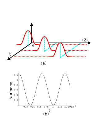
Figure 2: (Color on line) (a) Schematic illustration about the time evolution for the center of the initial Gaussian state of the dark polariton along $z$ direction. (b) the time evolution of the variance in $x$-direction. The variance is in unit of $0.1$.

In plotting Fig. 2 (b), we have taken the reasonable parameters accessible in current exprimentsKarpa : the width of the initial Gaussian $1/\alpha_{x}=1/4$cm, the atomic density $N/V=10^{13}$ per cube centimeter, the quantum number of the ground state $m_{F}^{g}=-2$ with $g_{F}^{g}=1/2$, the quantum number of the mestable state $m_{F}^{s}=0$, and $\gamma_{1}=2\pi\times 2.87$MHz.

V The deflection of dark polaritons in a linear magnetic field

In a recent experiment Karpa , a magnetic field with small transverse gradient is applied to a $\Lambda$-type atomic medium. It was observed that the light beam is deflected after the signal light passing through the EIT gas cell. This observation first demonstrates that quasi-particles - dark-state polaritons have a non-zero magnetic moment. This experimental observation can be interpreted straightforwardly according to the above quantum theory of spatial motion of polaritons in inhomogeneous fields.

For simplicity, we assume the magnetic field

$$B\left(r\right)=B_{0}+B_{1}x\text{.}$$ (44)

has a linear gradient along the $x$-direction. We further allow the input pulse to vary only in one transverse dimension, says, in the $x$-direction, which means that we neglect the $y$-dependence of the input pulse $E$. Then the two dimensional effective Hamiltonian for the dark polaritons reads

$$H_{2}=v_{g}P_{z}+\frac{1}{2m}P_{x}^{2}-\mu b_{0}-\mu\zeta x\text{,}$$ (45)

where the parameters

$$\zeta =2B_{1}\sin^{2}\theta\text{,}$$ (46a)

$$b_{0} =2B_{0}\sin^{2}\theta\text{,}$$ (46b)

$$\mu =\mu_{s}-\mu_{g}$$ (46c)

can be controlled by the mixing angle $$\theta \alpha_{x}=\alpha_{z}=b^{-2} U_{li}\left(t\right)=\exp\left(-iH_{2}t\right) U_{li}\left(t\right) U_{li}\left(t\right)=U_{2}\left(t\right)U_{1}\left(t\right)$$. For an initial dark polariton field with Gaussian spatial distribution as given in Eq. (37), the time evolution of the polariton field reads . By the Wei-Norman algebraic method (see the appendix A) swna , the unitary operator can be factorized as with

$$U_{2}\left(t\right) =e^{-iv_{g}tP_{z}}e^{-i\frac{t}{2m}P_{x}^{2}}e^{it^{2}\frac{\mu\zeta}{2m}P_{x}}\text{,}$$ (47a)

$$U_{1}\left(t\right) =e^{it\mu\zeta x}e^{i\mu b_{0}t-i\frac{t^{3}}{3}\frac{\mu^{2}\zeta^{2}}{2m}}\text{.}$$ (47b)

A straight forward calculation shows that, the initial Gaussian packet evolves into

$$\Psi\left(t\right) =\left(\frac{1/\pi}{b^{2}+i\frac{t}{m}}\right)^{\frac{1}{2}}e^{i\mu t\left(b_{0}-\frac{t^{2}}{3}\frac{\mu\zeta^{2}}{2m}\right)}e^{-\frac{\left(z-v_{g}t\right)^{2}}{2b^{2}}}$$ (48)

$$e^{i\mu\zeta tx}\exp\left[-\frac{\left(x-t^{2}\frac{\mu\zeta}{2m}\right)^{2}\left(b^{2}-i\frac{t}{m}\right)}{2b^{4}+2t^{2}/m^{2}}\right]\text{.}$$

At time $t$, the center of the input pulse moves to $v_{g}t$ along the $z$-direction and $t^{2}\mu\zeta/\left(2m\right)$ along the $x$-direction. When a dark polariton is excitated by the interaction between light and atoms, the dark polariton will achieve a velocity along the $x$-direction as

$$v_{x}=\frac{\mu\zeta L}{mv_{g}}\text{.}$$ (49)

after it pass through the gas cell with length L. Therefore the deflection angle reads

$$\alpha=\frac{v_{x}}{v_{g}}=\frac{L}{v_{g}}\frac{\mu}{k}B_{1}\sin^{2}\theta\text{.}$$ (50)

In real experiment, the dephasing time is nonzero due to the collision between atoms, which leads to the absorption of the energy of the probe beam by the atomic medium.

The above results mean that the deflection angle of the output pulse depends on the mixing angle $\theta$ between the signal field and the collective atomic polarization, the wave number $k$ of the input pulse, and the gradient $B_{1}$ of the inhomogeneous magnetic field. One can find that the magnetic moment of the dark polariton has an effective value

$$\mu_{pol}=\mu\sin^{2}\theta\text{.}$$ (51)

By taking $m_{g}=-2$ and $m_{s}=0$, we find the effective magnetic moment

$$\mu_{pol}=2g_{F}^{(g)}\mu_{B}\sin^{2}\theta\text{,}$$ (52)

which is exactly the theoretical result given in Ref. Karpa .

Next we consider the spatial resolution, which in optics reflects the ability of this optical system to form separate and distinct images of two objects.

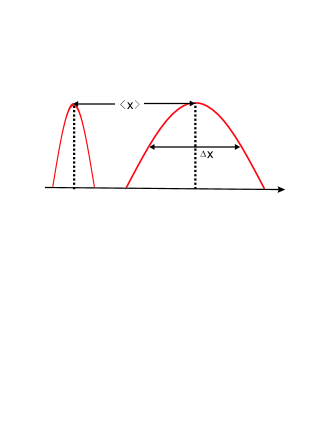
Figure 3: (Color on line)Schematic illustration about the spatial resolution.

The spatial resolution is defined here as the mean signal divided by its standard deviation

$$R=\frac{\left\langle x\right\rangle}{\Delta x}=t^{2}\mu\zeta\sqrt{\frac{b^{2}}{2m^{2}b^{4}+2t^{2}}}\text{,}$$ (53)

where the mean position $\left\langle x\right\rangle$ in the transverse direction and the standard deviation $\Delta x$ are given by

$$\left\langle x\right\rangle =\int_{-\infty}^{+\infty}\Psi^{\ast}\left(t\right)x\Psi\left(t\right)dxdz=t^{2}\frac{\mu\zeta}{2m}\text{,}$$ (54a)

$$\Delta x =\sqrt{\left\langle x^{2}\right\rangle-\left\langle x\right\rangle^{2}}=\sqrt{\frac{m^{2}b^{4}+t^{2}}{2b^{2}m^{2}}}\text{.}$$ (54b)

It can be seen that the spatial resolution increases as the interaction time between light and atoms increases.

Actually, the phenomenon of light deflection in such an inhomogeneous magnetic field can also be described without using the concept of quasiparticles - dark polaritons. Here, we show how to calculate the deflection angle $\alpha$ in Eq. (50) according to the semiclassical theory. We begin the semiclassical approaches by considering the evolution of the system from Eq. (14) and (20). First, the atomic linear response to the signal field has been explicitly reflected in Eq. (20). Under the adiabatic approximation that the evolution of the atomic system is much faster than the temporal change of the radiation field, we can obtain the steady-state solution for the atomic transition $\sigma_{ge}^{(1)}$ by setting all time derivatives to zero in Eq. (20), namely

$$\sigma_{ge}^{(1)} =i\frac{\left[i\left(\mu_{g}-\mu_{s}\right)B+\gamma_{2}\right]g}{d_{1}d_{2}+\left|\Omega\right|^{2}}E$$ (55)

$$\approx\frac{g}{\left|\Omega\right|^{2}}\mu BE.$$

Here, the undepleted control-field approximation is used and $\gamma_{2}\approx 0$ is assumed. This approach based on the atomic linear response results in an effective potential for the motion of signal slow-varying amplitude due to the spatial distribution of the magnetic field. The spatial motion of the slow varying amplitude is described by the following equation:

$$i\frac{\partial}{\partial t}E+ic\frac{\partial}{\partial z}E+\frac{c}{2k}\nabla_{T}^{2}E=-\frac{|g|^{2}N}{\left|\Omega\right|^{2}}\mu BE$$ (56)

$$=-\mu\left(B_{0}+B_{1}x\right)E\tan^{2}\theta$$

which describes a shape-preserving propagation in $z$ direction with velocity $c$.

For an initial Gaussian wave packet of $E$ in $x-z$ plane, after passing through the gas cell, the wave center shifts from $\left(x,z\right)=\left(0,0\right)$ to the well-defined position

$$\left(x,z\right)=\left(\frac{\mu B_{1}}{2kc}L^{2}\tan^{2}\theta,L\right)\text{.}$$ (57)

And it can be obviously found that Eq. (50) is the deflection angle in this approach.

VI Deflection of light in inhomogeneous coupling field

In this section, we turn our discussion to the deflection of slow light in the atomic medium driven by a optical field with an inhomogeneous profile, while the magnetic field is uniform. This phenomenon was experimentally observed in Ref. Scul07 where the cell filled with EIT-based atomic gas is referred as an ultra-dispersive optical prism with an angular dispersion. We note that the probe light is relatively strong in comparison with the control light in this experiment, thus the susceptibility obtained from the linear response theory can not work well to explain the experiment phenomenon. In this paper, we do not plan to explain the experiment data in Ref. Scul07 in the strong coupling limit. Our main purpose is to predict a new quantum coherent phenomenon for the light deflection by the atomic media when the experiment is carried out for the weak probe field.

We assume the strong driving field has a Gaussian profile

$$\Omega=\Omega_{0}\exp\left[-\frac{x^{2}}{2\sigma^{2}}\right]$$ (58)

in the transverse direction. Here, we confine the problem to two dimensional space, the $x$-$z$ plane. Then the transverse Laplacian operator reduces into a one dimensional operator $\nabla_{T}^{2}=\partial^{2}/\partial x^{2}$.

By invoking the steady-state conditions, it is found that the polarization field $\sigma_{ge}^{(1)},$ which serves as a source for the electric fields in Eq. (14), is proportional to the slow varying amplitude $E$ given in Eq. (55). Under a strong, undepleted driving field approximation, the coupling between atoms and light induces a spatial dependent potential into the propagation equation. The spatial shape of this potential induced by $\sigma_{ge}^{(1)}$ is completely determined by the profile of the Rabi frequency $\Omega$, which can be seen in the first line of Eq. (56 ). Thus, when the signal pulse parallel to the control beam travels across the atomic cell, it will be scattered by the effective potential. However, as the width of probe beam is less than that of the control beam, the trajectory of the probe light may bend when it is adjusted to the left side or to the right side of the control beam profile; hence the probe and control beams are no longer parallel after they go through the gas cell.

In order to investigate this phenomenon, we assume the probe beam is in a Gaussian state

$$E\left(0,x,z\right)=\frac{1}{\sqrt{\pi b^{2}}}\exp\left[-\frac{\left(x-a\right)^{2}}{2b^{2}}-\frac{z^{2}}{2b^{2}}\right]$$ (59)

before it enters the gas cell, where $b$($<\sigma$) is the width of the probe field and $a$ is the initial location of the wave packet center of the probe field along $x$-direction. The sign of $a$ indicates the incident position comparatively to the left or right hand side of the control beam’s center $x_{0}=0$, and the magnitude $\left|a\right|$ denotes the distance from the control beam’s center. In order to investigate the evolution of this initial state, we expand $\left|\Omega\right|^{-2}$ at the position $a$ and retain the linear term proportional to $x-a$.

With the above considerations, the paraxial equation in Eq. (56) becomes

$$i\dot{E}+ic\partial_{z}E+\frac{c}{2k}\partial_{x}^{2}E=\left(\eta_{0}+\eta_{1}x\right)E$$ (60)

where

$$\eta_{0} =-\Omega_{0}^{-2}\left(1-\frac{2a^{2}}{\sigma^{2}}\right)|g|^{2}N\Delta\exp\left(\frac{a^{2}}{\sigma^{2}}\right)\text{,}$$ (61a)

$$\eta_{1} =-2a\Delta\frac{|g|^{2}N}{\sigma^{2}}\Omega_{0}^{-2}\exp\left(\frac{a^{2}}{\sigma^{2}}\right)\text{.}$$ (61b)

and $$\Delta=\left(\mu_{s}-\mu_{g}\right)B \left(x,z\right)=\left(a,0\right) t=0$$. By making use of the Wei-Norman algebraic method swna , it is shown that, after passing through the Rb gas cell, the center position of the probe field at time is shifted to

$$x =a+L^{2}\Omega_{0}^{-2}\Delta ae^{\frac{a^{2}}{\sigma^{2}}}\frac{|g|^{2}N}{\sigma^{2}kc}\text{,}$$ (62a)

$$z =L\text{.}$$ (62b)

If we track the motion of the center of the probe beam, a mirage effect occurs. The sign of $\Delta$ and the incident position $a$ of the signal light determine whether the trajectory of probe beam bend. When the magnetic field is absent $\Delta=0$ or the center of the probe field is collinear to that of the control field $a=x_{0}=0$, the trajectory of the signal light is a straight line. We assign the positive sign for $a$ as the probe beam is shifted to the right with respect to the center of the control light, and denote $a<0$ as the signal beam is shifted to the left. When the probe beam is shifted to the right, in the case of $\Delta<0$, the signal light feels a “repulsion potential” due to the coefficient $\eta_{1}>0$, thus the trajectory bends to the left; at the condition $\Delta>0$, the signal light undergoes an “attractive potential” in the atomic medium due to $\eta_{1}<0$, thus the trajectory bends to the right. When $a<0$, it can be found from Eq. (61) that due to the coefficient of the linear potential larger than zero, i.e. $\Delta>0$, the probe beam experiences a “repulsion potential” within the EIT medium, and its center is shifted to the left. As $\eta_{1}$ is smaller than zero, i.e. $\Delta<0$, the probe beam suffers an “attractive potential” during its passing through the EIT medium, hence its center is shifted to the right. The corresponding schematic diagram is given in Fig.4, where yellow solid line is the spatial distribution of the

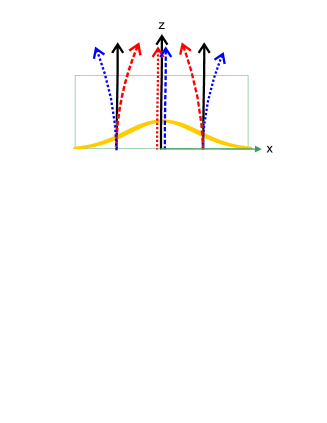
Figure 4: (Color on line)Schematic illustration about the ray deflection of the probe light in the presence of inhomogenous coupling light. The yellow line is the spatial distribution of the control light.

control light, the red dash lines give the deflection at $\Delta<0$, the blue dotted lines describe the light trajectory at $\Delta>0$ and the black solid lines depict the light ray at $\Delta=0$. The same results about the deflection of light ray have been discovered by us using the semiclassical theory ZDL .

From the point of particle nature, the force acting on the particle is completely determined by the value and sign of $\eta_{1}$. Thus for a particle passing through the point $a\neq 0$, when $\Delta=0$, the particle does not feel any force, so it travels across straightly, so does the particle at point $a=0$. For a particle traversing through the position $a\left(>0\right)$, when $\Delta<0$, this particle is subject to a negative force, which moves the particle to the left with respect to it original place; however, when $\Delta>0$, it experiences a positive force, which makes the particle move to the right. Also for a particle going through the place at $a(<0)$, when $\Delta<0$, the particle moves to the right because of the action of a positive force; when $\Delta>0$, it goes to the left due to the action of a negative force.

We have to point out that the magnetic field is not necessary for the occurrence of the above-described phenomenon. For the model containing a $\Lambda$-type atomic ensemble interacting with one control beam and one probe beam, similar phenomenon can also be found as long as the two photon detuning

$$\Delta=\Delta_{p}-\Delta_{c}$$ (63)

varies, where $\Delta_{p}=\omega_{eg}-\nu$ is the detuning between the atomic transition from $\left|e\right\rangle$ to $\left|g\right\rangle$ and the probe beam, $\Delta_{c}=\omega_{es}-\nu_{c}$ is the detuning between the atomic transition from $\left|e\right\rangle$ to $\left|s\right\rangle$ and the control beam. In order to clarify the dependence of light deflection on two photon detuning $\Delta$, we begin our description with the Hamiltonian in the interaction picture. In the rotating frame with respect to

$$H_{0}=\omega_{e}\sigma_{ee}+\left(\omega_{s}+\Delta_{c}\right)\sigma_{ss}+\left(\omega_{g}+\Delta_{p}\right)\sigma_{gg}\text{,}$$

the interaction Hamiltonian reads

$$H_{I}^{\prime}=-\frac{N}{V}\int d^{3}r[\Delta_{p}\sigma_{gg}+\Delta_{c}\sigma_{ss}+\left(g\sigma_{eg}E+\Omega\sigma_{es}+h.c.\right)]\text{,}$$

in the absence of magnetic field. The first order atomic transition operators have the similar form as Eq.(20) by replacing $\mu_{s}B$, $\mu_{g}B$ and $\mu_{e}B$ by $\Delta_{c}$, $\Delta_{p}$ and zero respectively. Then the atomic transition operator $\sigma_{ge}^{(1)}=g\Delta E/\left|\Omega\right|^{2}$, which induces a potential dependent on the two photon detuning $\Delta$.

In a real experiment, the dephasing rate of the forbidden $\left|e\right\rangle$-$\left|s\right\rangle$ transition is nonzero due to atomic collisions etc. Therefore an additional anti-Hermitian decay term will be introduced phenomenologically into the effective Hamiltonian

$$H_{eff}=cp_{z}+\frac{c}{2k}p_{x}^{2}+\eta_{0}^{\prime}+\eta_{1}^{\prime}\left(x-a\right)\text{,}$$ (64)

where $\eta_{j}^{\prime}=-a_{j}-ib_{j}$, $j=0,1$ are complex. Then it can be found that, after light passing through the Rb gas cell, the dephasing rate introduces two additional terms to Eq. (62a)

$$x=a+\frac{a_{1}c}{2k}T^{2}-b^{2}b_{1}T-\frac{b_{1}c^{2}}{b^{2}k^{2}}T^{3}$$ (65)

where $T=L/c$ is the time for the light travelling through the medium, and

$$a_{1} = \frac{2a}{\sigma^{2}}\frac{N\left|g\right|^{2}}{\Omega_{0}^{2}}\exp\left(\frac{a^{2}}{\sigma^{2}}\right)\Delta\text{,}$$

$$b_{1} = \frac{2a}{\sigma^{2}}\frac{N\left|g\right|^{2}}{\Omega_{0}^{2}}\exp\left(\frac{a^{2}}{\sigma^{2}}\right)\gamma_{2}\text{.}$$

For an atomic medium with length $L=7.5cm$ and density $N/V=10^{12}cm^{-3}$, the dephasing rate $\gamma_{2}\approx 10^{-4}\gamma_{1}$. When a control beam with width $\sigma=L/4$ and frequency $\nu_{c}=5\times 10^{14}Hz$ is coupled to the atomic ensemble with $\Omega_{0}=5\gamma_{1}$, for the probe beam with width $0.07mm$ incident at position $a=\sigma/2$, two additional terms $b^{2}b_{1}T\approx 10^{-3}$ and $b_{1}c^{2}T^{3}/(b^{2}k^{2})\approx 10^{-5}$ caused by dephasing are much smaller than that of the term $a_{1}cT^{2}/(2k)\approx 5\times 10^{-2}$ induced by the frequency detuning $\Delta$, which means Eq. (62a) dominates the distance in the transverse direction.

Next we investigate how the trajectory of the probe beam behaves when an effective potential include the quadratic term of $x$ and $y$ in the transverse direction. This induced potential is obtained when we expand

$$\left|\Omega\right|^{-2}=\Omega_{0}^{-2}\exp\left[\frac{x^{2}}{\sigma_{x}^{2}}+\frac{y^{2}}{\sigma_{y}^{2}}\right]$$ (66)

around the center $a_{x}$ and $a_{y}$ of the incident beam with the profile shape

$$E\left(0\right)=\frac{1}{\sqrt{\pi b^{2}}}\exp\left[\frac{z^{2}+\left(x-a_{x}\right)^{2}+\left(y-a_{y}\right)^{2}}{-2b^{2}}\right]\text{.}$$ (67)

By retaining the quadratic term of $x-a_{x}$ and $y-a_{y}$. The paraxial motion equation becomes

$$i\partial_{t}E+ic\partial_{z}E+\frac{c}{2k}\left(\partial_{x}^{2}+\partial_{y}^{2}\right)E=\left[V\left(x\right)+V\left(y\right)\right]E$$ (68)

where

$$V\left(\chi\right)=\left[\zeta_{\chi 0}+\zeta_{\chi 1}\left(\chi-a_{\chi}\right)+\zeta_{\chi 2}\left(\chi-a_{\chi}\right)^{2}\right]E\text{.}$$

The coefficients for $\chi=\left\{x,y\right\}$ are

$$\zeta_{\chi 0} =-\Omega_{0}^{-2}\exp\left[\frac{a_{\chi}^{2}}{\sigma_{\chi}^{2}}\right]\text{,}$$ (69a)

$$\zeta_{\chi 1} =-\frac{2|g|^{2}N}{\sigma_{\chi}^{2}}a_{\chi}\Delta\Omega_{0}^{-2}\exp\left[\frac{a_{\chi}^{2}}{\sigma_{\chi}^{2}}\right]\text{,}$$ (69b)

$$\zeta_{\chi 2} =-\frac{\sigma_{\chi}^{2}+2a_{\chi}^{2}}{2\sigma_{\chi}^{4}}\Omega_{0}^{-2}|g|^{2}N\Delta\exp\left[\frac{a_{\chi}^{2}}{\sigma_{\chi}^{2}}\right]\text{.}$$ (69c)

After a period of time, the Gaussian state will evolve into

$$E\left(t\right)=U\left(t\right)E\left(0\right)$$ (70)

where the evolution operator

$$U\left(t\right)=\exp\left[-i\left(cP_{z}+\frac{P_{x}^{2}+P_{y}^{2}}{2m^{\prime}}+V\left(x\right)+V\left(y\right)\right)t\right]$$ (71)

Here, we assume that the detuning $\Delta$ is always negative. The Schrö dinger-type equation (68) governs the evolution of the wave-function of the signal light in the atomic medium. And the trajectory of light ray is described by the mean value of the coordinate operator

$$\chi_{c}=\left\langle\chi\right\rangle=\int E^{\ast}(t)\chi E(t)d\chi\text{,}$$ (72)

with $\chi\in\left\{x,y,z\right\}$. An explicit calculation gives (see Appendix B)

$$x_{c} =a_{x}-\zeta_{x1}\frac{1-\cos\left(\omega_{ox}t\right)}{m^{\prime}\omega_{ox}^{2}}\text{,}$$ (73a)

$$y_{c} =a_{y}-\zeta_{y1}\frac{1-\cos\left(\omega_{oy}t\right)}{m^{\prime}\omega_{oy}^{2}}\text{,}$$ (73b)

$$z_{c} =ct$$ (73c)

with the angular frequency

$$\omega_{ox}=\sqrt{2\zeta_{x2}/m^{\prime}}\text{, }\omega_{oy}=\sqrt{2\zeta_{y2}/m^{\prime}}\text{.}$$ (74)

As the light travels across the atomic medium, the light ray - the center of the wave packet oscillates around the initial center in the transverse direction

$$x_{c} =a_{x}+\frac{\zeta_{x1}}{m^{\prime}\omega_{ox}^{2}}\left(\cos\frac{\omega_{ox}z_{c}}{c}-1\right)\text{,}$$ (75a)

$$y_{c} =a_{y}+\frac{\zeta_{y1}}{m^{\prime}\omega_{oy}^{2}}\left(\cos\frac{\omega_{oy}z_{c}}{c}-1\right)\text{.}$$ (75b)

The anisotropic motion and potential in Eq. (68) result in that, light travels in a straight line in the $$z$$-direction since it acts as an

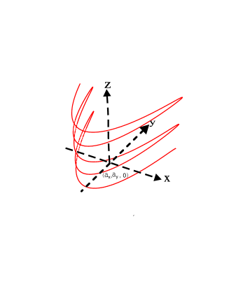
Figure 5: (Color on line)Schematic illustration about the ray trajectory of the probe light in three dimension space.

ultra-relativistic particle with velocity $c$, however the light oscillates in the $x$-$y$ plane because it behaves as a non-relativistic particle with effective transverse mass $m^{\prime}=k/c$. If $\zeta_{x2}=\zeta_{y2}$, the light ray is a line with finite length in the transverse direction. In Fig. 5, we schematically illustrate the wave packet center of the probe light in three-dimension space when $\zeta_{x2}\neq\zeta_{y2}$.

VII Summary

In conclusion, we have developed a quantum approach for the spatial behavior of propagating light when it passes through an EIT system with spatial-dependent external fields. By studying the dynamics of the atomic ensemble and the light pulse, the effective Schrödinger equation is derived to depict the space-time evolution of quasi-particles where the effective potential is induced through the steady atomic response in the external spatial-dependent fields. For a magnetic field with a spatial distribution in the transverse direction, by considering the evolution of the Gaussian state, we showed that: 1) in a harmonic magnetic field, the light trajectory is a straight line; 2) in a linear magnetic field, the light ray bends to the direction where the magnetic gradient increases. And the deflection angle depends on four external parameters: the mixing angle between the signal field and the collective atomic polarization, the wave number of the signal pulse, the length of the EIT gas cell, and the small magnetic field gradient. In an inhomogeneous optical control field, we predict some novel results accessible on the light ray behavior. In the linear response limit, it is found that the deflection of the light ray can be controlled by two controllable external parameters: the center position of the probe beam with respect to the control light, and the two photon detuning. In the quadric expansion of coupling amplitude, the light trajectory generally oscillates in the atomic medium.

Finally we note that our study is based on a quantum theoretical approach. In our previous paper ZDL , the Fermat principle is applied to study the light trajectory in this atomic medium, and similar results are obtained, but that approach is a semi-classical theory , which can be understood in terms of the eikonal equation with the optical WKB approximation of our approach. Though this semi-classical approach can explain the most recent experiment Karpa about the light deflection by an EIT-based rubidium gas, it can not be further developed for the investigation of photon state quantum storage since the signal light was assumed as a classical field. The quantum approach assumes the probe light is quantized, thus this approach can be used to investigate the possibility for realizing a protocol for quantum sate storage with spatially-distinguishable channels based on the EIT-enhanced light deflection.

This work is supported by the NSFC with Grants No. 90203018, No. 10474104, No. 60433050 and No. 10704023, NFRPC with Grant No. 2001CB309310 and 2005CB724508. One (LZ) of the authors also acknowledges the support of K. C. Wong Education Foundation, Hong Kong. We acknowledge the useful discussions with P. Zhang, T. Shi, and H. Ian.

Appendix A Factorization of unitary operator $U_{li}$

Since the unitary operator $U_{li}$ is exponential, factorizing it means to express the exponential of a sum of operators in terms of a product of the exponentials of operators. The unitary operator $U_{li}$ is an element of the group  generated by the momentum operators $P_{z}$, $P_{x}$ and the coordinate $x$. Since $P_{z}$ commutes with $P_{x}$ and $x$, the unitary operator can first be factorized as

$$U_{li}=e^{-iv_{g}tP_{z}}U_{li}^{\prime},$$ (76)

where

$$U_{li}^{\prime}=\exp\left[-i\left(\frac{1}{2m}P_{x}^{2}-\mu b_{0}-\mu\zeta x\right)t\right]$$ (77)

only contains operator $P_{x}$ and $x$, which generate the Lie algebra with the basis $\{x,P_{x},P_{x}^{2},\mathbf{1}\}.$ Thus, operator $U_{li}^{\prime}$ can be factorized as the form

$$U_{li}^{\prime}=e^{g_{1}P_{x}^{2}}e^{g_{2}P_{x}}e^{g_{3}x}e^{g_{4}},$$ (78)

and $g_{i}=g_{i}(t)$ are unknown functions of time $t$ to be determined.

Mathematically, the above factorization Ansatz is based on the Wei-Norman algebraic theorem swna : if the Hamiltonian of a quantum system

$$H=\sum_{j=1}^{K}C_{j}(t)X_{j}$$ (79)

is a linear combination of the operators $X_{j}$ that can generate a $N$-dimensional Lie algebra with the basis:

$$\{X_{1},X_{2},...,X_{k},X_{k-1},....X_{N}\},$$ (80)

then the evolution operator governed by $H$ can be factorized as a product of the single parameter subgroups, that is ,

$$U=\prod\limits_{j-1}^{N}e^{\xi_{j}(t)X_{j}},$$ (81)

where the coefficients $\xi_{j}(t)$ can be determined the “external field parameters” $C_{j}(t)$ through a system of non-linear equations.

Now, we differentiate (78) with respect to $t$ and the multiply the resulting expression on the right hand side by the inverse of (78), obtaining

$$\frac{1}{2m}P_{x}^{2}-\mu\zeta x-\mu b_{0}=$$ (82a)

$$i\frac{\partial g_{1}}{\partial t}P_{x}^{2}+iP_{x}\left(\frac{\partial g_{2}}{\partial t}-2ig_{1}\frac{\partial g_{3}}{\partial t}\right)$$

$$+ix\frac{\partial g_{3}}{\partial t}+i\left(\frac{\partial g_{4}}{\partial t}-ig_{2}\frac{\partial g_{3}}{\partial t}\right).$$

This leads to a systems of coupled differential equations

$$i\frac{\partial g_{1}}{\partial t}=\frac{1}{2m}\text{, }$$ (83a)

$$i\frac{\partial g_{3}}{\partial t}=\mu\zeta\text{, }$$ (83b)

$$i\left(\frac{\partial g_{2}}{\partial t}-2g_{1}i\frac{\partial g_{3}}{\partial t}\right)=0,$$ (83c)

$$i\left(\frac{\partial g_{4}}{\partial t}-i\frac{\partial g_{3}}{\partial t}g_{2}\right)=\mu b_{0}.$$ (83d)

The solution to these equations reads

$$g_{1} =-i\frac{t}{2m}\text{, }$$ (84a)

$$g_{3} =it\mu\zeta,$$ (84b)

$$g_{2} =i\frac{\mu\zeta}{2m}t^{2}\text{,}$$ (84c)

$$g_{4} =i\mu\left(b_{0}t-\frac{t^{3}}{3}\frac{\mu\zeta^{2}}{2m}\right).$$ (84d)

Therefore the unitary operator $$U_{li}$$ is factorized into the form given in Eq. (47).

Appendix B Calculation of light trajectory in quadratic potential

In the presence of the quadratic term of coordinates, the evolution operator $U\left(t\right)$ in Eq. (68) is generated by the effective Hamiltonian $H_{3}=H_{z}+H_{y}+H_{x}$:

$$H_{z} =cP_{z}\text{,}$$ (85)

$$H_{y} =\frac{P_{y}^{2}}{2m^{\prime}}+V\left(y\right)\text{,}$$ (86)

$$H_{x} =\frac{P_{x}^{2}}{2m^{\prime}}+V\left(x\right)\text{.}$$ (87)

The evolution operator can be factorized as

$$U\left(t\right)=U_{z}\left(t\right)U_{y}\left(t\right)U_{x}\left(t\right)$$ (88)

with

$$U_{z} =U_{z}\left(t\right)=e^{-iH_{z}t}\text{,}$$ (89)

$$U_{y} =U_{y}\left(t\right)=e^{-iH_{y}t}\text{,}$$ (90)

$$U_{x} =U_{x}\left(t\right)=e^{-iH_{x}t}\text{.}$$ (91)

The expectation value of the coordinator along $x$-direction is calculated as

$$\left\langle x\right\rangle =\int E^{\ast}\left(0\right)U^{{\dagger}}\left(t\right)xU\left(t\right)E\left(0\right)dx$$ (92)

$$=\int E^{\ast}\left(0\right)U_{x}^{{\dagger}}xU_{x}E\left(0\right)dx$$

$$=a_{x}+\int E^{\ast}\left(0\right)U_{x}^{{\dagger}}\left(x-a_{x}\right)U_{x}E\left(0\right)dx$$

where commutation relation $\left[x,P_{\chi}\right]=i\delta_{\chi x}$ is used to obtain the second identity in Eq. (92).

Actually, the effective Hamiltonian $H_{x}$ describes a harmonic oscillator with its origin displaced from $a_{x}$ to other place. Thus, we rewrite the coordinate and momentum operators in terms of the creation and annihilation operator $\left\{d^{{\dagger}},d\right\}$:

$$\eta =\frac{1}{\sqrt{2m^{\prime}\omega_{ox}}}\left(d^{{\dagger}}+d\right),$$ (93)

$$P_{\eta} =i\sqrt{\frac{m^{\prime}\omega_{ox}}{2}}\left(d^{{\dagger}}-d\right)$$ (94)

with the inverse relation

$$d =\sqrt{\frac{m^{\prime}\omega_{ox}}{2}}\eta+i\sqrt{\frac{1}{2m^{\prime}\omega_{ox}}}P_{\eta},$$ (95)

$$d^{{\dagger}} =\sqrt{\frac{m^{\prime}\omega_{ox}}{2}}\eta-i\sqrt{\frac{1}{2m^{\prime}\omega_{ox}}}P_{\eta},$$ (96)

where $\eta=x-a_{x}$ and $\omega_{ox}$ is given in Eq. (74). The effective Hamiltonian $H_{x}$ can be diagonalized as

$$H_{x}=\omega_{ox}\left(d^{\dagger}d+\frac{1}{2}\right)$$ (97)

by a displacement operator

$$D\left(\beta\right)=\exp\left(\beta d^{\dagger}-\beta^{\ast}d\right)$$ (98)

with

$$\beta=\beta^{\ast}=-\frac{\zeta_{x1}}{\omega_{ox}\sqrt{2m^{\prime}\omega_{ox}}}\text{.}$$ (99)

Then the evolution operator is factorized as the product of three operators

$$U_{x}=D\left(\beta\right)e^{-i\omega_{ox}\left(d^{\dagger}d+\frac{1}{2}\right)t}D^{-1}\left(\beta\right)\text{.}$$ (100)

In terms of the creation and annihilation operators, the center of the light wave packet

$$\left\langle x\right\rangle =a_{x}+\frac{\cos\left(\omega_{ox}t\right)}{\sqrt{2m^{\prime}\omega_{ox}}}\int E^{\ast}\left(0\right)\left(d^{\dagger}+d\right)E\left(0\right)dx$$

$$+i\frac{\sin\left(\omega_{ox}t\right)}{\sqrt{2m^{\prime}\omega_{ox}}}\int E^{\ast}\left(0\right)\left(d^{\dagger}-d\right)E\left(0\right)dx$$

$$-2\frac{\beta\cos\left(\omega_{ox}t\right)}{\sqrt{2m^{\prime}\omega_{ox}}}+\frac{2\beta}{\sqrt{2m^{\prime}\omega_{ox}}}$$ (101)

Back to the coordinate and momentum operators, the center of the wave packet in $x$-direction is obtained as Eq. (73a). In a similar way, Eq. (73b) can be achieved.

References

- (1) R.D. Mattuck, A Guide to Feynman Diagrams in the Many-body Problem, Dover Books on Physics and Chemistry:NY, 1967.
- (2) C. Liu, Z. Dutton, C. H. Behroozi, and L. V. Hau, Nature 409, 490 (2001);
- (3) L. V. Hau, S. E. Harris, Z. Dutton, and C. H. Behroozi, Nature 397, 594 (1999).
- (4) S. E. Harris, Phys. Today 50, No. 7, 36 (1997).
- (5) S. E. Harris and L. V. Hau, Phys. Rev. Lett. 82, 4611 (1999).
- (6) M. Fleischhauer and M. D. Lukin, Phys. Rev. Lett. 84, 5094 (2000).
- (7) M. Fleischhauer and M. D. Lukin Phys. Rev. A 65, 022314 (2002).
- (8) M. Fleischhauer, A. Imamoglu, J. P. Marangos, Rev. Mod. Phys. 77, 633 (2005).
- (9) M. D. Lukin, Rev. Mod. Phys. 75, 457 (2003).
- (10) C. P. Sun, Y. Li and X. F. Liu, Phys. Rev. Lett. 91, 147903 (2003).
- (11) L. Karpa, M.Weitz, Nature Physics 2, 332 (2006).
- (12) V. A. Sautenkov, H. Li, Y. V. Rostovtsev, M. O. Scully, e-print arXiv:quant-ph/0701229.
- (13) D. L. Zhou, L. Zhou, R. Q. Wang, S. Yi, C. P. Sun, Phys. Rev. A 76, 055801 (2007).
- (14) M. O. Scully, M. Zubairy, Quantum optics, (Cambridge University Press, 1997).
- (15) J. Wei and E. Norman, J. Math. Phys. 4A, 575 (1963)