Nonperturbative Scaling Theory of Free Magnetic Moment Phases in Disordered Metals

Abstract

The crossover between a free magnetic moment phase and a Kondo phase in low dimensional disordered metals with dilute magnetic impurities is studied. We perform a finite size scaling analysis of the distribution of the Kondo temperature as obtained from a numerical renormalization group calculation of the local magnetic susceptibility and from the solution of the self-consistent Nagaoka-Suhl equation. We find a sizable fraction of free (unscreened) magnetic moments when the exchange coupling falls below a disorder-dependent critical value $J_{\rm c}$. Our numerical results show that between the free moment phase due to Anderson localization and the Kondo screened phase there is a phase where free moments occur due to the appearance of random local pseudogaps at the Fermi energy whose width and power scale with the elastic scattering rate $1/\tau$.

The Kondo problem is of central importance for understanding low-temperature anomalies in low-dimensional disordered metals dcmreview ; miranda ; bhatt ; zu96 ; jetpletters ; micklitz05 ; meraikh ; lw04 ; kbu042 ; kbu03 ; grempel ; micklitz06 , such as the saturation of the dephasing rate bergmann and the non-Fermi-liquid behavior of certain magnetic alloys bernal ; dcmreview . For a clean metal, the screening of a spin-$1/2$ magnetic impurity is governed by a single energy scale, the Kondo temperature $T_{K}$. Thermodynamic observables and transport properties obey universal functions which scale with $T_{K}$. Thus, in a metal where nonmagnetic disorder is also present, two fundamental questions naturally arise: (i) Is the Kondo temperature modified by nonmagnetic disorder? (ii) Is the one-parameter scaling behavior still valid? It is well known miranda ; meraikh ; dcmreview ; jetpletters ; grempel that magnetic moments remain unscreened when conduction electrons are localized due to disorder. However, in weakly disordered two-dimensional electron systems, the localization length is macroscopically large, and so is the number $N_{\rm c}$ of eigenstates with a finite amplitude at the position of the magnetic impurity. In this case, one does not expect to find unscreened magnetic moments for experimentally relevant values of the exchange coupling $J$.

Another situation where magnetic moments remain free in metals at low temperatures occurs when the density of states has a global pseudogap at the Fermi energy $E_{\rm F}$, namely, $\nu(E)\sim(E-E_{\rm F})^{\alpha}$, where $\alpha>0$ gapless . In clean metals, the pseudogap quenches the Kondo screening when $J$ falls below a critical value $J_{\rm c}(\alpha)$. So far, only a few values of $\alpha$ have been realized experimentally: $\alpha=1$ in graphene and in $d$-wave superconductors and $\alpha=2$ in $p$-wave superconductors. In this Letter we examine the quantum phase diagram of magnetic moments diluted in two-dimensional disordered metals using a modified version of the numerical renormalization group (NRG) method. We find a free moment phase which we attribute to the random occurrence of local pseudogaps. The existence of free moments is confirmed directly with NRG by the Curie-like behavior of the the local magnetic susceptibility at low temperatures. Finite-size scaling is performed to demonstrate the robustness of our finding. Furthermore, the distribution of Kondo temperatures obtained numerically from NRG is found to agree well with earlier results based on the solution of the Nagaoka-Suhl equation jetpletters ; grempel .

We consider the Kondo Hamiltonian of a magnetic impurity diluted in a disordered metal,

$$H_{\rm sd} = \sum_{n\sigma}E_{n}c_{n\sigma}^{\dagger}c_{n\sigma}+\frac{1}{2}\sum_{n,n^{\prime}}J_{nn^{\prime}}\left[S^{+}c_{n\downarrow}^{\dagger}c_{n^{\prime}\uparrow}\right.$$ (1)

$$\ \left.+S^{-}c_{n\uparrow}^{\dagger}c_{n^{\prime}\downarrow}+S_{z}\left(c_{n\uparrow}^{\dagger}c_{n^{\prime}\uparrow}-c_{n\downarrow}^{\dagger}c_{n^{\prime}\downarrow}\right)\right].$$

Here, $E_{n}$ are the eigenenergies of the noninteracting conduction electrons in the disordered metal, which we describe by the Anderson tight binding model,

$$H_{\rm V}=-t\sum_{\langle ij\rangle~{}\sigma}\left(c_{i\sigma}^{\dagger}c_{j\sigma}+{\rm H.c.}\right)+\sum_{i=1~{}\sigma}^{N}V_{i}\,c_{i\sigma}^{\dagger}c_{i\sigma},$$ (2)

with band width $D$, nearest-neighbor hopping amplitude $t$, and random site potentials $V_{i}$, drawn from a flat box distribution of width $W$ centered at zero. We consider square lattices of length $L$ with $N=L^{2}$ sites and periodic boundary conditions. The exchange coupling matrix elements are then given by $J_{nn^{\prime}}=J\,\psi_{n}^{*}({\bf r})\psi_{n^{\prime}}({\bf r})$, with $\psi_{n}({\bf r})$ being the amplitude of the single-electron eigenfunction at the position ${\bf r}$ of the magnetic impurity. Energies are given in units of $t$.

Finite-Size Scaling. First, we obtain all eigenenergies and eigenfunctions of $H_{V}$ by using state-of-the-art numerical diagonalization techniques for a large set of realizations of the potential $V$ zharekeshev . Within one-loop approximation, the Kondo temperature is then obtained from the solution of the Nagaoka-Suhl equation (NSE) suhl ,

$$1=\frac{J}{2N}\sum_{n=1}^{N}\frac{L^{2}|\psi_{n}({\bf r})|^{2}}{E_{n}-E_{\rm F}}\tanh\left(\frac{E_{n}-E_{\rm F}}{2T_{K}}\right).$$ (3)

We assume that $E_{\rm F}$ is between energy levels, with even number of electrons in the ground state of the system. For odd number of electrons, the single electron at the Fermi energy forms a singlet with the magnetic impurity with binding energy $J$. Solving Eq. (3) numerically, one finds strong deviations from the Gaussian behavior even for weak disorder jetpletters . Figure 1 shows for $W=3$ that a double-peak structure persists as the lattice size is increased from 900 to 4,900 sites. This structure evolves into a power-law divergence in the strong-disorder limit jetpletters ; grempel . In order to verify that these features are not an artifact of the one-loop approximation, we performed a comparative analysis of the Kondo temperatures obtained with the nonperturbative NRG method for different system sizes and disorder strengths.

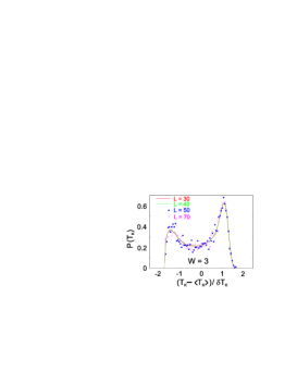
Figure 1: (Color online) The distribution function of Kondo temperatures obtained from the NSE [Eq. (3)] for electrons in tight-binding square lattices with disorder $W=3$. Ensembles of $100$ samples of size $L=30$, 5 samples for $40$, and one sample for $L=50,70$ were used. The exchange coupling was fixed to $J/D=0.35$.

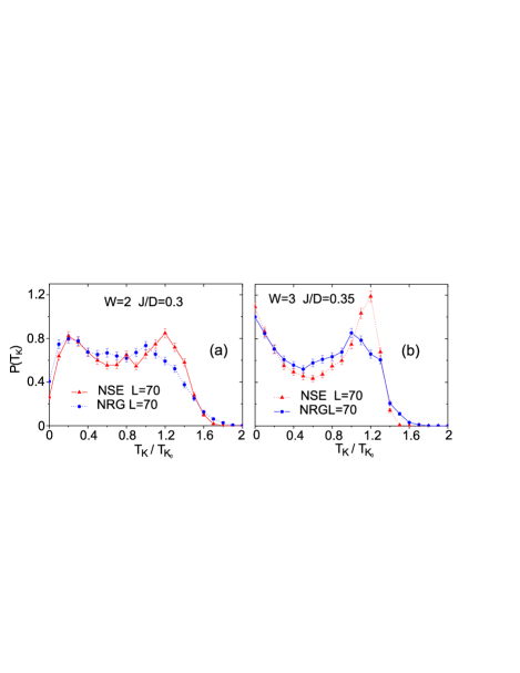
Figure 2: (Color online) The distribution of Kondo temperatures obtained with NRG for lattices of size $L=70$. (a) $W=2$, $J/D=0.3$. (b) $W=3$, $J/D=0.35$ for one realization of the disorder potential. For comparison we plot the distribution obtained from NSE. Higher loop corrections are accounted for by rescaling $T_{K}$ with $0.7\sqrt{J/D}$. The error bars denote the statistical error.

Figure 3: The local spin susceptibility as function of temperature calculated with NRG for exchange coupling $J/D=0.35$, disorder amplitude $W=2$, and lattice size $L=70$. (a) At a site where $T_{K}$ is maximal. Dots: Results obtained with the continuous-time Quantum Monte Carlo method (CT-QMC) rubtsov ; gorelov . (b) At a site where the magnetic impurity remains free. The arrows indicate the Kondo temperature of the clean system for the particular value of $J/D$. Insets: The absolute value square of the eigenfunction amplitudes at those sites as function of energy $E$, where $E=0$ denotes the Fermi energy. The mark indicates the mean level spacing $\Delta$. Energies and temperatures are given in units of $t$.

NRG for Disordered Systems. In order to apply the NRG method to disordered systems, we use as a basis set the eigenfunctions and eigenenergies of the the tight-binding model, Eq. (2), as obtained by the numerical exact diagonalization. We perform the Wilson logarithmic discretization of the conduction band and replace the interval of eigenenergies between $(D/2)\Lambda^{-n+1}$ and $(D/2)\Lambda^{-n},\ n=0,1,2,...$, by one energy level equal to the average of eigenenergies in this interval. The NRG discretization parameter is set to the smallest tractable value, $\Lambda=1.5$. Next, with the help of the well-known tridiagonalization procedure, we numerically map this model onto a discrete Wilson chain. Then, we use an iterative diagonalization procedure, keeping 1,500 states after each iteration wilson . We calculate the local magnetic susceptibility $\chi_{\rm loc}(T)$, which is proportional to the local correlation function of the impurity spin. The susceptibility is found to have a smooth temperature dependence (see Fig. 3) which can be used to define $T_{K}$ through the following criterion: $T\chi_{\rm loc}(T)$ crosses over from the free spin value $1/4$ to a decay linear in $T$ as the temperature is lowered below the Kondo temperature $T_{K}$. For a clean flat band system, $\chi_{\rm loc}(T)$ coincides with the impurity susceptibility $\chi_{\rm imp}$, which is obtained as the difference between the susceptibility of the electronic system with and without the impurity clogston ; hewson . Wilson defined the Kondo temperature as the crossover temperature where $T_{K}\chi_{\rm imp}(T_{K})=0.07$ wilson ; krishna . For disordered systems, we find that $T\chi_{\rm imp}(T)$ can strongly deviate from the universal scaling curve of the clean system santoro ; kbu042 . It turns out, however, that this is an artifact of the definition of $\chi_{\rm imp}$: The susceptibility of the conduction electrons fluctuates widely and can result in negative values of $\chi_{\rm imp}$ gorelov . Therefore, we consider the local magnetic susceptibility as obtained by differentiating the magnetic moment of the impurity with respect to a magnetic field that acts only at the impurity ingersent . In Fig. 2, we show the distribution of Kondo temperatures when $T_{K}$ is obtained from the Wilson condition $T_{K}\chi_{\rm loc}(T_{K})=0.07$. The data was extracted from a single sample of size $L=70$ using two distinct sets of disorder and exchange coupling amplitudes: $W=2$ and $J=0.3\,D$ (Fig. 2a), and $W=3$ and $J=0.35\,D$ (Fig. 2b). For comparison, we also plot the distribution of $T_{K}$ obtained from the solution of the one-loop NSE, where we accounted for the known higher-loop correction by rescaling $T_{K}$ with $0.7\sqrt{J/D}$. The agreement is remarkable and demonstrates that the double peak structure is not an artifact of the one-loop approximation. In Fig. 3a, we plot the local impurity spin susceptibility, multiplied by temperature $T$, for the site with maximal $T_{\rm K}$ for a given realization of the disorder. In order to check that the modified version of NRG is well suited for disordered systems, we also plot in Fig. 3a results obtained with the continous time quantum Monte Carlo (CT-QMC) method (dots)  rubtsov . For temperatures close to the Kondo temperature both methods agree well. The small deviations seen at larger temperatures can be attributed to the fact that the average of the wavefunction amplitudes in each Wilson discretization interval results in stronger suppression of fluctuations at higher energies. We note that the local density of states (LDOS), which is shown in the inset, has most of its weight in the lower half of the band, close to the Fermi energy. In contrast, in Fig. 3b we show the impurity susceptibility times $T$ for a site where the magnetic impurity remains unscreened for $J/D<0.35$. Note that $T\chi_{\rm loc}$ changes only weakly with temperature in this case. For $T\ll\Delta$ it approaches its free value $1/4$ (not shown). The inset shows the corresponding LDOS where one sees that not only the weight is shifted towards the upper half of the band, away from the Fermi energy (which is set at quarter filling), but also that there is a minimum in the LDOS at the Fermi energy, resembling a local pseudogap.

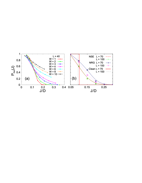
Figure 4: (Color online) Fraction of free moments as function of exchange coupling obtained by two methods: (a) From the condition that the NSE has no solution; (b) from temperature dependence of local spin susceptibility calculated with NRG for disorder $W=2$. The corresponding NSE result, and the fraction of free moments in a clean sample (step functions) are plotted for comparison. Lattice sizes are indicated. The lines are guides to the eye.

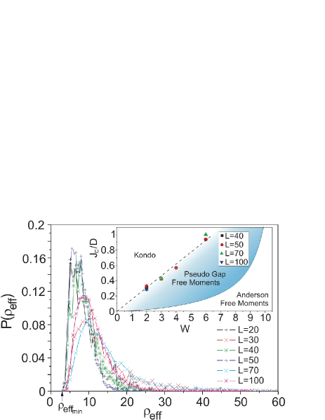
Figure 5: (Color online) The distribution of $\rho_{\rm eff}$ for $W=2$ and various lattice sizes. Inset: The magnetic impurity phase diagram in the $(J,W)$ plane. The data points correspond to $J_{\rm c}=1/\rho_{\rm eff_{min}}$ as function of $W$, obtained numerically for several system sizes. The straight line is a guide to the eye. The critical exchange coupling expected due to the hard gap caused by Anderson localization, $J_{\rm c}^{\rm A}$ [see Eq. (5)] is plotted for comparison (full line). For $J>J_{\rm c}$, all magnetic moments are screened (Kondo phase). For $J<J_{\rm c}^{\rm A}$, all magnetic moments remain free due to Anderson localization, the Anderson free moment phase. In the intermediate phase there is a finite probability that some magnetic moments remain unscreened due to the random occurence of local pseudo gaps.

Free Moment Phase. Next, we use NRG to analyze in detail the impurity sites where the renormalization of the magnetic susceptibility remains so small that no finite Kondo temperature can be defined. On such sites a magnetic moment remains free down to the lowest temperatures, the spin susceptibility $\chi_{\rm loc}$ diverges and $T\chi_{\rm loc}(T)$ approaches a finite value, as seen in Fig. 3b. We employed this criterion to identify free magnetic moments. In Fig. 4, we compare the resulting fraction of free moments with that derived from the condition that Eq. (3) has no finite $T_{K}$ solution. We see that the fraction of free moments obtained from NSE is smaller than the one from NRG. This can be attributed to the fact that higher-loop corrections tend to lower $T_{K}$. Thus, the criterion that the NSE has no solution gives a lower bound for the fraction of free magnetic moments. This criterion corresponds to setting $T_{K}\rightarrow 0$ in Eq. (3). Therefore, free moments exist when the effective, weighted LDOS as defined by,

$$\rho_{\rm eff}=\frac{1}{2N}\sum_{n=1}^{N}\frac{L^{2}|\psi_{n}({\bf r})|^{2}}{\mid E_{n}-E_{\rm F}\mid},$$ (4)

is equal or smaller than the inverse exchange coupling $1/J$. For a fixed realization of the disorder, this yields a lower bound for the critical exchange coupling $J_{\rm c}$ below which the magnetic impurity remains unscreened. For a clean system with a flat band, $\rho_{\rm eff}$ diverges logarithmically with the number of states $N$ or, equivalently, the volume. Then, $J_{\rm c}/D\sim 1/\ln N$. Since $T_{K}\sim D\exp(-D/J)$, the condition for free moments becomes $\Delta>c\,T_{K}$, with a constant $c\gg 1$ which depends on $E_{\rm F}$. In a clean system the level spacing vanishes in the thermodynamic limit, therefore there are no free moments for any finite $J$. Can one conclude the same when nonmagnetic disorder is present? No, for the following two reasons. First, let us note that for disordered systems with dimensions $d\leq 2$, all energy eigenstates are localized in the absence of spin-orbit interaction or a strong magnetic field. A finite local gap of order $\Delta_{\rm c}=1/(\nu\xi^{d})$ develops at the Fermi energy, where $\nu$ is the average density of states and $\xi$ is the average localization length. Therefore, there are with certainty free moments whenever $\Delta_{\rm c}\gg T_{K}$, or, equivalently, $J\ll J_{\rm c}^{\rm A}\sim D/\ln N_{\rm c}$, where $N_{\rm c}=D/\Delta_{\rm c}$. However, in weakly disordered two-dimensional electronic systems $\xi(g)=g\exp(\pi g)$ in the absence of an applied magnetic field. Here, the dimensionless disorder parameter $g=E_{\rm F}\tau$ is for quarter filling related to the disorder amplitude $W$ as $g=96/(\pi W^{2})$. Using Eq. (4) we then find

$$J_{\rm c}^{\rm A}=D\,\left[\ln\left(2\xi(W)^{2}\right)+C\right]^{-1},$$ (5)

where $C\approx 0.58$. This expression only provides a lower bound for $J_{\rm c}$ because both the localization length and the LDOS are widely distributed in a disordered system. In Fig. 5 we show the distribution of $\rho_{\rm eff}$ for moderate disorder and various lattice sizes. Remarkably, the point where the distribution drops sharply to zero, $\rho_{\rm eff_{min}}$, hardly depends on lattice size. In the inset of Fig. 5 we plot $J_{c}=1/\rho_{\rm eff_{min}}$ as a function of disorder for various system sizes, together with $J_{\rm c}^{\rm A}(W)$, Eq. (5). This plot shows a quantum phase diagram in the $(J,W)$ plane with a free magnetic moment phase due to Anderson localization for $J<J_{\rm c}^{\rm A}$ and a Kondo screened phase for $J>J_{c}(W)$. For intermediate couplings, $J_{\rm c}^{\rm A}<J<J_{c}(W)$, we also find free magnetic moments for all system sizes considered. It is well known that a free moment phase exists when there is a pseudogap around the Fermi energy gapless . Indeed, as seen in Fig. 3b, there is a dip in the LDOS at sites where the magnetic moment remains unscreened. In weakly disordered metals, the LDOS is correlated over a macroscopic energy interval of order of the elastic scattering rate $1/\tau$  mirlin . Although these correlations are only of order $1/g$ and the LDOS can fluctuate in energy, they can still cause dips in the LDOS within a range of order $1/\tau$. From the numerical results for $J_{c}(W)$ (inset of Fig. 5) we infer that the local pseudogaps in weakly disordered metals have a power that increases with disorder as $\alpha\sim W/D\sim 1/\sqrt{g}$.

The authors gratefully acknowledge useful discussions with Christopher Bäuerle, Harold Baranger, Ribhu Kaul, Ganpathy Murthy, Achim Rosch, Laurent Saminadayar, Denis Ullmo, and Gergely Zárand. S.K. and E.R.M. gratefully acknowledge the hospitalities of the Condensed Matter Theory Group at Boston University, the Max-Planck Institute for Physics of Complex Systems, and the Aspen Center for Physics. This research was supported by the German Research Council under SFB 668, B2, SFB 508, B9, and KE 807/2-1. A.Z. acknowledges support by the Grant No. 4640.2006.2 from the Russian Basic Research Foundation and by the Ural Division of RAS.

References

- (1) E. Miranda and V. Dobrosavljević, Rep. Prog. Phys. 68, 2337 (2005).
- (2) E. Miranda, V. Dobrosavljević, and G. Kotliar, J. Phys. Cond. Mat. 8, 9871 (1996).
- (3) R. N. Bhatt and D. S. Fisher, Phys. Rev. Lett. 68, 3072 (1992); A. Langenfeld and P. Wölfle, Ann. Physik 4, 43 (1995).
- (4) G. Zarand and L. Udvardi, Phys. Rev. B 54, 7606 (1996); S. Suga and T. Ohashi, J. Phys. Soc. Jpn. 72 Suppl. A, 139 (2003); R. K. Kaul, D. Ullmo, S. Chandrasekharan, and H. U. Baranger, Europhys. Lett. 71, 973 (2005); S. Chakravarty and C. Nayak, Int. J. Mod. Phys. B 14, 1421 (2000); G. Zaránd, L. Borda, J. von Delft, and N. Andrei, Phys. Rev. Lett. 93, 107204 (2004).
- (5) S. Kettemann and E. R. Mucciolo, JETP Lett. 83, 240 (2006) [Pis’ma v ZhETF 83, 284 (2006)]; S. Kettemann and E. R. Mucciolo, Phys. Rev. B 75, 184407 (2007).
- (6) T. Micklitz, A. Altland, T. A. Costi, and A. Rosch, Phys. Rev. Lett. 96, 226601 (2006).
- (7) S. Kettemann and M. E. Raikh, Phys. Rev. Lett. 90, 146601 (2003).
- (8) C. H. Lewenkopf and H. A. Weidenmüller, Phys. Rev. B 71, 121309(R) (2005).
- (9) J. Yoo, S. Chandrasekharan, R. K. Kaul, D. Ullmo, and H. U. Baranger, Phys. Rev. B 71 201309(R) (2005).
- (10) R. K. Kaul, D. Ullmo, and H. U. Baranger, Phys. Rev. B 68, 161305(R) (2003).
- (11) P. S. Cornaglia, D. R. Grempel, and C. A. Balseiro, Phys. Rev. Lett. 96, 117209 (2006).
- (12) T. Micklitz, T. A. Costi, and A. Rosch, Phys. Rev. B 75, 054406 (2007).
- (13) G. Bergmann, Phys. Rev. Lett. 58, 1236 (1987); R. P. Peters, G. Bergmann and R. M. Mueller ibid. 58, 1964 (1987); C. Van Haesendonck, J. Vranken, and Y. Bruynseraede, ibid. 58, 1968 (1987); J. J. Lin and N. Giordano, Phys. Rev. B 35, 1071 (1987); P. Mohanty and R. A. Webb, Phys. Rev. Lett. ibid. 84, 4481 (2000); F. Schopfer, C. Bäuerle, W. Rabaud, and L. Saminadayar, ibid. 90, 056801(2003); F. Mallet, J. Ericsson, D. Mailly, S. Unlubayir, D. Reuter, A. Melnikov, A.D. Wieck, T. Micklitz, A. Rosch, T. A. Costi, L. Saminadayar, and C. Bäuerle, ibid. 97, 226804 (2006); G. M. Alzoubi and N. O. Birge, ibid. 97, 226803 (2006).
- (14) O. O. Bernal, D. E. MacLaughlin, H. G. Lukefahr, and B. Andraka, Phys. Rev. Lett. 75, 2023 (1995).
- (15) D. Withoff and E. Fradkin, Phys. Rev. Lett. 64, 1835 (1990); K. Ingersent, Phys. Rev. B 54, 11936 (1996); L. Fritz, S. Florens, and M. Vojta, Phys. Rev. B 74, 144410 (2006).
- (16) J. K. Cullum and R. K. Willoughby, Lanczos algorithms for large symmetric eigenvalue problems (Birkhäuser, Boston, 1985); I. Kh. Zharekeshev and B. Kramer, Computer Phys. Commun. 121/122, 502 (1999).
- (17) Y. Nagaoka, Phys. Rev. 138, 1112 (1965); H. Suhl, Phys. Rev. A 138, 515 (1965).
- (18) K. G. Wilson, Rev. Mod. Phys. 47, 773 (1975).
- (19) H. R. Krishna-murthy, J. W. Wilkins, and K. G. Wilson, Phys. Rev. B 21, 1003 (1980); ibid. 21, 1044 (1980).
- (20) A. M. Clogston and P. W. Anderson, Bull. Am. Phys. Soc. 6, 124 (1961).
- (21) A. C. Hewson, The Kondo Problem to Heavy Fermions, Cambridge Univ. Press (1997).
- (22) G. E. Santoro and G. F. Giuliani, Phys. Rev. B 44, 2209 (1992).
- (23) A. N. Rubtsov and A. I. Lichtenstein, Pis’ma JETP 80, 67 (2004).
- (24) A. Zhuravlev, E. Gorelov, A. N. Rubtsov, S. Kettemann, and A. I. Lichtenstein, unpublished (2006).
- (25) M. T. Glossop and K. Ingersent, Phys. Rev. B. 75, 104410 (2007).
- (26) A. D. Mirlin, Phys. Rep. 326, 259 (2000).