Ruppeiner Geometry of RN Black Holes: Flat or Curved?

Abstract

In some recent studies aman1 ; aman2 ; aman3 , Aman et al. used the Ruppeiner scalar as a measure of underlying interactions of Reissner-Nordström black holes, indicating that it is a non-interacting statistical system for which classical thermodynamics could be used at any scale. Here, we show that if we use the complete set of thermodynamic variables, a non-flat state space will be produced. Furthermore, the Ruppeiner curvature diverges at extremal limits, as it would for other types of black holes.

I Introduction

It has been commonly held that black holes are thermodynamic systems davies ; wald . Black holes obey four laws of black hole mechanics analogous to the four laws of ordinary thermodynamics, posing a Bekenstein-Hawking entropy and a characteristic Hawking temperature related to the surface gravity of event horizon Bek ; BCH ; hawking1 ; hawking2 . Finding the underlying microscopic description of this entropy is one of the most challenging subjects in theoretical physics, but it still remains obscure, best left for future development of quantum theory of gravity jacobson .

Thermodynamic fluctuation theory, whose basic goal is to express the time independent probability distribution for the state of a fluctuating system in terms of thermodynamic quantities, is usually attributed to Einstein who applied it to the problem of blackbody radiation einstein . However, despite a wide range of applications, the classical fluctuation theory fails near critical points and for volumes in the order of the correlation volume or less. In 1979, Ruppeiner ruppeiner1 introduced a Riemannian metric structure representing thermodynamic fluctuation theory, and related it to the second derivatives of the entropy. His theory offered a good meaning for the distance between thermodynamic states. He showed that the breakdown of the classical theory was due to its failure to take account of local correlations ruppeiner2 . One of the most significant topics of this theory is the introduction of the Riemannian thermodynamic curvature as a qualitatively new tool for the study of fluctuation phenomena. This curvature has a possible relationship with the interactions of the underlying statistical system as proposed by Ruppeiner ruppeiner3 in contrast with single-component ideal gas which is a non-interacting system with zero Ruppeiner curvature. Earlier, in 1975, Weinhold weinhold had proposed an approach which was based on a sort of Riemanian metric defined as the Hessian of the internal energy of a given system, $M$, where derivatives are taken with respect to the extensive thermodynamic variables and entropy. In 1984, Mrugała mrugala and Salamon et al. salamon proved that these two metrics are conformally equivalent with the inverse of the temperature, $\beta$, as the conformal factor

$$ds^{2}_{R}=\beta ds^{2}_{W}$$ (1)

Since then, geometrical approaches have been intensively used to study the chemical and physical properties of various thermodynamic systems ruppeiner3 , first applied to black holes by Ferrara et al. ferrara to discuss the critical behavior in moduli space. Later, some authors used Ruppinier geometry to study phase space, critical behavior, and stability of various types of black hole families aman1 ; aman2 ; aman3 ; cai1 ; cai2 ; sarkar .

Recently, in a series of papers aman1 ; aman2 ; aman3 , Aman et al. derived Ruppeiner and Weinhold scalars for Reissner-Nordström (RN), Kerr, and BTZ black holes in arbitrary four dimensional space times. One of their results is that the Ruppeiner curvature is zero for RN black holes of any dimensions; however, for RN-AdS and Kerr black holes thermodynamic spaces are non-trivial and curvatures diverge at extremal limits aman1 . On the other hand, it seems that a non-interacting background can not produce the thermodynamic behavior of the RN black holes, so efforts were made to redefine Ruppeiner geometry using new Massiue functions cai2 . Furthermore, if one uses the Ruppeiner curvature, as proposed in ruppeiner3 , to find a lower volume as the limit of the applicability of classical thermodynamics, zero curvature will tell us that there is no such limit. This seems unacceptable because we expect classical description to fail at least at the Planck scale.

In this paper, we propose that a better measure of microscopic interactions will be obtained if one uses the complete phase space of extensive variables. According to this view, in calculating Ruppeiner curvature for RN black holes, one should set $J\rightarrow 0,l\rightarrow\infty$ limits in the scalar curvature of the Kerr-Newmann-AdS (KN-AdS) black hole, which is the most general solution of Einstein-Maxwell field equations in an anti-de Sitter background. The Ruppeiner curvature becomes a non-zero function of $M$ and $Q$ and diverges at extremal limits. This also indicates that classical thermodynamics could not be used for black holes of the size of Planck length. We believe that this is a general property which is related to the nature of fluctuation theory and is applicable for BTZ black holes that also have a flat Ruppeiner curvature in Aman’s method aman1 . Furthermore, using the quasilocal thermodynamic parameters shows that our results do not contingent upon using of ADM parameters.

The structure of the paper is as follows: In section II, we recall the charged rotating solution of the Einstein-Maxwell-anti-deSitter equations. We also recall the results of generalized Smarr formula for this type of black holes and derive the Ruppeiner curvature. In section III and IV, we discuss the ideas for the RN and Kerr families and discuss the phase transition points and their thermodynamic stability. In section V, we study the Ruppeiner geometry of KN and RN black holes by using the quasilocal thermodynamic quantities. Throughout this paper, we use the natural units $c=G=\hbar=1$ and also set $k_{B}=\frac{1}{\pi}$.

II Kerr-Newmann-AdS black holes

Here we consider the usual charged rotating black hole in AdS space. Its metric, which is axisymmetric, reads in Boyer-Lidquist type coordinates

$$ds^{2}=-{\Delta_{r}\over\rho^{2}}\left[dt-\frac{a\sin^{2}\theta}{\Xi}\ d\phi\right]^{2}+{\rho^{2}\over\Delta_{r}}\ dr^{2}+{\rho^{2}\over\Delta_{\theta}}\ d\theta^{2}+{\Delta_{\theta}\sin^{2}\theta\over\rho^{2}}\left[a\ dt-\frac{r^{2}+a^{2}}{\Xi}\ d\phi\right]^{2}$$ (2)

where

$$\rho^{2}=r^{2}+a^{2}\cos^{2}\theta,\qquad\Xi=1-{a^{2}\over l^{2}}$$ (3)

$$\Delta_{r}=(r^{2}+a^{2})(1+{r^{2}\over l^{2}})-2mr+q^{2},\qquad\Delta_{\theta}=1-{a^{2}\over l^{2}}\cos^{2}\theta$$ (4)

Here $a$ denotes the rotational parameter, $q$ is the electric charge, and $l$ is defined by $l^{2}=\frac{-3}{\Lambda}$, where $\Lambda$ is the cosmological constant. The mass $M$, charge $Q$ and the angular momentum $J$ can be defined by means of Komar integrals as

$$M=\frac{m}{\Xi^{2}},\qquad Q=\frac{q}{\Xi},\qquad J=\frac{am}{\Xi^{2}}$$ (5)

From these relations, one can obtain a generalized Smarr formula for Kerr-Newmann-AdS black holes, which reads caldarelli

$$\begin{split}M=\sqrt{\frac{S}{4\pi}+\frac{\pi}{4S}(4J^{2}+Q^{4})+\frac{Q^{2}}{2}+\frac{J^{2}}{l^{2}}+\frac{S}{2\pi l^{2}}\left(Q^{2}+\frac{S}{\pi}+\frac{S^{2}}{2\pi^{2}l^{2}}\right)}.\end{split}$$ (6)

$(S$, $J$, $Q)$ and (6) will be regarded as the complete set of energetic extensive parameters and the black hole thermodynamic fundamental relation, $M=M(S,Q,J).$ Conjugate variables to $S$, $Q$ and $J$ could be obtained, for example, the Hawking temperature is defined as : $T=\frac{\partial M}{\partial S}|_{\tiny{JQ}}$. Extremal black holes have a zero Hawking temperature; so, $T(S,Q,J)=0$ is used to calculate the extremal surface: $J=J_{extr}(S,Q)$. Now, components of the Ruppeiner metric could be derived

$$g_{ij}=\frac{1}{T}\frac{\partial^{2}M}{\partial X^{i}\partial X^{j}}\qquad X^{i}=(S,Q,J)$$ (7)

$$g_{11} = \frac{1}{2S(9S^{2}+36J^{2}+9Q^{4}+18Q^{2}S-12J^{2}\Lambda S-6S^{2}\Lambda Q^{2}-6S^{3}\Lambda+S^{4}\Lambda^{2})}$$ (8)

$$\times \frac{1}{\left(3{S}^{2}-12{J}^{2}-3{Q}^{4}-2{S}^{2}\Lambda{Q}^{2}-4{S}^{3}\Lambda+{S}^{4}{\Lambda}^{2}\right)}\times\bigl{(}-27{S}^{4}-432{J}^{2}{S}^{2}\Lambda{Q}^{2}$$

$$- 108{S}^{4}\Lambda{Q}^{2}-864{J}^{2}{S}^{3}\Lambda+360{J}^{2}{S}^{4}{\Lambda}^{2}+1296{J}^{4}+81{Q}^{8}+648{S}^{2}{J}^{2}$$

$$+ 162{S}^{2}{Q}^{4}+18{S}^{6}{\Lambda}^{2}+648{J}^{2}{Q}^{4}-8{S}^{7}{\Lambda}^{3}+{S}^{8}{\Lambda}^{4}-108{Q}^{6}{S}^{2}\Lambda$$

$$- 216{Q}^{4}{S}^{3}\Lambda+54{Q}^{4}{S}^{4}{\Lambda}^{2}+72{S}^{5}{\Lambda}^{2}{Q}^{2}-12{S}^{6}{\Lambda}^{3}{Q}^{2}-144{Q}^{4}{J}^{2}\Lambda S$$

$$+ 216{Q}^{6}S+864{J}^{2}{Q}^{2}S-576{J}^{4}\Lambda S-48{S}^{5}{\Lambda}^{3}{J}^{2}\bigr{)}$$

$$g_{12}=g_{21} = \frac{2Q}{\left(9{S}^{2}+36{J}^{2}+9{Q}^{4}+18{Q}^{2}S-12{J}^{2}\Lambda S-6{S}^{2}\Lambda{Q}^{2}-6{S}^{3}\Lambda+{S}^{4}{\Lambda}^{2}\right)}$$ (9)

$$\times \frac{1}{\left(3{S}^{2}-12{J}^{2}-3{Q}^{4}-2{S}^{2}\Lambda{Q}^{2}-4{S}^{3}\Lambda+{S}^{4}{\Lambda}^{2}\right)}\times\bigl{(}-27{S}^{3}+{S}^{6}{\Lambda}^{3}$$

$$+ 108S{J}^{2}-81{Q}^{2}{S}^{2}+54{Q}^{2}{S}^{3}\Lambda-9{Q}^{2}{S}^{4}{\Lambda}^{2}-108{J}^{2}{Q}^{2}-27{Q}^{6}$$

$$- 108{J}^{2}{S}^{2}\Lambda+27{Q}^{4}{S}^{2}\Lambda+27{S}^{4}\Lambda-81{Q}^{4}S-9{S}^{5}{\Lambda}^{2}$$

$$+ 72{Q}^{2}{J}^{2}\Lambda S+24{S}^{3}{\Lambda}^{2}{J}^{2}\bigr{)}$$

$$g_{13}=g_{31} = \frac{12J}{\left(9{S}^{2}+36{J}^{2}+9{Q}^{4}+18{Q}^{2}S-12{J}^{2}\Lambda S-6{S}^{2}\Lambda{Q}^{2}-6{S}^{3}\Lambda+{S}^{4}{\Lambda}^{2}\right)}$$ (10)

$$\times \frac{1}{\bigl{(}3{S}^{2}-12{J}^{2}-3{Q}^{4}-2{S}^{2}\Lambda{Q}^{2}-4{S}^{3}\Lambda+{S}^{4}{\Lambda}^{2}\bigr{)}}\times\bigl{(}-27{S}^{2}+27{S}^{3}\Lambda$$

$$- 36{J}^{2}+12{J}^{2}\Lambda S-9{Q}^{4}-3{Q}^{4}S\Lambda+18{S}^{2}\Lambda{Q}^{2}-2{S}^{3}{\Lambda}^{2}{Q}^{2}-9{S}^{4}{\Lambda}^{2}$$

$$+ {S}^{5}{\Lambda}^{3}-36{Q}^{2}S\bigr{)}$$

$$g_{22} = -\frac{4S}{\left(9{S}^{2}+36{J}^{2}+9{Q}^{4}+18{Q}^{2}S-12{J}^{2}\Lambda S-6{S}^{2}\Lambda{Q}^{2}-6{S}^{3}\Lambda+{S}^{4}{\Lambda}^{2}\right)}$$ (11)

$$\times \frac{1}{\left(3\,{S}^{2}-12\,{J}^{2}-3\,{Q}^{4}-2\,{S}^{2}\Lambda\,{Q}^{2}-4\,{S}^{3}\Lambda+{S}^{4}{\Lambda}^{2}\right)}\times\bigl{(}-27{S}^{3}+{S}^{6}{\Lambda}^{3}$$

$$- 108S{J}^{2}-81{Q}^{2}{S}^{2}+54{Q}^{2}{S}^{3}\Lambda-9{Q}^{2}{S}^{4}{\Lambda}^{2}-324{J}^{2}{Q}^{2}-27{Q}^{6}$$

$$+ 72{J}^{2}{S}^{2}\Lambda+27{Q}^{4}{S}^{2}\Lambda+27{S}^{4}\Lambda-81{Q}^{4}S-9{S}^{5}{\Lambda}^{2}$$

$$+ 108{Q}^{2}{J}^{2}\Lambda S-12\,{S}^{3}{\Lambda}^{2}{J}^{2}\bigr{)}$$

$$g_{23}=g_{32} = -\,{\frac{48SQJ\left(-3\,{Q}^{2}-3\,S+{S}^{2}\Lambda\right)\left(-3+S\Lambda\right)}{\left(9\,{S}^{2}+36\,{J}^{2}+9\,{Q}^{4}+18\,{Q}^{2}S-12\,{J}^{2}\Lambda\,S-6\,{S}^{2}\Lambda\,{Q}^{2}-6\,{S}^{3}\Lambda+{S}^{4}{\Lambda}^{2}\right)}}$$ (12)

$$\times \frac{1}{\left(3\,{S}^{2}-12\,{J}^{2}-3\,{Q}^{4}-2\,{S}^{2}\Lambda\,{Q}^{2}-4\,{S}^{3}\Lambda+{S}^{4}{\Lambda}^{2}\right)}$$

$$g_{33} = -{\frac{8S\left(9\,{S}^{2}-6\,{S}^{2}\Lambda\,{Q}^{2}+9\,{Q}^{4}+18\,{Q}^{2}S-6\,{S}^{3}\Lambda+{S}^{4}{\Lambda}^{2}\right)\left(-3+S\Lambda\right)}{\left(9\,{S}^{2}+36\,{J}^{2}+9\,{Q}^{4}+18\,{Q}^{2}S-12\,{J}^{2}\Lambda\,S-6\,{S}^{2}\Lambda\,{Q}^{2}-6\,{S}^{3}\Lambda+{S}^{4}{\Lambda}^{2}\right)}}$$ (13)

$$\times \frac{1}{\left(3\,{S}^{2}-12\,{J}^{2}-3\,{Q}^{4}-2\,{S}^{2}\Lambda\,{Q}^{2}-4\,{S}^{3}\Lambda+{S}^{4}{\Lambda}^{2}\right)}$$

Furthermore, by definition of the Ricci scalar carroll , the Ruppeiner curvature could be calculated directly by using GRTensor II or GRTensor M packages. The expression is too complicated to present here, so the results are depicted numerically. The Ruppeiner curvature diverges at the extremal limit, $J_{1}=J_{extr}(S,Q)$, and along the surface $J_{2}(S,Q)$ where metric changes its sign (a signature of thermal instability). For different combinations of $S$ and $Q$, each $J$ function has a double root, so at four physically acceptable values of $J$, the scalar curvature diverges. The Ruppeiner geometry is not flat (Fig. 1), a fact that could also be checked by the Cotton-York tensor.

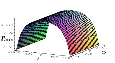
Figure 1: Ruppeiner curvature of KN-AdS BHs as a function of $Q$ and $J$. We set $S=100$ and $\Lambda=-1$. The plot shows the region between the first two divergent points, which indicates that it is a non-flat Ruppeiner curvature.

III RN black holes, the matter of statistical interactions?

Up untill now, we have been considering the RN case which is our main interest, because of the works by Aman et al. aman1 ; aman2 ; aman3 , indicating that this family of black holes has a trivial thermodynamic geometry (zero curvature) and so has a non-interacting underlying statistical system. This can be an interesting result which may serve as a guide in looking for an appropriate statistical model for black holes in loop quantum gravity or string theory. On the other hand, it seems that the physical structure of RN black holes could not be reproduced by such a simple underlying system. Furthermore, the absence of the divergent points set it in a different class from other types of black holes. If RN systems are viewed as the limit of KN-AdS black holes by setting $l\rightarrow\infty$ and $J\rightarrow 0$ in the Ruppeiner curvature calculated for KN-AdS case, $R$ will takes the form

$$R=\frac{S^{2}+Q^{2}S+2Q^{4}}{(S^{2}-Q^{4})(S+Q^{2})}$$ (14)

We now have a new non-zero Ruppeiner scalar which diverges at the extremal limits: $Q=\pm\sqrt{S}$ (Fig. 2). This observation is in agreement with pavon , which used the second moments of the fluctuations in the fluxes of energy and angular momentum. It was shown that phase transitions occur only at the extremal limits, the points at which a black hole changes its nature to a naked singularity, a new phase.

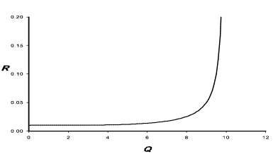
Figure 2: Ruppeiner scalar of RN BH ($l\rightarrow\infty,J\rightarrow 0$) as a function of $Q$. $R$ diverges at $Q=\pm 10$. Even at $Q=0$, $R$ has a $\frac{1}{S}$ remnant.

It should be noted that this behavior is related to the nature of the Ruppeiner geometry. If we initially work with spinless black holes

$$g_{ij} = \frac{1}{T}\frac{\partial^{2}M}{\partial X^{i}\partial X^{j}}\qquad X^{i}=(S,Q)$$

$$g_{11}=\frac{3Q^{2}-S}{2S(S-Q^{2})},\qquad g_{21} =g_{12}=-\frac{2Q}{S-Q^{2}},\qquad g_{22}=\frac{4S}{S-Q^{2}}$$ (15)

we will neglect the fluctuations of parameter $J$ in all calculations, which will lead to a wrong flat geometry ($R=0$). Therefore, the above non-vanishing scalar curvature is a result coming from another dimension specified by $J$ which fluctuates even if we set it to zero. We see that by setting $J=\Lambda=0$, the metric elements of KN-AdS state space (Eqs. 7-13) reduce to the RN ones (Eq. 15) but the curvature does not behave in the same manner. This behavior originated from the existence of an extra dimension in the parameter space. When the extremal limit is approached, however, the curvature diverges strongly. Another difference is also observed from reports in certain works on RN black holes phase space: the absence of ’Davies phase transition points’. This relates to the difference between ordinary thermodynamics of extensive systems and that of black holes, which constitute non-extensive, non-additive thermodynamic systems because of the well known scaling of the black hole entropy with area rather than with volume. However, the interpretation of the divergence in specific heats as phase transitions is not settled and has been the subject of much debate curir ; pavon ; kaburaki1 ; kaburaki2 ; sorkin . Ruppeiner formalism relies on the usual thermodynamic properties of extensive systems but it can also be applied to black holes near the divergent points arcioni . So we can use the Ruppeiner method as a probe to find phase transitions. Furthermore, Ruppeiner proposed that $\left|R\right|$ sets the limiting lower volume in which the classical fluctuation theory provides a good approximation ruppeiner3 . For black holes, it could be obtained from (7) that even for a non-charged black hole, Ruppeiner curvature has a $\frac{1}{S}$ remanent. Replacing $S$ by $\frac{s}{k_{B}}$, where $s$ is the entropy per volume, and leaving the choice of natural units, one could derive a lower volume, $v\simeq\frac{G\hbar r}{c^{3}}$ (in which $r$ is the Schwarzchild radius), above which the classical thermodynamic regime could be used. This also indicates that if the Schwarzchild radius of the black hole reaches the Planck length, $l_{p}=\sqrt{\frac{G\hbar}{c^{3}}}$, the classical thermodynamic description will break down.

Still another problem is that of stability. In order to determine the points where a change of thermodynamic stability occurs, we use Poincaré turning point method. According to Arcioni and Lozano-Tellechea arcioni , by plotting the conjugate variables ($\beta=\frac{1}{T},\frac{\phi}{T}=\frac{1}{T}\frac{\partial M}{\partial Q}$) in according to their extensive parameters ($M,Q$) one could see the points where black hole changes its stability (Figs. 3a & 3b). There is no turning point and, therefore, no changes of stability are shown along the plot. The first diagram shows that $\beta$ has a minimum at $M=\frac{2}{\sqrt{3}}$ (by setting $Q=1$). As described in arcioni , this is not a measure of changing stability, so nothing special happens at this point (Davies point).

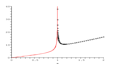
Figure 3: a) Dotted line - $\beta$ as a function of $x(=M)$ at fixed $Q$ ($Q=1$). $M\rightarrow\infty$ is the Schwarzchild limit, $M=1$ is the extremal limit and the plot has a minimum at $M=\frac{2}{\sqrt{3}}$ (Davies point) but there is no turning point.
b) Line -$\frac{\phi}{T}$ as a function of $x(=Q)$ at fixed $M$ ($M=1$). $Q\rightarrow 0$ is the Schwarzchild limit and $Q=1$ is the extremal limit.

IV Kerr black holes

Aman et al. also calculated the Ruppeiner and Weinhold’s curvatures for rotating black holes against a flat background. They reported a vanishing Weinhold curvature for Kerr-type black holes but also noted that the physical meaning of this property was not clear which they referred to as the ad hoc definition of Weinhold geometry aman1 ; aman2 . Using the definition of Weinhold’s metric weinhold for the complete phase space of parameters (KN-AdS black hole), and taking the limits $Q\rightarrow 0$, $l\rightarrow\infty$, a non vanishing Weinhold curvature is derived. The phase transition points could be obtained by calculating the Ruppeiner curvature

$$R_{kerr}=\frac{S(S^{2}+36J^{2})}{S^{4}-16J^{4}}$$ (16)

$R_{kerr}$ diverges at the extremal limits: $J=\pm\frac{S}{2}$ (Fig. 4). Further, one could easily check the instabilities by using the Poincaré diagrams: $(\beta(M),M)$ and $(\frac{\omega(J)}{T},J)$. The plots do not show any turning points (and thus no instability) as indicated before in kaburaki1 ; kaburaki2 ; arcioni .

V Geometry of Quasilocal Thermodynamics

In this section we replace our definition of the internal energy of black holes by quasilocal energy proposed by Brown and York brown1 ; brown2 which is derived from the Hamiltonian of spatially bounded gravitational systems.

The Brown-York derivation of the quasilocal energy, as applied to a four-dimensional (4D) spacetime solution of Einstein gravity can be summarized as follows. The system one considers is a 3D spatial hypersurface $\Sigma$ bounded by a 2D spatial surface $B$ in a spacetime region that can be decomposed as a product of a 3D hypersurface and a real

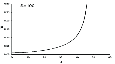
Figure 4: Ruppeiner scalar of Kerr BH as a function of $J$. $R$ diverges at two values of $J$. Even at $J=0$, $R$ has a $\frac{1}{S}$ remnant.

line-interval representing time. The time-evolution of the boundary $B$ is the surface ${}^{3}B$. One can then obtain a surface stress-tensor on ${}^{3}B$ by taking the functional derivative of the action with respect to the 3D metric on ${}^{3}B$. The energy surface density is the projection of the surface stress-tensor normal to a family of spacelike surfaces such as $B$ that foliate ${}^{3}B$. The integral of the energy surface density over such a boundary $B$ is the quasilocal energy associated with a spacelike hypersurface $S$ whose orthogonal intersection with ${}^{3}B$ is the boundary $B$. It is assumed that there are no inner boundaries, such that the spatial hypersurfaces $S$ are complete. In the case where horizons form, one simply evolves the spacetime inside as well as outside the horizon. Under these conditions, the QLE (Quasi Local Energy) is defined as:

$$E=\frac{1}{8\pi}\oint_{B}d^{2}x\sqrt{\sigma(k-k_{0})}$$ (17)

where $\sigma$ is the determinant of the 2-metric on $B$, $k$ is the trace of the extrinsic curvature of $B$, and $k_{0}$ is a reference term that is used to normalize the energy with respect to a reference spacetime, not necessarily flat. To compute the QLE for asymptotically flat solutions, one can choose the reference spacetime to be flat as well. In that case, $k_{0}$ is the trace of the extrinsic curvature of a two-dimensional surface embedded in flat spacetime, such that it is isometric to $B$.

For spacetimes that are asymptotically flat in spacelike directions, the quasilocal energy and angular momentum defined there agree with the results of Arnowitt, Deser and Misner in the limit that the boundary tends to spatial infinity adm ; martinez ; bose . We have used ADM parameters in the above discussions. Now, ADM mass ($M$) is replaced by quasilocal energy of KN black holes

$$E=r_{0}[1-\sqrt{1-\frac{2M}{r_{0}}+\frac{a^{2}+Q^{2}}{r_{0}^{2}}}]+O(\frac{a^{2}}{r_{0}})$$ (18)

where $a=\frac{J}{M}$ and $r_{0}$ is the radius of the bounding surface. Here we only consider the small electrical charge and slow rotating regime $(\frac{|a|}{r_{0}}\ll 1),$ so the definition of $Q$ and $J$ do not have to change. Inserting

$$M=\sqrt{\frac{S}{4}+\frac{1}{S}(J^{2}+\frac{Q^{4}}{4})+\frac{Q^{2}}{2}}$$ (19)

in (18) one could derive a new fundamental equation for quasilocal parameters

$$E(S,Q,J)=r_{0}\bigl{[}1-\sqrt{1-\frac{2\sqrt{\frac{S}{4}+\frac{1}{S}(J^{2}+\frac{Q^{4}}{4})+\frac{Q^{2}}{2}}}{r_{0}}+\frac{a^{2}+Q^{2}}{r_{0}^{2}}}\bigr{]}+O(\frac{a^{2}}{r_{0}})$$ (20)

Now the Ruppeiner metric components could be calculated

$$g_{ij}=\frac{1}{T}\frac{\partial^{2}E}{\partial X^{i}\partial X^{j}}\qquad X^{i}=(S,Q,J)$$ (21)

For RN black holes (2-dimensional state space) curvature is a function of $r_{0}$, such that

$$\lim_{r_{0}\rightarrow\infty}R_{RN}(r_{0},S,Q)=0$$ (22)

For Kerr-Newmann black holes (full thermodynamic state space) the calculated curvature is different from $R_{RN}$ for any finite value of $r_{0}$ (they are too large to be written here) and has the following limiting form:

$$\lim_{r_{0}\rightarrow\infty,J\rightarrow 0}R_{KN}(r_{0},S,Q,J)=\frac{S^{2}+Q^{2}S+2Q^{4}}{(S^{2}-Q^{4})(S+Q^{2})}$$ (23)

As expected this limit equals to (14). The above considerations show that our results do not contingent upon computing all thermodynamic quantities at infinity.

VI Conclusion

Usual statistical mechanics, augmented by renormalization group theory, are used to build up from the microscopic physics and deduce information about the macroscopic world. For the black holes, the microscopic description needs a quantum theory of gravity which is still missing. In contrast, the covariant thermodynamic fluctuation theory builds down from the macroscopic equation of states using the Riemannian geometry ruppeiner3 . In using this method one must be careful to consider all possible physical fluctuations because neglecting one parameter may lead to inadequate information about the model. For the RN case, the Ruppeiner curvature could be obtained using the complete set of physical fluctuating parameters. The resulting Ruppeiner curvature is not zero, behaves like other types of black holes, and could be used to set a lower bound, $R_{Sch}\simeq l_{p}$, beyond which the classical thermodynamic description breaks down as expected. The Method proposed here could also be applied to other cases, e.g., as shown by Henneaux and Teitelboim henax , it is possible to promote the cosmological constant to a thermodynamic state variable which may be the subject of future study.

References

- (1) J. E. Åman, I. Bengtsson and N. Pidokrajt, Gen. Rel. Grav. 35, 1733. (2003) [gr-qc/0304015]
- (2) J. E. Åman and N. Pidokrajt, Phys. Rev. D 73, 024017. (2006) [hep-th/0510139]
- (3) J. E. Åman and N. Pidokrajt, Gen. Rel. Grav. 38, 1305. (2006) [gr-qc/0601119]
- (4) P. C. W. Davies, Proc. Roy. Soc. Lon. A 353, 499 (1977)
- (5) R. M. Wald, Living Rev. Rel. 4, 6. (2001) [gr-qc/9912119]
- (6) J. D. Bekenstein, Phys. Rev. D 7, 2333. (1973)
- (7) J. M. Bardeen, B. Carter and S. W. Hawking, Commun. Math. Phys. 31, 161. (1973)
- (8) S. W. Hawking, Commun. Math. Phys. 43, 199. (1975)
- (9) S. W. Hawking, Nature 248, 30. (1974)
- (10) T. Jacobson, D. Marolf and C. Rovelli, Int. J. Theor. Phys. 44, 1807. (2005) [hep-th/0501103]
- (11) A. Einstein, Ann. Phys. (IV Folge) 22, 569 (1907)
- (12) G. Ruppeiner, Phys. Rev. A 20, 1608 (1979)
- (13) G. Ruppeiner, Phys. Rev. Lett. 50, 287 (1983)
- (14) G. Ruppeiner, Rev. Mod. Phys. 67, 605 (1995)
- (15) F. Weinhold, J. Chem. Phys. 63, 2479 (1975)
- (16) R. Mrugała, Physica A 125, 631 (1984)
- (17) P. Salamon, J. D. Nulton and E. Ihrig, J. Chem. Phys. 80, 436 (1984)
- (18) S. Ferrara, G. W. Gibbons and R. Kallosh, Nucl. Phys. B 500, 75 (1997) [hep-th/9702103]
- (19) R. G. Cai and J. H. Cho, Phys. Rev. D 60, 067502. (1999) [hep-th/9803261]
- (20) J. Shen, R. G. Cai, B. Wang and R. K. Su, [gr-qc/0512035].
- (21) T. Sarkar, G. Sengupta and B. N. Tiwari, JHEP 0611 (2006) 015, [hep-th/0606084].
- (22) M. M. Caldarelli G. Cognola and D. Klemm, Class.Quant.Grav. 17, 399. (2000) [hep-th/9908022]
- (23) S. Carroll, Spacetime and Geometry: An Introduction to General Relativity, Benjamin Cummings, 1st edition (2003).
- (24) A. Curir, Gen. Rel. Grav. 13, 417. (1981)
- (25) D. Pavón, Phys. Rev. D 43, 2495. (1991)
- (26) J. Katz, I. Okamoto and O. Kaburaki, Glass. Quant. Grav. 10, 1323. (1993)
- (27) O. Kaburaki, I. Okamoto and J. Katz, Phys. Rev. D 47, 2234. (1993)
- (28) R. D. Sorkin, Astrophys. J. 257, 847. (1982)
- (29) G. Arcioni and E. Lozano-Tellechea, Phys. Rev. D 72, 104021. (2005) [hep-th/0412118]
- (30) J. D. Brown and J. W. York, Jr., Phys. Rev. D 47, 1407 (1993).
- (31) J. D. Brown, J. Creighton and R. B. Mann, Phys. Rev. D 50, 6394 (1994).
- (32) R. Arnowitt, S. Deser, and C. W. Misner, in Gravitation: An Introduction to Current Research, edited by L. Witten, Wiley, New York, (1962).
- (33) E. A. Martinez, Phys. Rev. D 50, 4920 (1994).
- (34) S. Bose, T. Z. Naing, Phys. Rev. D 60, 104027 (1994).
- (35) M. Henneaux and C. Teitelboim, Commun. Math. Phys. 98, 391. (1985)